Improving the SPES protocol by automating ER and DR detection and evaluation of the spatial relation between ERs and DRs

(1)

U

niversity of

T

wente

M

aster

T

hesis

T

echnical

M

edicine

Improving the SPES protocol by automating ER

and DR detection and evaluation of the spatial

relation between ERs and DRs

Dorien van Blooijs

Graduation committee:

Chairman: prof. dr. ir. M.J.A.M. van Putten Technical supervisor: dr. H.G.E Meijer

Medical supervisor: dr. F.S.S. Leijten Process supervisor: dr. M. Groenier Extra member: dr. G.J.M. Huiskamp

(2)

(3)

Abstract

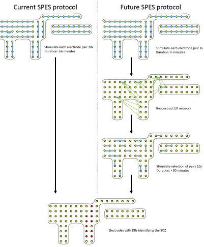
Introduction Epilepsy is one of the main causes of brain health disability. In 70% of the patients, seizure freedom is provided with medication. Patients with focal epilepsy, who have not responded to intensive medical treatment, are screened for the possibility of epilepsy surgery. When a visible lesion on an MRI image is found, and the lesion does not overlap with a functional area, the patient undergoes epilepsy surgery with acute electrocorticograpy (ECoG). In more complicated situations, when no visible lesion on an MRI image is found, or the lesion overlaps with functional areas, ECoG is performed with chronic grid implantation for maximally ten days. During this long-term ECoG recording, the seizure onset zone (SOZ) is delineated based on the seizures occurring during the chronic ECoG monitoring, and the resection area is determined based on the SOZ. The urge of having to have a seizure can be very stressful for the patient, and risks for complications are increased when chronic ECoG monitoring takes longer. Therefore, methods are investigated to delineate the SOZ faster and which are not based on seizures. In the future, such methods might replace chronic grid implantations by being performed during surgery to delineate both functional and resection areas.

With Single Pulse Electrical Stimulation (SPES), ten short electrical pulses are applied to stimulus pairs, which are neighboring electrodes on the electrode grid. SPES evokes early responses (ERs) and delayed responses (DRs). ERs are characterized as spikes or slow waves, starting within 100 ms after the stimulation artifact. ERs are proposed to reflect the physiological network. DRs are characterized as spikes or sharp waves occurring between 100 ms and 1 s after the stimulation artifact. DRs are proposed to be pathogenic and to correlate with the SOZ. Currently, the duration of the SPES protocol is at least one hour and the duration of visual analysis of the ERs and DRs takes almost one day. As a consequence, both the duration of SPES itself and the analysis are too long for usage during surgery. In this study, we have developed an automatic detection algorithm for ERs and DRs. We have also investigated the spatial relation between ERs and DRs. When we can discard stimulus pairs which will not evoke any DRs based on the physiological network from ERs, we can make the SPES protocol more time efficient.

Method For both ERs and DRs, two detectors were developed and compared. The first detector was based on an amplitude threshold. The peak from a spike or wave was considered as ER or DR when the peak exceeded a specific amplitude threshold. In the second detector, the standard deviation (SD) was calculated to distinguish an ER or DR from continuous spontaneous activity. A peak was considered as ER or DR when the ratio between the amplitude of a detected peak and the SD exceeded a specified SD factor.

In the ER detector, several parameters were varied: the amplitude threshold or SD factor, the minimal

SD and sel, a parameter in the Matlab functionpeakfinder, which detected a peak when the peak was

higher than the rest of the signal. The amplitude threshold was the value a peak had to exceed to be considered as ER or DR. The SD factor was a value, which the ratio between a the amplitude of a peak and the SD had to exceed, to be considered as ER or DR. The minimal SD was important in signals with very little spontaneous activity. In signals with a low SD, small peaks were easily considered as ER or DR. To prevent detection of these small peaks, a minimal SD had to be set.

In the DR detector, several parameters were varied as well. These parameters were the amplitude threshold or SD factor, sel and the cut off frequency (fc). The fc was implemented to prevent detection of high amplitude slow waves which were part of the ER, but present in the time window where DRs occurred.

Detections were compared with visual annotation. Sensitivity, specificity, positive predictive value (PPV) and negative predictive value (NPV) were calculated and ROC curves were made. The setting of parameters with the best performance was used in validation of the detectors.

(4)

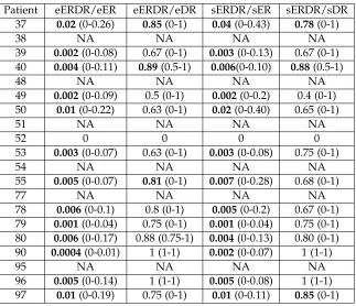
resulted in an ER or DR in this electrode were counted (sER/sDR). We distinguished the sERs and sDRs into stimulus pairs which only resulted in ERs or DRs (soER/soDR) or both ERs and DRs (sERDR). Per stimulus pair, the number of electrodes with an evoked ER or DR were counted (eER/eDR). We distinguished the groups of eERs and eDRs into electrodes in which only ERs or DRs were evoked

(eoER/eoDR) or both ERs and DRs were evoked (eERDR). We tested with a two sided t-test (α= 0.05)

whether the ratios of eERDR/eDR, eERDR/eER, sERDR/sER and sERDR/sDR differed significantly from 0.5. When ERs occurred equally in both signals with DRs and in signals without DRs, the ratio was 0.5. We tested whether ERs occurred significantly more often in signals with or without DRs. We also tested with a Mann Whitney U test whether more ERs were evoked in the electrodes in which DRs

were evoked, than in the electrodes in which no DRs were evoked (α=0.05). A similar analysis was used

for the stimulus pairs.

At last, we were allowed to execute a second SPES session. We investigated whether detected ERs are reproducible when the protocol is repeated, and we investigated the stimulation settings by comparing responses to pulses according to the standard SPES protocol and responses to pulses according to an alternative SPES protocol. In this alternative SPES protocol, we varied one parameter per situation. We varied the pulse form, the current intensity, and we applied a biphasic pulse instead of a monophasic pulse. To investigate reproducibility, we averaged the first three responses to an applied pulse per

electrode for each trial from the first SPES session in six patients (epoch13). We averaged the first three

responses to an applied pulse per electrode for each trial from the second SPES session in six patients

(epoch23). Bothepoch13andepoch23had the same settings (monophasic, positive pulse, 0.2 Hz, 8 mA,

1ms). We detected ERs in all averaged epochs13andepochs23. We calculated the total, positive and

negative agreement. When agreement was high, ERs are reproducible when the standard protocol is repeated.

To investigate whether neural stimulation is the greatest at the cathode, the anode or whether both electrodes contribute equal, we averaged the first three responses and the second three responses to

a pulse per electrode for each trial of the second SPES session in four patients (epochs23andepochs26

respectively). We used the automatic ER detector to detect ERs in both epochs23 andepochs26. To

investigate whether both electrodes contribute equally, we comparedepochs23andepochs26from the

same stimulus pair. epochs23 had a positive pulse form, epochs26 had a negative pulse form. To

investigate whether the anode contributed most, we comparedepochs23andepochs26from neighboring

electrodes in which one electrode is the anode. To investigate whether the cathode contributed most, we compared epochs from neighboring electrodes, in which one electrode is the cathode. We calculated the

total, positive and negative agreement for each situation. The Mann Whitney U test (α=0.05) was used

to determine whether one situation had a significantly better agreement than another test.

To investigate whether other ERs were evoked when a lower current intensity (4 mA) was used instead

of the standard current intensity (8 mA), we averaged epochs23 and epochs26 in four patients. We

detected ERs with the automatic detector in bothepochs23andepochs26. We calculated the total, positive

and negative agreement in each patients.

To investigate whether the same ERs are evoked when a biphasic pulse was applied instead of a

monophasic pulse, we averaged epochs23 and epochs26 in two patients. We detected ERs with the

automatic ER detector. We calculated the total, positive, and negative agreement in both patients.

Results The ER detector based on SD factor performed best with sensitivity, specificity, PPV and NPV

of respectively 0.78, 0.91, 0.75, 0.92 when SD factor = 2.5, sel = 20µV, minimal SD = 50µV.

The performance of the DR detector based on SD factor performed best with a sensitivity, specificity,

PPV and NPV of respectively 0.68, 0.92, 0.10 and 1.00 when SD factor = 4, minimal SD = 40µV, fc = 1

Hz.

(5)

that most ERs were evoked without a DR, but that most DRs are evoked with an ER. We found in one patient that in electrodes with evoked DRs, significantly more ERs were evoked. We found in six patients that stimulus pairs which resulted in DRs resulted in significantly more ERs.

When investigating the reproducibility of ERs, we found that the total, positive, negative agreement were respectively 0.85, 0.67, 0.90 on average in three out of six patients. The other three patients had a total, positive and negative agreement of respectively 0.67, 0.52, 0.75 on average. In the first three patients, the agreement is high. In the last three patients, the agreement is much lower. In the first three patients, the first SPES session was executed at least one day after surgery. In the last three patients, the first SPES session was executed on the same day as the grid implantation.

When investigating whether the anode, the cathode or both electrodes contribute equal to neural stimulation, we found a trend towards significance when we compared the total agreement and negative agreement between the situation in which both electrodes contribute equally and the situations in which the anode or cathode contributed more.

When investigating whether the same ERs are evoked with lower current intensity, we found that the total, positive and negative agreement between 4 and 8 mA were respectively 0.82, 0.52, 0.89 on average. When investigating whether a biphasic pulse evokes the same ERs, we found a total, positive and negative agreement of respectively 0.85, 0.63, 0.89 on average.

Conclusion The performance of the ER detector is sufficient for further usage in this study. The sensitivity and PPV of the DR detector are not very high since the number of annotated DRs is not very high. This means that a few false positive or false negative detections have a large effect on the sensitivity and the PPV. Due to the high number of false positive detections, the detected DRs were visually revised when we investigated the spatial relation between ERs and DRs.

We found that electrodes with DRs had more ERs and that stimulation pairs which evoked DRs evoked more ERs. This research is a first step in automatic detection of ERs and DRs and in gaining insight in the relation between ERs and DRs. In further research, it is recommended to investigate indirect connections in the network to gain more insight in the relation between ERs and DRs. The current ER and DR detector does not work well in detecting Stable Responses (SRs) and Repetitive Responses (RRs). Both detectors can be improved to enable detection of SRs and RRs.

When investigating the stimulus settings, we found a difference in reproducibility of ERs when the first SPES session was executed on the same day as the implantation surgery. These patients were still sleepy, and possibly anesthetics had some effect on the physiological networks in the brain.

(6)

(7)

Epilepsy is one of the main causes of brain health disability, especially among young adults, and accounts for a worldwide burden of illness similar to that of breast cancer in women and lung cancer in men [1, 2]. The incidence of epilepsy in the general population is approximately 45/100000 per year [3]; prevalence is 5.8 per 1000 [3] and the life-time probability of an epileptic seizure is approximately 3% [4]. In the Netherlands, there are approximately 84.000 patients with epilepsy [3].

Epilepsy is a disturbance in brain function, presenting itself with seizures with a variable frequency and duration [5]. Seizures are characterized by excessive or over-synchronized discharges of cerebral neurons [4]. Epilepsies are divided into two groups [6]: focal and generalized epilepsies [7, 8, 9]. The first group are epilepsies known variously as focal, partial or local [6]. Focal seizures arise from a focal or localized area of the brain [8] due to a tumor, ischemia, trauma, vascular malformation or other abnormalities of brain tissue [5], and the interictal EEG may show focal spikes and or sharp waves [7]. The second group contains epilepsies with seizures which arise from bilateral diffuse discharges in both hemispheres [8] and the EEG may show generalized, bilateral spike and wave discharges [7]. This group does not have an identifiable site of onset [6]. Generalized seizures involve deep structures such as the thalami to provide widespread synchronization. Both groups of epilepsies differ substantially in their pharmacology, cellular physiology and their clinical manifestations [6].

Medication is usually effective and provides seizure freedom in 70-80% of the patients [10]. Thus, about 20-30% of the patients with epilepsy have seizures that are not controlled by available anti-epileptic drugs [5, 11, 12]. When seizures persist after two consecutive years of medical treatment in which two or three first-line anti-epileptic drugs have failed, the odds are low (<5%) that they will ever be seizure free with drugs alone. Patients with focal epilepsy are then screened for epilepsy surgery [10, 11, 9, 3].

1.2 Surgery

The purpose of surgical treatment is to achieve seizure freedom in patients with intractable focal epilepsy that has a serious impact on their quality of life [5]. Results are good. With careful selection, only about 10% of patients obtain no improvement at all from epilepsy surgery and less than 5% worsen after surgery [8].

Using mainly non-invasive diagnostic techniques, the epilepsy focus is lateralized and localized at lobar or sublobar level. In the University Medical Center Utrecht (UMCU), most patients then undergo ’tailored’ epilepsy surgery with acute, i.e. intraoperative, electrocorticography (ECoG) in which signals from the brain are measured with electrode grids during surgery to precisely determine which area of brain tissue has to be resected.

(13)

[image:13.612.217.399.75.262.2]

Figure 1.1:This is a reconstruction of the brain in which an MRI scan is combined with a CT scan. This combination enables visualization of the location of the grid on the brain of a patient. This grid is placed for maximally ten days and records the brain signals.

1.3 Single Pulse Electrical Stimulation

The idea behind SPES is that the balance between excitability and inhibition of the brain is studied with brief single pulses. This activates only a limited and localized population of neurons instead of activating widespread cortex due to long trains of current pulses (1-5s) as has been previously used to induce habitual seizures [15, 16, 17]. During a SPES measurement in the UMCU, all neighboring electrode pairs on a grid, irrespective of particular placement of these electrodes across the gyri, are stimulated ten times [18]. The responses to these stimulations in other electrodes give information on the epileptogenicity of the tissue.

Valentin et al. saw two main types of responses: early responses and late responses [15, 16, 17]. An early response (ER) is characterized as a spike and/or slow wave starting within 100 ms after the stimulation artifact [15, 19]. It consists of a sharp deflection immediately following the stimulus artifact or occasionally merging with it [15, 16, 20]. This initial deflection is followed by one or two slow waves of alternating polarity [15]. These responses are seen in most regions in all patients and seem to be a normal response of the cortex to the stimulation [15, 16]. They may be viewed as cortico-cortical evoked potentials. ERs are recorded in areas around the stimulated cortex but sometimes also at a distance, providing evidence of functional connections between stimulated cortex and the regions where early responses are recorded [20, 15]. These responses represent the underlying physiological network. Late responses can be divided into delayed and repetitive responses [16]. Delayed responses (DRs) are spikes, sharp waves or spike-and-slow-wave complexes [19] occurring between 100 ms and 1 s after the stimulation artifact [15, 16, 19]. These responses were not seen after each stimulus (occurrence rates varied between 10-90%, depending on the patient and stimulation site), only in some regions and not in all patients and they are significantly associated with the SOZ [15]. Valentin et al. concluded that the presence of DRs can identify regions of hyper-excitable cortex [15]. The long latency between the stimulus and the DR may indicate multi synaptic connections [21].

A third type or response is the repetitive response (RR). This response arises exclusively when stimulating the frontal lobe of some patients with frontal epilepsy [16]. It consists of two or more consecutive waves, each resembling the initial early response [19]. This response will not be considered further here. Valentin et al. defines both the electrodes showing DRs and RRs as reflecting the abnormal SPES area [16, 21]. Removal of this abnormal SPES area is associated with favorable outcome [16].

(14)

Figure 1.2:An example of an averaged time frequency decomposition. At 0 ms, the stimulation artifact is visible. At 400 ms, high power is present between 50 and 150 Hz.

al. [21]. SRs consist of a small spike or low amplitude sharp wave, most often superimposed on the slow wave of an ER. SRs had a latency of more than 100 ms. In contrast to DRs, SRs have a fixed latency (typically with a variation of less than 20 ms) [21]. Furthermore, when present during the stimulation of a particular site, SRs arise after most or all stimuli [21]. In this respect, they resemble ERs, except that the latency is typically more than 100 ms [21]. SRs were most common in the frontal and parietal lobes, especially around the area of the central sulcus [21]. Flanagan et al. [21] found that for each patient showing SRs, the location of the SRs was consistent, and SRs could be elicited by stimulation of a variety of contacts. There was no clear relationship between the location of the SRs and the location of the stimulating electrodes and between the location of SRs and the lesion location [21]. Therefore, Flanagan et al. assumes that SRs are comparable with ERs and not pathogenic. Identification of SRs is important because they may be misclassified as DRs, which have different clinical significance [21].

1.4 Current situation

SPES has proven to be a safe and reliable diagnostic tool to identify epileptic cortex [17]. In the UMCU, SPES is used as a confirmation of the resection area when the SOZ is determined based on a spontaneous seizure. However, the role of SPES could be expanded when both the acquisition protocol and analysis of the responses is improved. In the future, the aim is to use SPES in delineating the epileptic cortex during surgery itself, which means that it should become less time consuming.

1.4.1 Acquisition of the SPES protocol

(15)

1.4.2 Analysis of responses

Currently, SPES responses are analyzed using a time frequency decomposition of the average of ten pulses (Figure 1.2) [18]. Especially time frequency decompositions with high power in the fast ripple frequency band help in delineating epileptic cortex [18]. However, obtaining all averaged time frequency decompositions takes hours, and the visual annotation of DRs in the ripple and fast ripple frequency band is very time consuming. Maryse van ’t Klooster and David Keizer attempted without success to automate detection of DRs in these time frequency decompositions during previous traineeships [22, 23]. Instead of detecting DRs in these time frequency decomposition, an alternative method for detection of DRs is required.

(16)

(17)

Chapter 2

(18)

Current issues in the field, as outlined above, can be addressed by one main research question and two sub questions.

• Can we make the SPES protocol time-efficient?

- Can we improve the analysis of early and delayed responses?

- Can we improve the acquisition of the SPES protocol?

Both sub questions are investigated in different chapters.

2.1 Analysis of responses

2.1.1 Pre-processing

Before we can analyze responses, we have to pre-process the ECoG recordings towards signals we can

investigate in Matlab, first. InAppendix A, we describe the characteristics of the stimulator and the

process of recording the data using SystemPlus Micromed towards epochs in Matlab.

David Keizer averaged ten responses to each stimulus. In this averaged signal, he detected ERs. In

Appendix B, we investigate whether ERs can be detected in this averaged signal as good as in single responses to pulses in which ERs are observed.

2.1.2 Early responses

An ER is characterized as a spike or slow wave. Therefore, in the time domain, these responses are visible as deflections with a higher amplitude than the surrounding samples in the time domain. Therefore, it may be possible to detect these ERs in the time domain. This information can be investigated with this question:

• Can we improve the analysis of SPES by automating the detection of ERs in the time domain?

InChapter 3, we investigate this question. In some electrodes, a lot of spontaneous activity is present. This obscures differentiation between ERs and peaks from spontaneous activity. Therefore, we investigate whether setting a factor based on de standard deviation (SD) is helpful in differentiating between ERs and peaks from spontaneous activity. When the ratio between the amplitude of a detected peak and the SD exceeds the set SD factor, the peak is considered to be an ER.

We know that at the moment when a pulse is applied to two electrodes, it is not possible to detect ERs. The potential difference between the ground and the reference electrode is recorded instead of

the potential difference between the electrode and the reference. InAppendix C, we investigate the

time window after an applied pulse before we are able to record the potential difference between an electrode and the reference again.

2.1.3 Delayed responses

As with ERs, DRs are visible in the time domain as spikes or sharp waves. This can be addressed by the following question:

• Can we improve the analysis of SPES by automating the detection of DRs in the time domain?

The same kind of detector used for ERs may automatically detect DRs. This is investigated inChapter 4.

Since a slow wave following the initial sharp peak of an ER overlaps with DRs in the time window, we investigate whether we may improve detection of DRs when we shift the time window for detecting

(19)

2.2 Acquisition of the SPES protocol

ERs are deterministic and are supposed to occur each time when observed during stimulating a stimulus pair. First, we will try to investigate whether ten stimuli are needed to establish a reliable ER or whether fewer stimuli is enough to establish a reliable ER and to reconstruct a network based on ERs. The requirement of only a few stimuli instead of ten to detect an ER would already speed up the protocol

considerably. InChapter 5, we investigate how many pulses are required to establish a reliable ER with

this question:

• How many stimuli are needed to establish ERs?

Secondly, we assume that many electrodes do not have to be stimulated to detect DRs, when it may be predicted that no DRs would be evoked when applying pulses to some stimulus pairs. This may depend on the presence of ERs. Enatsu et al. [24] stimulated with repetitive 1 Hz bipolar electrical stimuli. This is called a cortico-cortical evoked potential (CCEP). He found that the CCEP amplitudes were significantly larger in the ictal propagation area than out of the propagation area. Boido et al. [25] found that more bidirectional connections were present in the epileptic zone and the epileptic propagation zone. Both studies suggest that physiological connection may be changed in the area involved with the seizure.

Similarly, we assume that some electrodes do not have to be analyzed for DRs since no DRs would be evoked there. Therefore, we will try to predict the occurrence of DRs through construction of a network based on evoked ERs. ERs are supposed to describe the normal neuronal network, but that does not imply that pathological information is absent from their occurrence or characteristics. When a relation between ERs and DRs can be found, candidate locations of DRs may be predicted. This would result in a faster SPES protocol. These issues can be addressed by several questions:

• What is the relation between evoked ERs and DRs and can this relation be exploited to make the acquisition protocol more efficient?

- Are ERs stimulated in the same population of stimulus pairs as DRs?

- Are ERs evoked in the same population of electrodes as DRs?

- When DRs are stimulated by a stimulus pair, are significantly more ERs stimulated by this stimulus pair as well?

- When DRs are evoked in an electrode, are significantly more ERs evoked in this electrode as well?

These questions are investigated inChapter 6. InAppendix E, the grid configurations are displayed for

the patients, in which the spatial relation between ERs and DRs is investigated. We also constructed a General User Interface (GUI) in Matlab to obtain more insight in the ERs and DRs evoked after applying

a stimulus to different stimulus pairs. This GUI is described inAppendix F.

2.3 Stimulation settings of the SPES protocol

The settings of SPES (monophasic, duration of 1 ms, current intensity of 4-8 mA) have been empirically determined. No evidence is available that these settings are the best to obtain all reliable responses. We do not know whether the cathode, anode or both contributes the most during stimulation. We also do not know whether a second SPES would result in the same ERs. At last, we do not know whether the current intensity of 8 mA is suitable or whether a lower current intensity is more suitable. Between November 2014 and June 2015, we executed a second SPES protocol, in which different settings were

used. These patient specific settings are described inAppendix G. InChapter 7, the following questions

(20)

• Are ERs reproducible when the standard protocol is repeated?

• Is neural stimulation the greatest at the cathode, the anode or do both contribute equal?

• Are the same ERs evoked when a lower current intensity is used?

• Are the same ERs evoked when a bipolar stimulus is used instead of a monophasic positive pulse?

2.4 Other work

2.4.1 Abstracts

For the International Epilepsy Congress (IEC2015) in Istanbul, the first abstract inAppendix H was

submitted. A poster was presented during the congress. The second abstract was submitted to the International Conference on Basic and Clinical Multimodal Imaging (BACI) in Utrecht. During the conference, a poster was presented.

2.4.2 METC

(21)

[image:21.612.108.509.125.611.2]

(22)

(23)

Chapter 3

(24)

This chapter contains three sections. In the first section, two algorithms to automatically detect ERs are constructed. The first detector is based on an amplitude threshold. The amplitude of a detected peak must exceed a set amplitude threshold to be considered as an ER. The second detector is based on an SD factor. The ratio between the amplitude of a detected peak and the standard deviation (SD) must exceed a set SD factor to be considered as ER. It is determined whether the two detectors are able to differentiate between electrodes with ERs and electrodes without an ER. The detectors are evaluated and possible improvements are implemented in the second section. The performance of the detector based on the amplitude threshold and the detector based on the SD factor are determined. The detector with the best performance is validated in the third section.

3.1 Constructing the ER detector

3.1.1 Introduction

[image:24.612.242.375.336.555.2]

Valentin et al. [15] defined early responses (ERs) as sharp deflections immediately following the stimulus artifact or occasionally merging with it (Figure 3.1). ERs were observed in most regions in all patients and these responses were therefore considered to be a normal response of the cortex to stimulation [15] and to expose the underlying physiological network.

Figure 3.1:The example of an ER according to Valentin et al. [15]. To the electrodes with the flat lines, a pulse is applied. 1: an ER located in an electrode within 3cm to the stimulated site. 2: an ER located in an electrode more than 3 cm away from the stimulated site.

For automatic detection, a peak detected as an ER should have the following properties:

1. it appears within 100 ms after the stimulation artifact

2. it is a local extreme in the time domain.

(25)

any more since December 2010. In the new stimulator, the potential difference is recorded between the ground and the reference instead of the reference and the electrodes during an applied pulse. Therefore, removal of the stimulation artifact using Wiener filtering does not make sense, since it is shown that no brain signals are recorded within 9 ms after the stimulation artifact (Appendix C). This was different in the old stimulator in which removal of the stimulation artifact was required to enable detection of ERs. We decided to look at an alternative method for detecting ERs in the time domain, since ERs were not detectable in the time frequency decompositions used for DRs due to the temporal resolution. Lacruz et al [20] identified ERs visually. The ERs were considered significant if their amplitude after averaging was at least twice the amplitude of the background activity. Background activity was considered during the 400 ms previous to the stimulus artifact. Other studies [27, 28] constructed a detector based on the standard deviation (SD). David et al. [29] detected significant responses when the averaged CCEP amplitude increase is above twice the standard deviation of the background activity.

In this section, we try to differentiate responses to stimulations in each stimulus pair with and without an ER by setting an amplitude threshold and an SD factor. In line with Valentin et al. [15], the term "stimulus" or "stimulation" refers to each single pulse and the term "trial" will be used to designate a batch of several identical single pulses applied to the same pair of electrodes, every 5 s. The term "epoch" refers to the response in an electrode to a pulse. In the detector based on an amplitude threshold, a peak is detected as ER when it exceeds a specific amplitude threshold.

In the detector based on an SD factor, a peak is detected as an ER when the ratio of the amplitude and the SD of the signal exceeds the set SD factor. When a signal shows a lot of spontaneous activity, obscuring detection of a peak as an ER, the SD will be larger. The ratio between the amplitude of a peak and the SD is calculated for each electrode for each stimulus. This ratio is called "the SD ratio". We hypothesize that the amplitude of epochs with an ER is much higher than in epochs in which an ER is absent. With the SD factor, epochs with ERs and without ERs can be differentiated as well. Due to spontaneous activity, we hypothesize that the detector based on SD factor enables generation of a general threshold for differentiation between epochs with and without ER, due to correction for spontaneous activity.

3.1.2 Method

Visual annotation In one patient, ERs are annotated within 100 ms after the stimulation artifact by Dorien van Blooijs (DvB) using Micromed, SystemPlus Evolution with 5 s/page, no additional software

filtering, and a variable scaling (usually 1200µV/cm), depending on the amplitude of the signals and

the number of electrodes shown in the display.

Preparation In Appendix A, it is explained how the raw data is processed towards an averaged epoch. In Appendix B, we concluded that ten epochs can be averaged without obscuring ERs which were present in the individual epochs.

Detectors For each trial, the following procedure is performed for each electrode (Figure 3.2). Ten epochs are averaged. The mean amplitude of the averaged signal is calculated in a time window of 2s before and 3s after the stimulation artifact. This value is subtracted from the averaged signal resulting

in a signal fluctuating around zero. In this new signal, the Matlab functionpeakfinder(settings: sel = 10,

(26)

Figure 3.2:The procedure in the ER detector. First, ten responses to applying a pulse to one an electrode pair in one electrode are averaged. In this averaged signal, the mean amplitude is calculated. This value is subtracted from the averaged signal, resulting in a signal fluctuating around 0. In the new signal, the SD is calculated in 2s before the stimulation artifact. A peak is detected in a time window of 9ms-100 ms after the stimulation artifact. In the detector based on an amplitude threshold, the peak is considered as an ER when the amplitude of the peak exceeds a set amplitude threshold. In the detector based on an SD factor, a peak is considered as an ER when the ratio between the amplitude of the peak and the calculated SD exceeds a set SD factor.

Boxplots For each trial, the detected peaks are divided into two groups. The first group contains the electrodes in which an early responses (ER) was visually annotated. The second group contains the electrodes in which visually no ER was observed (non ER). First, for each trial, a boxplot is made in which the distribution of the amplitude values for the ER-group and the non ERs-group are displayed. Secondly, for each trial, a boxplot is made in which the distribution of the SD ratios are displayed for both the electrodes in the ER group and the electrodes in the non ERs-group. For both boxplots, it is assessed whether it is possible to differentiate between ERs and non ERs based on amplitudes or SD ratios.

Varying thresholds Two detectors are compared: a detector based on amplitude thresholds, and a detector based on SD factors. These are called "Setting A" and "Setting B" respectively. In setting A, the

amplitude threshold is varied from 0µV to 300µV with an interval of 10µV in the detector based on

the amplitude threshold. In setting B, the SD factor is varied between 1 and 15 with an interval of 0.5 in the detector based on SD factor. ERs are found with both detectors, for the varying thresholds. For each threshold, the detections are divided into false negative (FN), false positive (FP), true positive (TP) and true negative (TN) detections based on the visual annotation. A detected ER is indicated as true positive (TP) when it is annotated as an ER, false positive (FP) when it is not annotated as an ER. An averaged epoch is true negative (TN) when both visually and with the detector no ER is found, and false negative (FN) when an ER is visually annotated but not detected. For each threshold, the sensitivity, specificity, PPV and NPV (respectively Formula 3.1, 3.2, 3.3 and 3.4) are calculated. An ROC curve is made for both settings. The amplitude threshold and SD factor resulting in the sensitivity and specificity with the shortest distance to the upper left corner of the ROC curve (Formula 3.5) is the optimal threshold. The FP and FN detections are investigated in detail. Possible improvements are evaluated in the next section.

Sensitivity= TP

TP+FN (3.1)

Speci f icity= TN

(27)

PPV= TP

TP+FP (3.3)

NPV= TN

TN+FN (3.4)

Distance=

q

(1−Sensitivity)2_{+ (}₁₋_{Speci f icity}₎2 _(3.5)

3.1.3 Results

Patient specification Patient 81 (male, 11 years) was implanted with 99 electrodes in December 2014. In 74 trials, 1336 ERs were annotated (per trial: median: 15.5, range: 0-66).

Boxplots of detector based on amplitude threshold In Figure 3.3a, a boxplot for one trial is displayed.

This figure shows that the amplitude values for the ERs-group (25th and 75th percentile: 129-235µV)

are higher compared to the amplitude values for the non ERs-group (25th and 75th percentile: 37-93

µV). An example of an averaged epoch with an ER and an epoch without ER is displayed in Figure

3.3b. It shows that an averaged epoch with an ER has a peak with a higher amplitude than an averaged epoch without an ER.

Non ERs ERs 0 100 200 300 400 500 600 700

Stimulus number 1

(a)Distribution of amplitudes for trial 1. A pulse is

applied to electrodes 1-2. The amplitude values of peaks detected in the electrodes in the group with annotated ERs (ERs) are displayed in the first box-plot and the amplitude values of peaks detected in the electrodes which were not visually annotated as ERs (non ERs) for this trial are displayed in the second boxplot. The 75th percentile of the non

ERs-group is 93µV. The 25th percentile of the

ERs-group is 129µV.

Samples

4000 4200 4400 4600 4800 5000

Voltage (uV) -3500 -3000 -2500 -2000 -1500 -1000 -500 0

500Example of average pulse with no ER

Samples

4000 4200 4400 4600 4800 5000

Voltage (uV) -2000 -1500 -1000 -500 0

500Example of average pulse with ER

(b)For one trial, two signals are displayed. These signals are the

average of ten responses to stimulation in the same trial. In the

left figure, the epoch has a peak with an amplitude of 32µV. In the

right figure, the epoch has a peak with an amplitude of -515µV.

Figure 3.3:One stimulation with distribution of amplitudes and two examples of responses to stimulating electrodes 1-2.

(28)

Trial number 1 2 3 4 5 6 7 8 9 10 11 12 13 14 15 16 17 18 19 20 21 22 23 24 25 26 27 28 29 30 31 32 33 34 35 36 37 38 39 40 41 42 43 44 45 46 47 48 49 50 51 52 53 54 55 56 57 58 59 60 61 62 63 64 65 66 67 68 69 70 71 72 73 74 Amplitude (uV) 0

200 400 600 800 1000 1200 1400 1600 1800 2000

Patient 81: Amplitudes in electrodes with (green) or without (red) ERs for each trial

(29)

Samples

0 2000 4000 6000 8000 10000

Voltage (uV) -3000 -2000 -1000 0 1000 2000

3000A: Averaged epoch with slow trend

Samples

0 2000 4000 6000 8000 10000

Voltage (uV) -3000 -2000 -1000 0 1000 2000

3000 B: Averaged epoch with ER

Samples

3800 4000 4200 4400

Voltage (uV) -3000 -2000 -1000 0 1000 2000 3000

C: Magnified epoch with slow trend

Samples

3800 4000 4200 4400

Voltage (uV) -3000 -2000 -1000 0 1000 2000 3000

D: Magnified epoch with ER

Figure 3.5:Two averaged responses to trial 47 are displayed. Figure A does not show an ER. Figure B does show an ER. Without magnification, it is difficult to differentiate both situations. Figures C and D are the magnified figures of A and B. In these figures, the difference between an epoch with a slow trend and an epoch with an ER is much easier. During visual annotation in trial 47, many responses with a slow trend were wrongly annotated as ERs.

amplitude values in the non ERs-group overlaps with the distribution of the amplitude values in the ERs-group. In trial 28 and 44, the median value of the distribution of amplitude values in the ERs-group is higher than the median value of the distribution of amplitude values in the non ERs-group. In trial 47, both the median value of the distribution of amplitude values in the non ERs-group and the

median value of the distribution of amplitude values in the ERs-group is 0µV. When the averaged

epochs of several electrodes were investigated in trial 47, a slow trend was found, which was visually misinterpreted as an ER (example in Figure 3.5). This results in a low distribution of amplitude values for both the ERs-group and the non ERs-group.

In all other trials, the distribution of amplitude values of detected peaks in the ERs-group was higher than the distribution of amplitude values of detected peaks in the non ERs-group. This suggests that it was possible to differentiate between epochs with ERs and epochs without an ER. For example, in trial

51, an amplitude threshold between 253 and 261µV (respectively 75th percentile of peak amplitudes in

the non ERs-group and 25th percentile of amplitudes in the ERs-group) would enable differentiation between epochs with an ER and responses to stimuli without an ER. In trial 50, an amplitude threshold

between 39 and 136 µV (respectively 75th percentile of amplitudes in epochs with no ER and 25th

percentile of amplitude in epochs with ER) would enable differentiation.

(30)

No ERs ERs 0 5 10 15 20 25 30 35 40 45 50

Stimulus number 1

(a)Distribution of SD ratios for trial 1. Electrodes

1-2 are stimulated. Based on visual annotation, the electrodes are divided into two groups. The ERs-group contains electrodes in which an ER was observed. The non ERs-group contains electrodes in which no ER was observed during visual anno-tation. The ratio between the SD and the detected peak in each electrode was calculated. For both the ERs-group (green) and the non ERs-group (red), distributions of these ratios are displayed. The 75th percentile of the SD ratios in the non ERs-group is 5.7. The 25th percentile of the SD ratios in the ERs-group is 10.8.

Samples

4000 4200 4400 4600 4800 5000

Voltage (uV) -3500 -3000 -2500 -2000 -1500 -1000 -500 0

500Example of average pulse with no ER

Samples

4000 4200 4400 4600 4800 5000

Voltage (uV) -2000 -1500 -1000 -500 0

500Example of average pulse with ER

(b)For one stimulation pair, two averaged signals of ten epochs are

displayed. In the left figure, the epoch has a peak with an absolute SD ratio of 2.1. In the right figure, the epoch has a peak with an absolute SD ratio of 24.7.

Figure 3.6:One trial with distribution of SD ratios and two examples of averaged responses to stimulating electrodes 1-2.

Table 3.1:Performance of the detectors

Setting Amplitude threshold (µV) Sensitivity Specificity PPV NPV Distance

A 140 0.87 0.86 0.62 0.96 0.19

Setting SD factor Sensitivity Specificity PPV NPV Distance

B 7 0.86 0.83 0.57 0.96 0.2176

3.6b.

In Figure 3.7, the distribution of SD ratios for electrodes in the ERs-group (green) and the non ERs-group (red) are displayed for each trial. In each trial except trial 47, the SD ratios for electrodes in the ERs-group is higher compared to the electrodes in the non ERs-group. This suggests that it is possible to differentiate between epochs with an ER and epochs with no ER. In trial 4, epochs with ERs and epochs with no ERs may be distinguished with an SD factor between 7-13 (respectively 75th percentile of the SD ratios in epochs with no ER and 25th percentile of the SD ratios in epochs with ER). In trial 50, epochs with ERs and epochs with no ERs may be distinguished with an SD factor between 3-9 (respectively 75th percentile of the SD ratios in epochs with no ER and 25th percentile of the SD ratios in epochs with ER).

(31)

Trial number 1 2 3 4 5 6 7 8 9 10 11 12 13 14 15 16 17 18 19 20 21 22 23 24 25 26 27 28 29 30 31 32 33 34 35 36 37 38 39 40 41 42 43 44 45 46 47 48 49 50 51 52 53 54 55 56 57 58 59 60 61 62 63 64 65 66 67 68 69 70 71 72 73 74 SD ratio 0 10 20 30 40 50 60 70 80 90 100

Patient 81: SD ratios in electrodes with (green) or without (red) ERs for each trial

(32)

Figure 3.8

Sensitivity

0 0.2 0.4 0.6 0.8 1

1 - Specificity

0 0.1 0.2 0.3 0.4 0.5 0.6 0.7 0.8 0.9

1 ROC curve with setting A

(a)An ROC curve in patient 81. The optimal amplitude

threshold is displayed with a red *.

Sensitivity

0 0.2 0.4 0.6 0.8 1

1 - Specificity

0 0.1 0.2 0.3 0.4 0.5 0.6 0.7 0.8 0.9

1 ROC curve with setting B

(b)An ROC curve in patient 81. The optimal SD factor

is displayed with a red *.

Samples

0 1000 2000 3000 4000 5000 6000 7000 8000 9000 10000

Voltage (uV) -3500 -3000 -2500 -2000 -1500 -1000 -500 0

500 Averaged epoch with subtraction of total mean, SD ratio = -7.9

Samples

0 1000 2000 3000 4000 5000 6000 7000 8000 9000 10000

Voltage (uV) -3500 -3000 -2500 -2000 -1500 -1000 -500 0

500Averaged epoch with subtraction of mean before stimulation, SD ratio = 2.2

(33)

Samples

0 2000 4000 6000 8000 10000

Voltage (uV) -3500 -3000 -2500 -2000 -1500 -1000 -500 0

500 Trial 10, electrode 48, SD ratio = 5.759810

Figure 3.10:In this epoch, no ER is visible. However, an ER was detected due to a very low SD in the signal previous to the stimulation artifact. Setting a minimal value for SD would prevent detection of those false positive responses.

3.1.4 Discussion

In this section, we investigated whether ERs could be detected with a detector based on amplitude threshold (setting A) and SD factor (setting B). Our hypothesis was that epochs with an ER and epochs with no ER could be differentiated with both detectors. In Figure 3.4 and 3.7, it was shown that in each trial, epochs with an ER and epochs with no ER could be differentiated in both detectors. For the detector with setting A, in three trials, it was not possible to differentiate epochs with and without an ER. In trial 28 and 44, the distribution of amplitude values of epochs with an ER and the distribution of amplitude values of epochs without an ER overlapped. The median value of the distribution of amplitude values in the ERs-group was higher than the median value of the distribution of amplitude values in the non ERs-group. It is assumed that epochs with ERs and epochs without an ER could be differentiated in trial 28 and 44. In trial 47, a very low distribution of amplitude values of detected peaks in both the ERs-group and the non ERs-group was found. This was caused by annotation of epochs with a slow trend after the applied pulse instead of an ER peak. In the detector with setting B, it was not possible to differentiate the ERs-group from the non ERs-group either in trial 47, due to the slow trend after the pulse. In trials 8, 28, the distribution of SD ratios overlapped for the ERs-group and the non ERs-group. The median value of the distribution of the ERs-group was higher in both trial 8 and 28. This suggests that it is possible to differentiate the ERs-group and the non ERs-group. In all other trials, the distribution of the amplitudes of the detected peaks and the distribution of SD ratios in the ERs-group was higher than the distribution of the amplitudes of the detected peaks and the distribution of SD ratios in the non ERs-group. This suggests that it was possible to differentiate between ERs and non ERs-group in both the detector with setting A and the detector with setting B. However, the ranges of amplitude thresholds, to differentiate between the ERs-group and the non ERs-group, differed in several trials and a general threshold for all trials was not suitable. In Figure 3.7, it is observed that the 25th percentile of the distributions of the SD ratios in the ERs-group are similar in most trials. This suggests that a general SD factor might be easier determined than a general amplitude threshold. However, several improvements can be added in both detectors. These improvements are described below. When trials in patient 81 were evaluated in more detail, we saw that a slow trend was present in

trial 47 (Figure 3.5). In the Matlabfunctionpeakfinder, one parameter is "sel". It determines how much

the amplitude of a peak should be higher than the surrounding data to be detected as a peak. Due

to the settings inpeakfinder(sel=10), even a small peak on this trend, which is 10µV higher than the

voltage values of its surrounding samples, generates a peak with a high amplitude. This small peak

(34)

trends may be reduced. In addition, it was striking that some epochs showed a slow slope after the pulse (Figure 3.9). A slow slope after the pulse led to an increase in the median amplitude. When this value was subtracted, a small peak was detected as an ER. When the median value is calculated in only the signal before the pulse, this peak is correctly not detected as an ER. Finally, in some epochs (Figure 3.10), the SD is very low and this facilitates detection of peaks and false positive ERs with the detector with setting B. An improvement could be to implement a minimal SD to prevent detection of false positive ERs. Another suggestion for improvement is to implement a wave template to detect ERs. Due to the high variation in wave forms of ERs, this is not suitable.

(35)

3.2 Evaluating the ER detector

3.2.1 Introduction

In the previous section, a detector with setting A and a detector with setting B were investigated. With both detectors, it was possible to differentiate between epochs with an ER and epochs with no ER. In the discussion, we described several parameters which may improve the performance of the detector. In this section, these parameters are varied. The combination of parameters with the best performance, may be validated in the next section. We hypothesize that the detector based on SD factor performs best, when a minimal SD is set and "sel" > 10µV.

3.2.2 Method

Visual annotation In three patients, ERs are annotated by DvB using Micromed, SystemPlus Evolution

with 5 s/page, no additional software filtering, and a variable scaling (usually 1200µV/cm), depending

on the amplitude of the signals and the number of electrodes shown in the display.

Detector The performance of the detectors with setting A and B, in which the described parameters are varied, is compared. In the detector with setting A, the threshold is based on amplitude values. In the detector with setting B, the threshold is based on the ratio between the SD and the amplitude of a detected peak. Both the detector with setting A and the detector with setting B calculated the mean amplitude of the averaged epoch of an electrode for each trial. This value is subtracted from the averaged epoch resulting in a signal fluctuating around zero. In this new signal, the Matlab function

peakfinder(settings: sel = variable, thresh = []) is used to detect a positive and/or negative peak in a time

window of 9 ms - 100 ms after the pulse. In the detector with setting B, the SD is calculated during 2 s before the pulse.

Varying parameters In the algorithm of the two detectors, several parameters are present which are varied to improve the performance of the detector. The amplitude threshold is varied in the detector with setting A and the SD factor is varied in the detector with setting B. The amplitude threshold is

varied between 0µV and 300µV with steps of 10µV. The SD factor is varied between 1 and 15 with

steps of 0.5.

In the previous section, some improvements were suggested. These improvements are discussed below. The possible improvements are implemented in both detectors.

The sel is varied between 10µV and 200µV with steps of 10µV.

Another parameter is the median value of amplitude of the signal which is subtracted from the signal to fluctuate around 0. The median value can be calculated in the total signal (2 s before the pulse - 3 s after the pulse) or in the signal before the pulse (2 s). In this section, it is investigated whether the detector performs better when the median value of the total signal is subtracted (setting A1 or B1) or when the median value of the signal before the pulse is subtracted (setting A2 or B2).

The last parameter is a minimal SD. A minimal SD is varied between 0µV and 100µV with steps of 10

µV. This parameter is only present in the detector with setting B.

These parameters are varied for both detector with setting A and the detector with setting B, resulting into four different settings:

• Setting A1: vary the amplitude threshold, sel and subtracting the median value of the total signal to obtain a signal deviating around 0.

(36)

• Setting B1: vary the SD factor, sel, a minimal SD and subtracting the median value of the total signal

• Setting B2: vary the SD factor, sel, a minimal SD and subtracting the median value of the signal before the stimulation artifact

For each possible combination of values for the parameters, peaks are detected in the time window for ERs. When the peak exceeds the amplitude threshold in setting A, it is considered as ER. When the ratio between the detected peak and the SD exceeds the SD factor in setting B, it is considered as ER. The detected ERs are compared to the visually annotated ERs and for each trial, the responses of each electrode to each trial are categorized as true positive, false positive, true negative or false negative. Sensitivity, specificity, PPV and NPV are calculated. The setting with the shortest distance to the upper left corner of the ROC curve is the setting with the best performance. This setting is validated in the next section.

3.2.3 Results

Patient specification The set contained three patients (Table 3.2): one male and two females, on average 11 years old (range: 8-12). The patients underwent grid implantation in December 2014 and January 2015. The grid contained on average 80 electrodes (range: 62-88). On average 70 stimuli (range: 40-74) were given. In total, 2779 ERs were annotated (median: 921, range: 522-1336).

Table 3.2:Patient specification

Patient Gender Age Electrodes Stimuli Visual ERs (per trial: median, range)

81 m 11 88 74 1336 (15.5, 0-66)

83 f 12 62 40 522 (11.5, 2-35)

88 f 8 80 70 921 (12.5, 0-25)

Performance of detector in various settings In Table 3.3, the optimal values for the parameters resulting in the best performance are displayed for the four detectors. The sensitivity is 0.83 in detector A1 and A2, and 0.84 in detector B1 and B2. The specificity is 0.84 in detector A1, A2 and B2, and 0.83 in detector B1. The PPV is 0.55 in detector A1, A2 and B2, and 0.54 in detector B1. The NPV is 0.96 in detector A1, A2 and B1 and 0.95 in B2. The shortest distance to the upper left corner of the ROC curve is found in detector B1.

3.2.4 Discussion

Four detectors have been tested in three patients. All detectors had a comparable performance. However, the detector with settings B1 had the shortest distance to the upper left corner of the ROC curve when

the parameter "sel" = 20µv, minimal SD = 50µV and the SD threshold = 2.5.

Burnos et al. [27] defined a threshold as the mean of an envelope around a signal + 3*SD. Staba et al. [30] uses a threshold of a mean energy + 5*SD. The same accounts for Crepon et al. [28]. Our threshold of 2.5*SD is not similar to other detectors. However, these detectors were set for detecting high frequency oscillations and not especially for ERs which are evoked after applying a pulse to two adjacent electrodes. These detectors are therefore not completely comparable, but there is not yet a detector available detecting ERs after stimulating tissue beneath electrodes. Lacruz et al [20] annotated CCEP responses when these exceeded twice the SD of the baseline. This is comparable to our threshold. We also included other parameters which could have resulted in a higher SD threshold.

(37)

Table 3.3:Performance of the detectors with varying settings.

Parameters Performance

Setting Amplitude Sel (µV) Minimal Sensitivity Specificity PPV NPV Distance

threshold (µV) SD (µV)

A1 130 20 NA 0.83 0.84 0.55 0.96 0.2317

A2 60 180 NA 0.83 0.84 0.55 0.96 0.2327

Parameters Performance

Setting SD factor Sel (µV) Minimal Sensitivity Specificity PPV NPV Distance

SD (µV)

B1 2.5 20 50 0.84 0.83 0.54 0.96 0.2305

B2 2 180 30 0.83 0.84 0.55 0.95 0.2323

finding the optimal combination of parameters to obtain the best performance.

During evaluation of the false positive detections in Matlab, it was observed that many annotations were missed. In SystemPlus, all electrodes are packed on one screen and 5 s/page were displayed. Therefore, it is likely that some ERs were missed. On the contrary, other ERs were wrongly annotated as ER. In SystemPlus, it is not possible to differentiate a slow trend and an ER (Figure 3.5), since the signals are too packed on one screen. During visual annotation, an ER was not annotated because it looked like a slow trend and others were annotated although these signals showed a slow trend. During revision, the response in each electrode to some trials were magnified in Matlab and it was observed that it was difficult to distinguish ERs from slow trends during annotation in SystemPlus. For affirmation of the performance of the detector, a second observer should to test the discrepancies between the automatic detector and visual annotations.

The annotations in SystemPlus were made in ten individual epochs instead of the averaged epoch, which was used for detecting ERs in Matlab. This could explain the large number of false positive detections as well. However, an ER is assumed to occur during each pulse, so averaging would only filter out the false positive randomly occurring responses and improve the results. It is unlikely that when an ER is not present during ten separate epochs, it will show up in the averaged epoch. After a small investigation (Appendix 5), it is assumed that the averaged epoch is a reliable rendering from the ten separate epochs. Due to the limited time for this project, it was not possible to check the ten epochs visually for each electrode in each trial.

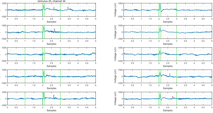
Remarkable is the low PPV. The number of false positive detections (median: 1897, range: 1840-1963) was high in each optimal setting. In Figure 3.11, an example of a true positive, true negative, false positive and false negative detection are displayed. The true positive detection is clearly an ER. The true negative detection shows a response after the specific time window for detecting ERs. Between the two vertical lines, no clear activity is visible. The false positive detection shows a large peak in the time window for ERs. This raises the question whether the visual annotation in this epoch was correct. Most false positive detections in the three patients may be reconsidered as ERs. Therefore, it is assumed that the actual number of false positive detections is lower than the current number.

(38)

Samples

0 10002000 30004000 50006000 70008000 9000 10000

Voltage (uV) -1000 -800 -600 -400 -200 0 200 400 600 800

1000 Trial 8, electrode 31

(a)A True Positive detection

Samples

0 1000 20003000 400050006000 70008000 9000 10000

Voltage (uV) -1000 -800 -600 -400 -200 0 200 400 600 800

(b)A True Negative detection

Samples

0 10002000 30004000 50006000 70008000 9000 10000

Voltage (uV) -1000 -800 -600 -400 -200 0 200 400 600 800

(c)A False Positive detection according to

the visual annotation. However, there is a clear response visible in the time window of an ER, so this may be recon-sidered.

Samples

0 1000 20003000 400050006000 70008000 9000 10000

Voltage (uV) -1000 -800 -600 -400 -200 0 200 400 600 800

(d)A False Negative detection

Figure 3.11:The two lines show the time window in which a peak must be present to be detected as an ER. When the first line is green, an ER was visually annotated. When the first line is red, no ER was annotated. The second line is green when an ER is detected and red when no ER is detected.

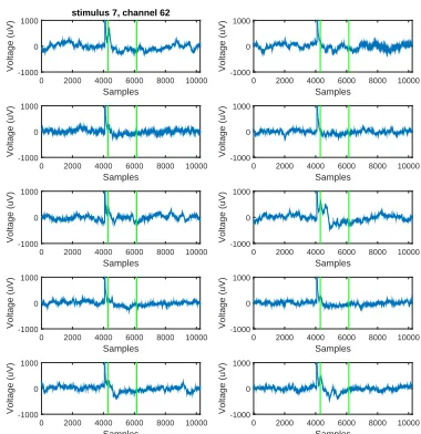
and slow waves were visible more than 100 ms after the stimulation artifact in the averaged epoch. So, it is doubtful that these peaks are delayed responses which occur only stochastic. To investigate whether these peaks are actual ERs is outside the scope of this study.

(39)

Samples

0 2000 4000 6000 8000 10000

Voltage (uV) -500 0 500 1000 1500 2000 2500 3000

Trial 35, electrode 27, SD ratio = -8.5

Samples

0 2000 4000 6000 8000 10000

Voltage (uV) -500 0 500 1000 1500 2000 2500 3000

Samples

0 2000 4000 6000 8000 10000

Voltage (uV) -500 0 500 1000 1500 2000 2500 3000

Figure 3.12:These electrodes show a response after the pulse. However, the peak occurs after 100 ms (the first figure) or it is not a peak or slow wave, but a lower plateau level (second and third figure). It is doubtful whether these responses should be detected as early responses.

Samples

0 10002000 30004000 50006000 70008000 9000 10000

Voltage (uV) -1000 -800 -600 -400 -200 0 200 400 600 800

1000 Stimulus 8, channel 8

(a)A False Positive detection in the

detec-tor with setting A1.

Samples

0 1000 20003000 40005000 60007000 80009000 10000

Voltage (uV) -1000 -800 -600 -400 -200 0 200 400 600 800

(b)A True Negative detection in the

detec-tor with setting B1.

Samples

0 10002000 30004000 50006000 70008000 9000 10000

Voltage (uV) -1000 -800 -600 -400 -200 0 200 400 600 800

(c)A False Negative detection in the

detec-tor with setting A1.

Samples

0 1000 20003000 40005000 60007000 80009000 10000

Voltage (uV) -1000 -800 -600 -400 -200 0 200 400 600 800

(d)A True Positive detection in the detector

with setting B1.

(40)

3.3 Validating the ER detector

3.3.1 Introduction

In the previous section, four ER detectors were tested in three patients. The performances of these detectors were comparable, but we concluded that the detector with setting B1, SD factor = 2.5, sel = 20

µV, minimal SD = 50µV was the best. In this section, this detector is validated. For this ER detector,

both the specificity and sensitivity must be high to construct a functional network. Our final goal is to discard stimulus pairs which will not evoke any DRs by the physiological network based on ERs. Since we do not want to falsely discard any stimulus pairs, it is important to avoid false negative detections. Therefore, sensitivity must be as high as possible.

3.3.2 Method

Visual annotation In three patients, ERs are annotated visually by DvB using Micromed, SystemPlus

Evolution with 5 s/page, no additional software filtering, and variable scaling (usually 1200µV/cm),

depending on the amplitude of the signals and the number of electrodes shown in the display. When amplitudes are too high to be able to differentiate ERs in neighboring electrodes, the scaling is decreased

to 2000µV/cm.

Detector In three patients, ERs are detected with the ER detector with B1 settings, SD factor = 2.5, sel

= 20µV, and minimal SD = 50µV. The number of true positive, false positive, true negative and false

negative ERs are determined based on comparison with visual annotations. Sensitivity, specificity, NPV and PPV (Formulas 3.1, 3.2, 3.3, 3.4 in chapter 3.1.2 are calculated in each patient to determine whether the detector is performing good enough for further usage.

3.3.3 Results

The validation set contained three patients (Table 3.4): 2 males and 1 female with an average age of 12 years old (mean: 776 per patient, range: 7-16). The ECoG data was recorded in February and March 2015. In total, 1564 ERs were annotated (mean: 819 per patient, range: 617-946). The detector detected 2458 ERs (range: 643-1112). The sensitivity, specificity, PPV and NPV are displayed in Table 3.5.

Table 3.4:Patient characteristics of validation set

Patient Gender Age Electrodes Trials Visual ERs Detected ERs

(per trial: median, range) (per trial: median, range)

89 f 14 56 45 764 (17, 7-28) 643 (15, 4-24)

91 m 16 86 54 617 (13, 4-26) 703 (13.5, 1-30)

93 m 7 64 48 946 (20, 0-33) 1112 (22.5, 0-42)

Table 3.5:The sensitivity, specificity, PPV and NPV for patients in the validation set

detector B1

Patient Sensitivity Specificity PPV NPV

89 0.71 0.94 0.84 0.88

91 0.76 0.94 0.67 0.96

93 0.86 0.86 0.73 0.93

(41)

3.3.4 Discussion

The mean sensitivity, specificity, PPV and NPV with the set variables in detector B1 were respectively 0.78, 0.91, 0.75, 0.92. Both the sensitivity and specificity are high. This means that most detected ERs are true ERs and not many ERs are missed. This is required for reconstructing a reliable physiological network. The sensitivity is not as high as the specificity. For now, we conclude that the ER detector performs sufficient to be used in further research. However, to reduce false negative detections, the ER detector must be improved before it may be used in a clinical setting.

A limitation of this study is that the visual annotations were only evaluated by DvB. No second observer had corroborated the annotations. Therefore, it is possible that ERs are wrongly annotated, missed or equivocal, so that the gold standard fails. Human scoring is by definition subjective. It is recommended that for further research, these annotations are determined by consensus between at least two observers. Another limitation is that we try to reconstruct a physiological network out of ERs. As thousands of cells are located under each electrode of the grid, it is likely that only strong and fast connections are revealed and some connections remain undetected. Although the presence of ERs provides evidence of connections between the electrodes to which a pulse is applied and the areas where they are recorded, the absence of ERs does not imply lack of functional connection [20]. There might be significant spread of neuronal impulses, e.g. due to polysynaptic pathways, which may render responses undetectable by SPES [20].

The network is based on the presence of an ER. The strength of an ER [24] and its delay [31] could also be very important for the reconstruction of the physiological network. This may be a good focus for further research. The current ER detector is only the first step in evaluating the presence of ERs and its physiological network.

A lot of research is done on diffusion tensor imaging (DTI) in the last couple of years. With diffusion imaging methods and tractography algorithms, trajectories of white-matter fascicles (tracts) in the human brain can be estimated in vivo [32]. Such methods could help in getting more insight in the physiological networks below the electrode grid and across the rest of the brain . We conclude that this ER detector is a good first step in analyzing the network of ERs in individual patients. The performance

of the ER detector with settings B1, SD factor = 2.5, sel = 20µV, and minimal SD = 50µV was sufficient

(42)

(43)

Improving the SPES protocol by automating ER and DR detection and evaluation of the spatial relation between ERs and DRs

U

niversity of

T

wente

M

aster

T

hesis

T

echnical

M

edicine

Improving the SPES protocol by automating ER

and DR detection and evaluation of the spatial

relation between ERs and DRs

Dorien van Blooijs

Contents

Chapter 1

1.1

Epilepsy

1.2

Surgery

1.3

Single Pulse Electrical Stimulation

1.4

Current situation

1.4.1

Acquisition of the SPES protocol

1.4.2

Analysis of responses

Chapter 2

2.1

Analysis of responses

2.1.1

Pre-processing

2.1.2

Early responses

2.1.3

Delayed responses

2.2

Acquisition of the SPES protocol

2.3

Stimulation settings of the SPES protocol

2.4

Other work

2.4.1

Abstracts

2.4.2

METC

Chapter 3

3.1

Constructing the ER detector

3.1.1

Introduction

3.1.2

Method

3.1.3

Results

3.1.4

Discussion

3.2

Evaluating the ER detector

3.2.1

Introduction

3.2.2

Method

3.2.3

Results

3.2.4

Discussion

3.3

Validating the ER detector

3.3.1

Introduction

3.3.2

Method

3.3.3

Results

3.3.4