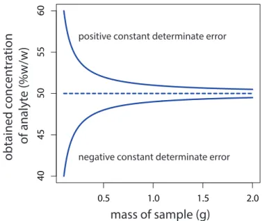
0.0 0.2 0.4 0.6 0.8 1.0 0.0 0.2 0.4 0.6 0.8 1.0 metal in e xcess ligand in e xcess XL absor banc e stoichiometric mixture
2.1
In
–HIn
pH = pK
a,HInindicator’s
color transition
range
indicator
is color of In
–indicator
is color of HIn
pH
2.95 3.00 3.05 3.10 3.15 3.20 3.25 Mass of Pennies (g) Phase 2 Phase 1An
aly
tical
C
hemistr
y
Print Version
Modern Analytical Chemistry by David Harvey
ISBN 0–07–237547–7
Copyright © 2000 by McGraw-Hill Companies
Copyright transferred to David Harvey, February 15, 2008
Electronic Versions
Analytical Chemistry 2.0 by David Harvey (fall 2009)
Analytical Chemistry 2.1 by David Harvey (summer 2016)
Copyright
This work is licensed under the Creative Commons Attribution-NonCommercial-ShareAlike 4.0 Unported License. To view a copy of this license, visit http://creativecommons.org/licenses/by-nc-sa/4.0/. Under the conditions of this copyright you are free to share this work with others in any medium or format. You also are free to remix, transform, and bulid upon this material provided that you attribute the original work and author and that you distribute your work under the same licence. You may not use this work for commercial purposes.
Illustrations and Photographs
Unless otherwise indicated, all illustrations and photographs are original to this text and are covered by the copyright described in the previous section. Other illustrations are in the public domain or are have a copyright under one or more variants of a GNU or Creative Commons license. For reused content, a hyperlink in the figure caption provides a link to the original source. Click here for a list of reused illustrations and the specific copyright information.
Brief Table of Contents
Preface . . . . xvii
Introduction to Analytical Chemistry . . . . 1
Basic Tools of Analytical Chemistry . . . . 13
The Vocabulary of Analytical Chemistry . . . . 41
Evaluating Analytical Data . . . . 63
Standardizing Analytical Methods . . . . 147
Equilibrium Chemistry . . . . 201
Collecting and Preparing Samples . . . . 271
Gravimetric Methods . . . . 337
Titrimetric Methods . . . . 391
Spectroscopic Methods . . . . 517
Electrochemical Methods . . . . 637
Chromatographic and Electrophoretic Methods . . . . 747
Kinetic Methods . . . . 847
Developing a Standard Method . . . . 905
Quality Assurance . . . . 953
Additional Resources . . . . 979
Appendix . . . . 1035
1 .
2 .
3 .
4 .
5 .
6 .
7 .
8 .
9 .
10 .
11 .
12 .
13 .
14 .
15 .
Detailed Table of Contents
Preface . . . . xvii
A Organization . . . xviii
B Role of Equilibrium Chemistry . . . xviii
C Computational Software . . . xix
D How to Use The Electronic Textbook’s Features. . . xix
E Acknowledgments . . . xxi
F Updates, Ancillary Materials, and Future Editions . . . xxiii
G How To Contact the Author . . . xxiii
Introduction to Analytical Chemistry . . . . 1
1A What is Analytical Chemistry? . . . .2
1B The Analytical Perspective . . . .5
1C Common Analytical Problems . . . .7
1D Key Terms . . . .8
1E Chapter Summary . . . .8
1F Problems . . . .9
1G Solutions to Practice Exercises . . . .10
Basic Tools of Analytical Chemistry . . . . 13
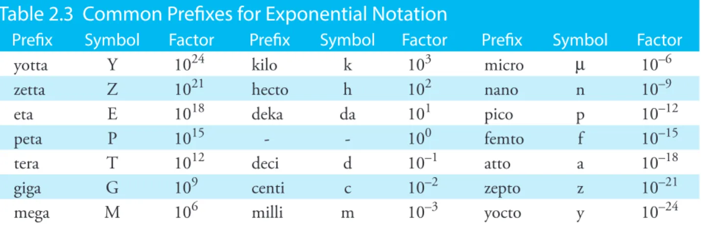
2A Measurements in Analytical Chemistry . . . .14
2A.1 Units of Measurement . . . 14
2A.2 Uncertainty in Measurements . . . 16
2B Concentration . . . .18
2B.1 Molarity and Formality . . . 19
2B.2 Normality . . . 20
2B.3 Molality . . . 20
2B.4 Weight, Volume, and Weight-to-Volume Percents . . . 20
2B.5 Parts Per Million and Parts Per Billion . . . 20
2B.6 Converting Between Concentration Units . . . 21
2B.7 p-Functions . . . 21
2C Stoichiometric Calculations . . . .23
2D Basic Equipment . . . .25
2D.1 Equipment for Measuring Mass . . . 26
2D.2 Equipment for Measuring Volume . . . 26
2D.3 Equipment for Drying Samples . . . 29
2E Preparing Solutions . . . .29
2E.1 Preparing Stock Solutions. . . 30
2G The Laboratory Notebook . . . .33
2H Key Terms . . . .34
2I Chapter Summary. . . .34
2J Problems . . . .34
2K Solutions to Practice Exercises . . . .37
The Vocabulary of Analytical Chemistry . . . . 41
3A Analysis, Determination and Measurement . . . .42
3B Techniques, Methods, Procedures, and Protocols . . . .43
3C Classifying Analytical Techniques . . . .44
3D Selecting an Analytical Method . . . .45
3D.1 Accuracy . . . 45
3D.2 Precision . . . 46
3D.3 Sensitivity . . . 46
3D.4 Specificity and Selectivity . . . 47
3D.5 Robustness and Ruggedness. . . 50
3D.6 Scale of Operation . . . 50
3D.7 Equipment, Time, and Cost . . . 52
3D.8 Making the Final Choice . . . 52
3E Developing the Procedure . . . .53
3E.1 Compensating for Interferences . . . 53
3E.2 Calibration . . . 54
3E.3 Sampling . . . 54
3E.4 Validation. . . 55
3F Protocols . . . .55
3G The Importance of Analytical Methodology . . . .56
3H Key Terms . . . .57
3I Chapter Summary. . . .57
3J Problems . . . .58
3K Solutions to Practice Exercises . . . .61
Evaluating Analytical Data . . . . 63
4A Characterizing Measurements and Results . . . .64
4A.1 Measures of Central Tendency . . . 64
4A.2 Measures of Spread . . . 66
4B Characterizing Experimental Errors . . . .68
4B.1 Errors That Affect Accuracy . . . 68
4B.2 Errors That Affect Precision . . . 73
4B.3 Error and Uncertainty . . . 75
4C Propagation of Uncertainty . . . .76
4C.3 Uncertainty When Multiplying or Dividing . . . 78
4C.4 Uncertainty for Mixed Operations . . . 78
4C.5 Uncertainty for Other Mathematical Functions . . . 79
4C.6 Is Calculating Uncertainty Actually Useful? . . . 81
4D The Distribution of Measurements and Results . . . .82
4D.1 Populations and Samples . . . 83
4D.2 Probability Distributions for Populations . . . 83
4D.3 Confidence Intervals for Populations . . . 89
4D.4 Probability Distributions for Samples . . . 91
4D.5 Confidence Intervals for Samples . . . 95
4D.6 A Cautionary Statement . . . 96
4E Statistical Analysis of Data . . . .97
4E.1 Significance Testing . . . 97
4E.2 Constructing a Significance Test . . . 98
4E.3 One-Tailed and Two-Tailed Significance Tests . . . 99
4E.4 Errors in Significance Testing . . . 100
4F Statistical Methods for Normal Distributions . . . .101
4F.1 Comparing X to n . . . 101
4F.2 Comparing s2 to v2 . . . 103
4F.3 Comparing Two Sample Variances . . . 104
4F.4 Comparing Two Sample Means . . . 105
4F.5 Outliers . . . 112
4G Detection Limits . . . .115
4H Using Excel and R to Analyze Data . . . .117
4H.1 Excel . . . 117
4H.2 R . . . 120
4I Key Terms . . . .128
4J Chapter Summary . . . .129
4K Problems . . . .129
4L Solutions to Practice Exercises . . . .139
Standardizing Analytical Methods . . . . 147
5A Analytical Standards. . . .148
5A.1 Primary and Secondary Standards . . . 148
5A.2 Other Reagents . . . 148
5A.3 Preparing a Standard Solution . . . 149
5B Calibrating the Signal (S
total) . . . .150
5C Determining the Sensitivity (k
A) . . . .150
5C.1 Single-Point versus Multiple-Point Standardizations . . . 151
5C.2 External Standards . . . 152
5C.3 Standard Additions . . . 155
5D.1 Linear Regression of Straight Line Calibration Curves . . . 164
5D.2 Unweighted Linear Regression with Errors in y . . . 164
5D.3 Weighted Linear Regression with Errors in y . . . 174
5D.4 Weighted Linear Regression with Errors in Both x and y . . . 177
5D.5 Curvilinear and Multivariate Regression . . . 177
5E Compensating for the Reagent Blank (S
reag) . . . .178
5F Using Excel and R for a Regression Analysis . . . .180
5F.1 Excel . . . 180
5F.2 R . . . 184
5G Key Terms . . . .189
5H Chapter Summary . . . .189
5I Problems . . . .190
5J Solutions to Practice Exercises . . . .194
Equilibrium Chemistry . . . . 201
6A Reversible Reactions and Chemical Equilibria . . . .202
6B Thermodynamics and Equilibrium Chemistry . . . .203
6C Manipulating Equilibrium Constants . . . .205
6D Equilibrium Constants for Chemical Reactions . . . .206
6D.1 Precipitation Reactions . . . 206
6D.2 Acid–Base Reactions . . . 206
6D.3 Complexation Reactions . . . 211
6D.4 Oxidation–Reduction (Redox) Reactions . . . 213
6E Le Châtelier’s Principle . . . .216
6F Ladder Diagrams . . . .218
6F.1 Ladder Diagrams for Acid–Base Equilibria . . . 219
6F.2 Ladder Diagrams for Complexation Equilibria . . . 222
6F.3 Ladder Diagram for Oxidation/Reduction Equilibria . . . 224
6G Solving Equilibrium Problems . . . .225
6G.1 A Simple Problem—Solubility of Pb(IO3)2 . . . 226
6G.2 A More Complex Problem—The Common Ion Effect . . . 227
6G.3 A Systematic Approach to Solving Equilibrium Problems . . . 229
6G.4 pH of a Monoprotic Weak Acid . . . 231
6G.5 pH of a Polyprotic Acid or Base . . . 233
6G.6 Effect of Complexation on Solubility . . . 235
6H Buffer Solutions . . . .237
6H.1 Systematic Solution to Buffer Problems . . . 238
6H.2 Representing Buffer Solutions with Ladder Diagrams . . . 240
6H.3 Preparing a Buffer . . . 241
6I Activity Effects . . . .242
6J.2 R . . . 251
6K Some Final Thoughts on Equilibrium Calculations . . . .254
6L Key Terms . . . .255
6M Chapter Summary . . . .255
6N Problems . . . .257
6O Solutions to Practice Exercises . . . .260
Collecting and Preparing Samples . . . . 271
7A The Importance of Sampling . . . .272
7B Designing A Sampling Plan . . . .275
7B.1 Where to Sample the Target Population . . . 275
7B.2 What Type of Sample to Collect . . . 279
7B.3 How Much Sample to Collect . . . 281
7B.4 How Many Samples to Collect . . . 283
7B.5 Minimizing the Overall Variance . . . 285
7C Implementing the Sampling Plan . . . .287
7C.1 Solutions . . . 287
7C.2 Gases . . . 289
7C.3 Solids . . . 291
7D Separating the Analyte from Interferents . . . .297
7E General Theory of Separation Efficiency . . . .297
7F Classifying Separation Techniques . . . .300
7F.1 Separations Based on Size . . . 300
7F.2 Separations Based on Mass or Density . . . 302
7F.3 Separations Based on Complexation Reactions (Masking) . . . 304
7F.4 Separations Based on a Change of State . . . 306
7F.5 Separations Based on a Partitioning Between Phases . . . 309
7G Liquid–Liquid Extractions . . . .314
7G.1 Partition Coefficients and Distribution Ratios . . . 314
7G.2 Liquid–Liquid Extraction With No Secondary Reactions . . . 315
7G.3 Liquid–Liquid Extractions Involving Acid–Base Equilibria . . . 318
7G.4 Liquid–Liquid Extraction of a Metal–Ligand Complex . . . 320
7H Separation Versus Preconcentration . . . .323
7I Key Terms . . . .323
7K Problems . . . .324
Gravimetric Methods . . . . 337
8A Overview of Gravimetric Methods . . . .338
8A.1 Using Mass as an Analytical Signal . . . 338
8A.2 Types of Gravimetric Methods . . . 339
8B Precipitation Gravimetry . . . .340
8B.1 Theory and Practice . . . 340
8B.2 Quantitative Applications . . . 354
8B.2 Qualitative Applications . . . 361
8B.3 Evaluating Precipitation Gravimetry. . . 361
8C Volatilization Gravimetry . . . .362
8C.1 Theory and Practice . . . 362
Thermogravimetry . . . 363
8C.2 Quantitative Applications . . . 367
8C.3 Evaluating Volatilization Gravimetry . . . 370
8D Particulate Gravimetry . . . .371
8D.1 Theory and Practice . . . 371
8D.2 Quantitative Applications . . . 373
8D.3 Evaluating Particulate Gravimetry . . . 374
8E Key Terms . . . .375
8F
Chapter Summary . . . .375
8G Problems . . . .375
8H Solutions to Practice Exercises . . . .385
Titrimetric Methods . . . . 391
9A Overview of Titrimetry . . . .392
9A.1 Equivalence Points and End points . . . 392
9A.2 Volume as a Signal . . . 392
9A.3 Titration Curves . . . 394
9A.4 The Buret . . . 395
9B Acid–Base Titrations . . . .396
9B.1 Acid–Base Titration Curves . . . 398
9B.2 Selecting and Evaluating the End Point . . . 406
9B.3 Titrations in Nonaqueous Solvents . . . 414
9B.5 Qualitative Applications . . . 428
9B.6 Characterization Applications . . . 429
9B.7 Evaluation of Acid–Base Titrimetry . . . 432
9C Complexation Titrations . . . .437
9C.1 Chemistry and Properties of EDTA . . . 437
9C.2 Complexometric EDTA Titration Curves . . . 440
9C.3 Selecting and Evaluating the End point . . . 445
9C.4 Quantitative Applications . . . 450
9C.5 Evaluation of Complexation Titrimetry . . . 454
9D Redox Titrations . . . .455
9D.1 Redox Titration Curves . . . 456
9D.2 Selecting and Evaluating the End point . . . 461
9E Precipitation Titrations . . . .478
9E.1 Titration Curves . . . 478
9E.2 Selecting and Evaluating the End point . . . 480
9E.3 Quantitative Applications. . . 482
9E.4 Evaluation of Precipitation Titrimetry . . . 485
9F Key Terms . . . .486
9G Chapter Summary . . . .486
9H Problems . . . .487
9I Solutions to Practice Exercises . . . .502
Spectroscopic Methods . . . . 517
10A Overview of Spectroscopy . . . .518
10A.1 What is Electromagnetic Radiation . . . 518
10A.2 Photons as a Signal Source . . . 521
10A.3 Basic Components of Spectroscopic Instruments . . . 523
Signal Processors . . . 530
10B Spectroscopy Based on Absorption . . . .530
10B.1 Absorbance Spectra . . . 530
10B.2 Transmittance and Absorbance . . . 535
10B.3 Absorbance and Concentration: Beer’s Law . . . 537
10B.4 Beer’s Law and Multicomponent Samples . . . 538
10B.5 Limitations to Beer’s Law . . . 538
10C UV/Vis and IR Spectroscopy . . . .540
10C.1 Instrumentation . . . 540
10C.2 Quantitative Applications . . . 548
10C.3 Qualitative Applications . . . 560
10C.4 Characterization Applications . . . 562
10C.5 Evaluation of UV/Vis and IR Spectroscopy . . . 568
10D Atomic Absorption Spectroscopy . . . .572
10D.1 Instrumentation . . . 572
10D.2 Quantitative Applications . . . 576
10D.3 - Evaluation of Atomic Absorption Spectroscopy . . . 583
10E Emission Spectroscopy . . . .585
10F Photoluminescence Spectroscopy . . . .585
10F.1 Fluorescence and Phosphorescence Spectra . . . 586
10F.2 Instrumentation . . . 590
10F.3 Quantitative Applications . . . 593
10F.4 Evaluation of Photoluminescence Spectroscopy . . . 597
10G Atomic Emission Spectroscopy . . . .599
10G.1 Atomic Emission Spectra . . . 599
10G.2 Equipment . . . 600
10H Spectroscopy Based on Scattering . . . .608
10H.1 Origin of Scattering. . . 608
10H.2 Turbidimetry and Nephelometry . . . 609
10I Key Terms . . . .615
10J Chapter Summary . . . .616
10K Problems . . . .617
10L Solutions to Practice Exercises . . . .634
Electrochemical Methods . . . . 637
11A Overview of Electrochemistry . . . .638
11A.2 Five Important Concepts . . . 638
11A.2 Controlling and Measuring Current and Potential . . . 640
11A.3 Interfacial Electrochemical Techniques . . . 643
11B Potentiometric Methods . . . .644
11B.1 Potentiometric Measurements . . . 645
11B.2 Reference Electrodes . . . 651
11B.3 Metallic Indicator Electrodes . . . 655
11B.4 Membrane Electrodes . . . 656 11B.5 Quantitative Applications . . . 669 11B.6 Evaluation . . . 678
11C Coulometric Methods . . . .681
11C.1 Controlled-Potential Coulometry . . . 681 11C.2 Controlled-Current Coulometry . . . 684 11C.3 Quantitative Applications . . . 687 11C.4 Characterization Applications . . . 693 11C.5 - Evaluation . . . 69411D Voltammetric Methods . . . .696
11D.1 Voltammetric Measurements . . . 696 11D.2 Current in Voltammetry . . . 698 11D.3 Shape of Voltammograms . . . 70311D.4 Quantitative and Qualitative Aspects of Voltammetry . . . 703
11D.5 Voltammetric Techniques . . . 705
11D.6 Quantitative Applications . . . 714
11D.7 Characterization Applications . . . 722
11D.8 Evaluation . . . 726
11E Key Terms . . . .727
11F Chapter Summary . . . .728
11G Problems . . . .729
11H Solutions to Practice Exercises . . . .742
Chromatographic and Electrophoretic Methods . . . . 747
12A.2 A Better Way to Separate Mixtures . . . 748
12A.3 Chromatographic Separations . . . 751
12A.4 Electrophoretic Separations . . . 752
12B General Theory of Column Chromatography . . . .753
12B.1 Chromatographic Resolution . . . 755
12B.2 Solute Retention Factor . . . 756
12B.3 Selectivity . . . 759
12B.4 Column Efficiency . . . 759
12B.5 Peak Capacity . . . 761
12B.6 Asymmetric Peaks . . . 761
12C Optimizing Chromatographic Separations. . . .762
12C.1 Using the Retention factor to Optimize Resolution . . . 763
12C.2 Using Selectivity to Optimize Resolution . . . 765
12C.3 Using Column Efficiency to Optimize Resolution . . . 766
12D Gas Chromatography . . . .770
12D.1 Mobile Phase . . . 771
12D.2 Chromatographic Columns . . . 771
12D.3 Sample Introduction . . . 774
12D.4 Temperature Control . . . 778
12D.5 Detectors for Gas Chromatography . . . 778
12D.6 Quantitative Applications . . . 781
12D.7 Qualitative Applications . . . 785
12D.8 Evaluation . . . 789
12E High-Performance Liquid Chromatography . . . .790
12E.1 HPLC Columns . . . 790
12E.2 Mobile Phases . . . 793
12E.3 HPLC Plumbing . . . 797
12E.4 Detectors for HPLC . . . 799
12E.5 Quantitative Applications. . . 803
12E.6 Evaluation . . . 806
12F Other Forms of Liquid Chromatography . . . .806
12F.1 Liquid-Solid Adsorption Chromatography . . . 807
12F.2 Ion-Exchange Chromatography . . . 807
12F.3 Size-Exclusion Chromatography . . . 810
12F.4 Supercritical Fluid Chromatography . . . 812
12G Electrophoresis . . . .814
12G.1 Theory of Capillary Electrophoresis . . . 814
12G.2 Instrumentation . . . 819
12G.3 Capillary Electrophoresis Methods . . . 823
12G.4 Evaluation . . . 828
12H Key Terms . . . .828
12K Solutions to Practice Exercises . . . .842
Kinetic Methods . . . . 847
13A Kinetic Methods Versus Equilibrium Methods . . . .848
13B Chemical Kinetics . . . .849
13B.1 Theory and Practice . . . 849
13B.2 Classifying Chemical Kinetic Methods . . . 851
13B.3 Making Kinetic Measurements . . . 861
13B.4 Quantitative Applications . . . 863
13B.5 Characterization Applications . . . 866
13B.6 Evaluation of Chemical Kinetic Methods . . . 870
Accuracy . . . 870
13C Radiochemistry . . . .873
13C.1 Theory and Practice . . . 874
13C.2 Instrumentation . . . 875
13C.3 Quantitative Applications . . . 875
13C.4 Characterization Applications . . . 879
13C.5 Evaluation . . . 880
13D Flow Injection Analysis . . . .881
13D.1 Theory and Practice . . . 881
13D.2 Instrumentation . . . 884
13D.3 Quantitative Applications . . . 889
13D.4 Evaluation . . . 893
13E Key Terms . . . .894
13F Summary . . . .894
13G Problems . . . .895
13H Solutions to Practice Exercises . . . .903
Developing a Standard Method . . . . 905
14A Optimizing the Experimental Procedure . . . .906
14A.1 Response Surfaces . . . 906
14A.2 Searching Algorithms for Response Surfaces . . . 907
14A.3 Mathematical Models of Response Surfaces . . . 914
14B Verifying the Method . . . .923
14B.1 Single Operator Characteristics . . . 923
14B.2 Blind Analysis of Standard Samples . . . 924
14B.3 Ruggedness Testing . . . 924
14B.4 Equivalency Testing . . . 927
14C Validating the Method as a Standard Method . . . .927
14C.1 Two-Sample Collaborative Testing . . . 928
14C.2 Collaborative Testing and Analysis of Variance . . . 932
14D.1 Excel . . . 939
14D.2 R . . . 940
14E Key Terms . . . .942
14F Summary . . . .942
14G Problems . . . .943
14H Solutions to Practice Exercises . . . .951
Quality Assurance . . . . 953
15A The Analytical Perspective—Revisited . . . .954
15B Quality Control . . . .955
15C Quality Assessment . . . .957
15C.1 Internal Methods of Quality Assessment . . . 957
15C.2 External Methods of Quality Assessment . . . 961
15D Evaluating Quality Assurance Data . . . .962
15D.1 Prescriptive Approach . . . 962
15D.2 Performance-Based Approach . . . 965
15E Key Terms . . . .972
15F Chapter Summary . . . .972
15G Problems . . . .973
15H Solutions to Practice Exercises . . . .976
Additional Resources . . . . 979
Chapter 1 . . . .980
Chapter 2 . . . .982
Chapter 3 . . . .983
Chapter 4 . . . .984
Chapter 5 . . . .989
Chapter 6 . . . .993
Chapter 7 . . . .996
Chapter 8 . . . .1000
Chapter 9 . . . .1001
Chapter 10 . . . .1004
Chapter 11 . . . .1012
Chapter 12 . . . .1017
Chapter 13 . . . .1024
Chapter 14 . . . .1027
Chapter 15 . . . .1029
Appendix 1: Normality . . . .1036
Appendix 2: Propagation of Uncertainty . . . .1037
Standardizing a Solution of NaOH . . . 1037
Identifying and Analyzing Sources of Uncertainty . . . 1037
Estimating the Standard Deviation for Measurements . . . 1039
Completing the Propagation of Uncertainty . . . 1039
Evaluating the Sources of Uncertainty . . . 1042
Appendix 3: Single-Sided Normal Distribution . . . .1043
Appendix 4: Critical Values for t-Test . . . .1045
Appendix 5: Critical Values for the F-Test . . . .1046
Appendix 6: Critical Values for Dixon’s Q-Test . . . .1048
Appendix 7: Critical Values for Grubb’s Test . . . .1049
Appendix 8: Recommended Primary Standards . . . .1050
Appendix 9: Correcting Mass
for the Buoyancy of Air . . . .1052
Appendix 10: Solubility Products . . . .1054
Appendix 11: Acid Dissociation Constants . . . .1058
Appendix 12: Formation Constants . . . .1066
Appendix 13: Standard Reduction Potentials . . . .1071
Appendix 14: Random Number Table . . . .1080
Appendix 15: Polarographic
Half-Wave Potentials . . . .1081
Appendix 16: Countercurrent Separations . . . .1082
Appendix 17: Review of Chemical Kinetics . . . .1089
A17.1 Chemical Reaction Rates . . . 1089
A17.2 The Rate Law . . . 1089
A17.3 Kinetic Analysis of Selected Reactions . . . 1090
Appendix 18: Atomic Weights of the Elements . . . .1094
xvii
Preface
Preface
Overview
A
Organization
B
Role of Equilibrium Chemistry
C
Computational Software
D
How to Use The Electronic Textbook’s Features
E
Acknowledgments
F
Updates, Ancillary Materials, and Future Editions
G
How To Contact the Author
A
s currently taught in the United States, introductory courses in analytical chemistry emphasize quantitative (and sometimes qualitative) methods of analysis along with a heavy dose of equilibrium chemistry. Analytical chemistry, however, is much more than a collection of analytical methods and an understanding of equilibrium chemistry; it is an approach to solving chemical problems. Although equilibrium chemistry and analytical methods are important, their coverage should not come at the expense of other equally important topics. The introductory course in analytical chemistry is the ideal place in the undergraduate chemistry curriculum for exploring topics such as experimental design, sampling, calibration strategies, standardization, optimization, statistics, and the validation of experimental results. Analytical methods come and go, but best practices for designing and validating analytical methods are universal. Because chemistry is an experimental science it is essential that all chemistry students understand the importance of making good measurements.My goal in preparing this textbook is to find a more appropriate balance between theory and practice, between “classical” and “modern” analytical methods, between analyzing samples and collecting samples and preparing them for analysis, and between analytical methods and data analysis. There is more material here than anyone can cover in one semester; it is my hope that the diversity of topics will meet the needs of different instructors, while, perhaps, suggesting some new topics to cover.
A Organization
This textbook is organized into four parts. Chapters 1–3 serve as a general introduction, providing: an overview of analytical chemistry (Chapter 1); a review of the basic equipment and mathematical tools of analytical chem-istry, including significant figures, units, and stoichiometry (Chapter 2); and an introduction to the terminology of analytical chemistry (Chapter 3). Familiarity with this material is assumed throughout the remainder of the textbook.
Chapters 4–7 cover a number of topics that are important in under-standing how analytical methods work. Later chapters are mostly indepen-dent of these chapters, allowing an instructor to choose those topics that support his or her goals. Chapter 4 provides an introduction to the sta-tistical analysis of data. Methods for calibrating equipment and standard-izing methods are covered in Chapter 5, along with a discussion of linear regression. Chapter 6 provides an introduction to equilibrium chemistry, stressing both the rigorous solution to equilibrium problems and the use of semi-quantitative approaches, such as ladder diagrams. The importance of collecting the right sample, and methods for separating analytes and interferents are the subjects of Chapter 7.
Chapters 8–13 cover the major areas of analysis, including gravimetry (Chapter 8), titrimetry (Chapter 9), spectroscopy (Chapter 10), electro-chemistry (Chapter 11), chromatography and electrophoresis (Chapter 12), and kinetic methods (Chapter 13). Related techniques, such as acid–base titrimetry and redox titrimetry, are intentionally gathered together in single chapters. Combining related techniques in this way encourages students to see the similarity between methods, rather than focusing on their differ-ences. The first technique in each chapter is generally that which is most commonly covered in an introductory course.
Finally, the textbook concludes with two chapters discussing the design and maintenance of analytical methods, two topics of importance to all ex-perimental chemists. Chapter 14 considers the development of an analyti-cal method, including its optimization, its verification, and its validation. Quality control and quality assessment are discussed in Chapter 15.
B Role of Equilibrium Chemistry
Equilibrium chemistry often receives a significant emphasis in the intro-ductory analytical chemistry course. Although it is an important topic, an overemphasis on the computational aspects of equilibrium chemistry may lead students to confuse analytical chemistry with equilibrium chemistry. Solving equilibrium problems is important—it is equally important, how-ever, for students to recognize when such calculations are impractical, or to recognize when a simpler, more intuitive approach is all they need to answer a question. For example, in discussing the gravimetric analysis of Ag+ by precipitating AgCl, there is little point in calculating the
equilib-rium solubility of AgCl because the equilibequilib-rium concentration of Cl– is rarely known. It is important, however, for students to understand that a large excess of Cl– increases the solubility of AgCl due to the formation of soluble silver–chloro complexes. To balance the presentation of a rigorous approach to solving equilibrium problems, this textbook also introduces ladder diagrams as a means for rapidly evaluating the effect of solution conditions on an analysis. Students are encouraged to use the approach best suited to the problem at hand.
C Computational Software
Many of the topics in this textbook benefit from the availability of appro-priate computational software. There are many software packages available to instructors and students, including spreadsheets (e.g. Excel), numerical computing environments (e.g. Mathematica, Mathcad, Matlab, R), statisti-cal packages (e.g. SPSS, Minitab), and data analysis/graphing packages (e.g. Origin). Because of my familiarity with Excel and R, examples of their use in solving problems are incorporated into this textbook. Instructors inter-ested in incorporating other software packages into future editions of this textbook are encouraged to contact me at [email protected].
D How to Use The Electronic Textbook’s Features
As with any format, an electronic textbook has advantages and disadvan-tages. Perhaps the biggest disadvantage to an electronic textbook is that you cannot hold it in your hands (and I, for one, like the feel of book in my hands when reading) and leaf through it. More specifically, you cannot mark your place with a finger, flip back several pages to look at a table or figure, and then return to your reading when you are done. To overcome this limitation, an electronic textbook can make extensive use of hyperlinks. Whenever the text refers to an object that is not on the current page— a figure, a table, an equation, an appendix, a worked example, a practice exercise—the text is displayed in blue and is underlined. Clicking on the hyperlink transports you to the relevant object. There are two methods for returning to your original location within the textbook. When there is no ambiguity about where to return, such as when reviewing an answer to a practice exercise, a second text hyperlink is included.
Most objects have links from multiple places within the text, which means a single return hyperlink is not possible. To return to your original place select View: Go To: Previous View from the menu bar. If you do not like to use pull down menus, you can configure the toolbar to include but-tons for “Previous View” and for “Next View.” To do this, click on View: Toolbars: More Tools . . ., scroll down to the category for Page Navigation Tools and check the boxes for Previous View and for Next View. Your
toolbar now includes buttons that you can use to return to your original Click this button to return to your
original position within the text
Although you can use any PDF reader to read this electronic textbook, the use of Adobe’s Acrobat Reader is strongly encouraged. Several features of this elec-tronic textbook—notably the comment-ing tools and the inclusion of video—are available only when using Acrobat Reader 8.0 or later. If you do not have Acrobat Reader installed on your computer, you can obtain it from Adobe’s web site.
position within the text. These buttons will appear each time you open the electronic textbook.
There are several additional hyperlinks to help you navigate within the electronic textbook. The Table of Contents—both the brief form and the expanded form—provide hyperlinks to chapters, to main sections, and to subsections. The “Chapter Overview” on the first page of each chapter pro-vides hyperlinks to the chapter’s main sections. The textbook’s title, which appears at the top of each even numbered page, is a hyperlink to the brief table of contents, and the chapter title, which appears at the top of most odd numbered pages, is a hyperlink to the chapter’s first page. The collec-tion of key terms at the end of each chapter are hyperlinks to where the terms were first introduced, and the key terms in the text are hyperlinks that return you to the collection of key terms. Taken together, these hyper-links provide for a easy navigation.
If you are using Adobe Reader, you can configure the program to re-member where you were when you last closed the electronic textbook. Se-lect Adobe Reader: Preferences . . . from the menu bar. SeSe-lect the category “Documents” and check the box for “Restore last view settings when re-opening documents.” This is a global change that will affect all documents that you open using Adobe Reader.
There are two additional features of the electronic textbook that you may find useful. The first feature is the incorporation of QuickTime and Flash movies. Some movies are configured to run when the page is dis-played, and other movies include start, pause, and stop buttons. If you find that you cannot play a movie check your permissions. You can do this by selecting Adobe Reader: Preferences . . . from the menu bar. Choose the option for “Multimedia Trust” and check the option for “Allow multimedia operations.” If the permission for
QuickTime or Flash is set to “Never” you can change it to “Prompt,” which will ask you to authorize the use of multimedia when you first try to play the movie, or change it to “Always” if you do not wish to prevent any files from playing movies.
A second useful feature is the availability of Adobe’s commenting tools, which allow you to highlight text, to create text boxes in which you can type notes, to add sticky notes, and to attach files. You can access the com-menting tools by selecting Tools: Comcom-menting & Markup from the menu bar. If you do not like to use the menu bar, you can add tools to the tool bar by selecting View: Toolbars: Commenting & Markup from the menu bar. To control what appears on the toolbar, select View: Toolbars: More Tools . . . and check the boxes for the tools you find most useful. Details on some of the tools are shown here. You can alter any tool’s properties, such
as color, by right-clicking on the tool and selecting Tool Default Proper-ties . . . from the pop-up menu.
These tools allow you to highlight, to under-line, and to cross out text. Select the tool and the click and drag over the relevant text. The text box tool allows you to provide short
annotations to the textbook. Select the tool and then click and drag to create a text box. Click in the textbook and type your note. The sticky note tool is useful when you have a
longer annotation or when you want to make your annotation easier to see. Click in the textbook at the spot where you wish to add the sticky note. Type your entry and the click the close button to collapse the note into its icon. Hovering the cursor over the icon dis-plays the note and clicking on the icon allows you to edit your note.
The pencil tool allows you to use your mouse to write notes on the text. The eraser tool al-lows you to erase notes.
The paperclip tool allows you to attach a file to the textbook. Select the tool and click in the textbook at the spot where you wish to attach the file. Use the browser to find the file and select OK. The resulting icon is a link to the file. You can open the file by clicking on the icon.
E Acknowledgments
This textbook began as a print version published in 2000 by McGraw-Hill, and the support of the then editorial staff (Jim Smith, Publisher for Chemistry; Kent Peterson, Sponsoring Editor for Chemistry; Shirley Ober-broeckling, Developmental Editor for Chemistry; and Jayne Klein, Proj-ect Manager) is gratefully acknowledged. The assistance of Thomas Timp (Sponsoring Editor for Chemistry) and Tamara Hodge (Senior Sponsoring Editor for Chemistry) in returning the copyright to me also is acknowl-edged. The following individuals kindly reviewed portions of the print ver-sion as it worked its way through the publication process:
David Ballantine, Northern Illinois University John Bauer, Illinois State University
Ali Bazzi, University of Michigan–Dearborn
Christopher Harrison, a faculty member in the Chemistry Department at San Di-ego State University, has prepared instruc-tional videos that describe how to use Pre-view or Adobe Acrobrat Reader to work with pdf textbooks; you can use the links to view these videos.
Steven D. Brown, University of Delaware
Wendy Clevenger, University of Tennessee–Chattanooga Cathy Cobb, Augusta State University
Paul Flowers, University of North Carolina–Pembroke George Foy, York College of Pennsylvania
Nancy Gordon, University of Southern Maine Virginia M. Indivero, Swarthmore College Michael Janusa, Nicholls State University J. David Jenkins, Georgia Southern University David Karpovich, Saginaw Valley State University Gary Kinsel, University of Texas at Arlington John McBride, Hoftsra University
Richard S. Mitchell, Arkansas State University George A. Pearse, Jr., LeMoyne College Gary Rayson, New Mexico State University David Redfield, NW Nazarene University Vincent Remcho, West Virginia University Jeanette K. Rice, Georgia Southern University Martin W. Rowe, Texas A&M University Alexander Scheeline, University of Illinois James D. Stuart, University of Connecticut Thomas J. Wenzel, Bates College
David Zax, Cornell University
I am particularly grateful for their detailed comments and suggestions. Much of what is good in the print edition is the result of their interest and ideas.
Without the support of DePauw University and its Faculty Develop-ment Committee, work on this project would not have been possible. This project began in 1992 with a summer course development grant, and re-ceived further summer support from the President’s Discretionary Fund. Portions of the first draft were written during a sabbatical leave in fall 1993. The second draft was completed with the support of a Fisher Fellowship in fall 1995. Converting the print version into this electronic version was completed as part of a year-long sabbatical during the 2008/09 academic year. A full-year sabbatical during the 2015/16 academic year provided the time to complete a second edition.
The following faculty members and students graciously provided data for figures included in this textbook: Bridget Gourley, Jeanette Pope, and Daniel Scott (DePauw University), Michelle Bushey, Zoe LaPier, Christo-pher Schardon, and Kyle Meinhardt (Trinity University), and Dwight Stoll, Jason Schultz, Joanna Berry, and Kaelene Lundstrom (Gustavus Adolphus College).
I am grateful to the following individuals for their encouragement and support, for their camaraderie at curricular development workshops, or for their testing of draft versions of this eText: Cynthia Larive (University of
California–Riverside), Ted Kuwana (Kansas), Alex Scheeline (University of Illinois), Tom Spudich (United States Military Academy), Heather Bul-len (University of Northern Kentucky), Richard Kelly (East Stroudsburg University), William Otto (University of Maine–Machias), Alanah Fitch (Loyola University), Thomas Wenzel (Bates College), Anna Cavinato (East-ern Oregon University), Steve Petrovic (University of South(East-ern Oregon), Erin Gross (Creighton University), Mark Vitha (Drake University), Sara Choung (Point Loma Nazarene University), Michael Setter (John Carroll University), Corrine Lehr (California Polytechnic State University), Chris-topher Harrison (San Diego State University), and Bryan Hanson (DePauw University).
F Updates, Ancillary Materials, and Future Editions
The website for this eText provides access to both the current version ofthe textbook (Analytical Chemistry 2.1) and to legacy editions, including the eText’s illustrations. Also available through the website is a solutions manual and links to a variety of ancillary materials, including case studies, Shiny apps, and scripts and packages of functions for use with R. If you are interested in contributing problems, case studies, data sets, photographs, figures or any other content, please contact the author at harvey@depauw. edu.
G How To Contact the Author
Working on this textbook continues to be an interesting challenge and a rewarding endeavour. One interesting aspect of electronic publishing is that a book is not static—corrections, new examples and problems, and new topics are easy to add, and new editions released as needed. I welcome your input and encourage you to contact me with suggestions for improving this electronic textbook. You can reach me by e-mail at [email protected].
1
Chapter 1
Introduction to
Analytical Chemistry
Chapter Overview
1A What is Analytical Chemistry?
1B The Analytical Perspective
1C Common Analytical Problems
1D Key Terms
1E Chapter Summary
1F Problems
1G Solutions to Practice Exercises
C
hemistry is the study of matter, including its composition, its structure, its physical properties, and its reactivity. Although there are many ways to study chemistry, traditionally we divide it into five areas: organic chemistry, inorganic chemistry, biochemistry, physical chemistry, and analytical chemistry. This division is historical and, perhaps, arbitrary, as suggested by current interest in interdisciplinary areas, such as bioanalytical chemistry and organometallic chemistry. Nevertheless, these five areas remain the simplest division that spans the discipline of chemistry.Each of these traditional areas of chemistry brings a unique perspective to how a chemist makes sense of the diverse array of elements, ions, and molecules (both small and large) that make up our physical environment. An undergraduate chemistry course, therefore, is much more than a collection of facts; it is, instead, the means by which we learn to see the chemical world from a different perspective. In keeping with this spirit, this chapter introduces you to the field of analytical chemistry and highlights the unique perspectives that analytical chemists bring to the study of chemistry.
1A What is Analytical Chemistry?
“Analytical chemistry is what analytical chemists do.”
Let’s begin with a deceptively simple question: What is analytical chemis-try? Like all areas of chemistry, analytical chemistry is so broad in scope and so much in flux that it is difficult to find a simple definition more revealing than that quoted above. In this chapter we will try to expand upon this simple definition by saying a little about what analytical chemistry is, as well as a little about what analytical chemistry is not.
Analytical chemistry often is described as the area of chemistry respon-sible for characterizing the composition of matter, both qualitatively (Is there lead in this paint chip?) and quantitatively (How much lead is in this paint chip?). As we shall see, this description is misleading.
Most chemists routinely make qualitative and quantitative measure-ments. For this reason, some scientists suggest that analytical chemistry is not a separate branch of chemistry, but simply the application of chemical knowledge.1 In fact, you probably have performed many such quantitative
and qualitative analyses in other chemistry courses.
Defining analytical chemistry as the application of chemical knowledge ignores the unique perspective that an analytical chemist bring to the study of chemistry. The craft of analytical chemistry is found not in performing a routine analysis on a routine sample—a task we appropriately call chemical analysis—but in improving established analytical methods, in extending these analytical methods to new types of samples, and in developing new analytical methods to measure chemical phenomena.2
Here is one example of the distinction between analytical chemistry and chemical analysis. A mining engineers evaluates an ore by comparing the cost of removing the ore from the earth with the value of its contents, which they estimate by analyzing a sample of the ore. The challenge of developing and validating a quantitative analytical method is the analyti-cal chemist’s responsibility; the routine, daily application of the analytianalyti-cal method is the job of the chemical analyst.
Another difference between analytical chemistry and chemical analysis is that an analytical chemist works to improve and to extend established analytical methods. For example, several factors complicate the quantita-tive analysis of nickel in ores, including nickel’s unequal distribution within the ore, the ore’s complex matrix of silicates and oxides, and the presence of other metals that may interfere with the analysis. Figure 1.1 outlined one standard analytical method in use during the late nineteenth century.3 The
need for many reactions, digestions, and filtrations makes this analytical method both time-consuming and difficult to perform accurately.
1 Ravey, M. Spectroscopy, 1990, 5(7), 11. 2 de Haseth, J. Spectroscopy, 1990, 5(7), 11.
3 Fresenius. C. R. A System of Instruction in Quantitative Chemical Analysis; John Wiley and Sons: New York, 1881.
This quote is attributed to C. N. Reilly (1925-1981) on receipt of the 1965 Fish-er Award in Analytical Chemistry. Reilly, who was a professor of chemistry at the University of North Carolina at Cha-pel Hill, was one of the most influential analytical chemists of the last half of the twentieth century.
You might, for example, have determined the concentration of acetic acid in vinegar using an acid–base titration, or used a qual scheme to identify which of several metal ions are in an aqueous sample.
Seven Stages of an Analytical Method
1. Conception of analytical method (birth).
2. Successful demonstration that the analytical method works.
3. Establishment of the analytical meth-od’s capabilities.
4. Widespread acceptance of the analyti-cal method.
5. Continued development of the ana-lytical method leads to significant im-provements.
6. New cycle through steps 3–5. 7. Analytical method can no longer
com-pete with newer analytical methods (death).
Steps 1–3 and 5 are the province of ana-lytical chemistry; step 4 is the realm of chemical analysis.
The seven stages of an analytical method listed here are modified from Fassel, V. A. Fresenius’ Z. Anal. Chem. 1986, 324, 511–518 and Hieftje, G. M. J. Chem.
Educ. 2000, 77, 577–583.
For another view of what constitutes analytical chemistry, see the article “Quo Vadis, Analytical Chemistry?”, the full reference for which is Valcárcel, M. Anal.
Figure 1 .1 Fresenius’ analytical scheme for the gravimetric analysis of Ni in ores. After each step, the solid and the solution are separated by gravity filtration. Note that the mass of nickel is not determined directly. Instead, Co and Ni first are isolated and weighed together (mass A), and then Co is isolated and weighed separately (mass B). The timeline shows that it takes approximately 58 hours to analyze one sample. This scheme is an example of a gravimetric analysis, which is explored further in Chapter 8.
Original Sample
PbSO4; Sand
1:3 H2SO4/HNO3, 100°C for 8-10 hrs dilute w/H2O, digest for 2-4 hr
Cu2+, Fe3+, Co2+, Ni2+
dilute; bubble H2S(g)
CuS Fe3+, Co2+, Ni2+
cool, add NH3
digest 50o-70o for 30 min
Fe(OH)3 Co2+, Ni2+ HCl
Fe3+
neutralize w/NH3 add Na2CO3, CH3COOH
basic ferric acetate
Waste
slightly acidify w/HCl heat, bubble H2S(g)
CoS, NiS
add aqua regia and heat add HCl until strongly acidic bubble H2S(g)
Co2+, Ni2+ CuS, PbS
Waste Co(OH)2, Ni(OH)2
heat
add Na2CO3 until alkaline add NaOH
Co, Ni
heat; H2(g)
add HNO3, K2CO3, KNO3,
and CH3COOH and digest for 24 hours
Ni2+ K 3Co(NO3)5 add dilute HCl Waste Co2+ Co follow procedure from point * above
*
Solids Solutions
mass A
%Ni = mass A - mass B mass sample x 100 mass B key
A
ppr
o
xima
te Elapsed
T
ime
14 hours 16 hours 17 hours 20 hours 22 hours 23 hours 26 hours 51 hours 54 hours 58 hours Startdimethylglyoxime
The discovery, in 1905, that dimethylglyoxime (dmg) selectively precip-itates Ni2+ and Pd2+ led to an improved analytical method for the quantita-tive analysis of nickel.4 The resulting analysis, which is outlined in Figure
1.2, requires fewer manipulations and less time. By the 1970s, flame atomic absorption spectrometry replaced gravimetry as the standard method for analyzing nickel in ores,5 resulting in an even more rapid analysis. Today,
the standard analytical method utilizes an inductively coupled plasma opti-cal emission spectrometer.
Perhaps a more appropriate description of analytical chemistry is “the science of inventing and applying the concepts, principles, and…strategies for measuring the characteristics of chemical systems.”6 Analytical
chem-ists often work at the extreme edges of analysis, extending and improving 4 Kolthoff, I. M.; Sandell, E. B. Textbook of Quantitative Inorganic Analysis, 3rd Ed., The
Macmil-lan Company: New York, 1952.
5 Van Loon, J. C. Analytical Atomic Absorption Spectroscopy, Academic Press: New York, 1980. 6 Murray, R. W. Anal. Chem. 1991, 63, 271A.
Figure 1 .2 Gravimetric analysis for Ni in ores by precipitating Ni(dmg)2. The timeline shows that
it takes approximately 18 hours to analyze a single sample, substantially less than 58 hours for the method in Figure 1.1. The factor of 0.2301 in the equation for %Ni accounts for the difference in the formula weights of Ni and Ni(dmg)2; see Chapter 8 for further details.
Solids Solutions Original Sample HNO3, HCl, heat Residue Solution 20% NH4Cl 10% tartaric acid make alkaline w/ 1:1 NH3 Is solid present? yes no make acidic w/ HCl 1% alcoholic dmg make alkaline w/ 1:1 NH3 Ni(dmg)2 mass A %Ni = mass A x 0.2031 mass sample x 100
A
p
pr
o
xima
te Elaps
e
d
T
ime
Start 18 hours 14 hours key N OH CH3 CH3 N HOthe ability of all chemists to make meaningful measurements on smaller samples, on more complex samples, on shorter time scales, and on species present at lower concentrations. Throughout its history, analytical chemis-try has provided many of the tools and methods necessary for research in other traditional areas of chemistry, as well as fostering multidisciplinary research in, to name a few, medicinal chemistry, clinical chemistry, toxicol-ogy, forensic chemistry, materials science, geochemistry, and environmental chemistry.
You will come across numerous examples of analytical methods in this textbook, most of which are routine examples of chemical analysis. It is important to remember, however, that nonroutine problems prompted analytical chemists to develop these methods.
1B The Analytical Perspective
Having noted that each area of chemistry brings a unique perspective to the study of chemistry, let’s ask a second deceptively simple question: What is the analytical perspective? Many analytical chemists describe this perspec-tive as an analytical approach to solving problems.7 Although there likely
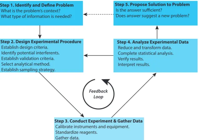
are as many descriptions of the analytical approach as there are analytical chemists, it is convenient to define it as the five-step process shown in Figure 1.3.
Three general features of this approach deserve our attention. First, in steps 1 and 5 analytical chemists have the opportunity to collaborate with individuals outside the realm of analytical chemistry. In fact, many prob-lems on which analytical chemists work originate in other fields. Second, the heart of the analytical approach is a feedback loop (steps 2, 3, and 4) in which the result of one step requires that we reevaluate the other steps. Finally, the solution to one problem often suggests a new problem.
Analytical chemistry begins with a problem, examples of which include evaluating the amount of dust and soil ingested by children as an indica-tor of environmental exposure to particulate based pollutants, resolving contradictory evidence regarding the toxicity of perfluoro polymers during combustion, and developing rapid and sensitive detectors for chemical and biological weapons. At this point the analytical approach involves a collabo-ration between the analytical chemist and the individual or agency working on the problem. Together they determine what information is needed and clarify how the problem relates to broader research goals or policy issues, both essential to the design of an appropriate experimental procedure.
To design the experimental procedure the analytical chemist considers criteria, such as the required accuracy, precision, sensitivity, and detection 7 For different viewpoints on the analytical approach see (a) Beilby, A. L. J. Chem. Educ. 1970, 47, 237-238; (b) Lucchesi, C. A. Am. Lab. 1980, October, 112-119; (c) Atkinson, G. F. J. Chem.
Educ. 1982, 59, 201-202; (d) Pardue, H. L.; Woo, J. J. Chem. Educ. 1984, 61, 409-412; (e)
Guarnieri, M. J. Chem. Educ. 1988, 65, 201-203, (f) Strobel, H. A. Am. Lab. 1990, October, 17-24.
These examples are taken from a series of articles, entitled the “Analytical Ap-proach,” which for many years was a regular feature of the journal Analytical
Chemistry.
To an analytical chemist, the process of making a useful measurement is critical; if the measurement is not of central impor-tance to the work, then it is not analytical chemistry.
An editorial in Analytical Chemistry en-titled “Some Words about Categories of Manuscripts” highlights nicely what makes a research endeavour relevant to modern analytical chemistry. The full ci-tation is Murray, R. W. Anal. Chem. 2008,
80, 4775; for a more recent editorial, see
“The Scope of Analytical Chemistry” by Sweedler, J. V. et. al. Anal. Chem. 2015,
87, 6425.
Chapter 3 introduces you to the language of analytical chemistry. You will find terms such accuracy, precision, and sensitivity defined there.
limit, the urgency with which results are needed, the cost of a single analysis, the number of samples to analyze, and the amount of sample available for analysis. Finding an appropriate balance between these criteria frequently is complicated by their interdependence. For example, improving precision may require a larger amount of sample than is available. Consideration also is given to how to collect, store, and prepare samples, and to whether chemical or physical interferences will affect the analysis. Finally a good experimental procedure may yield useless information if there is no method for validating the results.
The most visible part of the analytical approach occurs in the labora-tory. As part of the validation process, appropriate chemical and physical standards are used to calibrate equipment and to standardize reagents.
The data collected during the experiment are then analyzed. Frequently the data first is reduced or transformed to a more readily analyzable form and then a statistical treatment of the data is used to evaluate accuracy and precision, and to validate the procedure. Results are compared to the origi-nal design criteria and the experimental design is reconsidered, additioorigi-nal trials are run, or a solution to the problem is proposed. When a solution is proposed, the results are subject to an external evaluation that may result in a new problem and the beginning of a new cycle.
See Chapter 7 for a discussion of how to collect, store, and prepare samples for analysis.
See Chapter 14 for a discussion about how to validate an analytical method. Calibra-tion and standardizaCalibra-tion methods, includ-ing a discussion of linear regression, are covered in Chapter 5.
Figure 1 .3 Flow diagram showing one view of the analytical approach to solving problems (modified
after Atkinson.7c
Step 1. Identify and Define Problem
What is the problem’s context? What type of information is needed?
Step 5. Propose Solution to Problem
Is the answer sufficient?
Does answer suggest a new problem?
Step 2. Design Experimental Procedure
Establish design criteria. Identify potential interferents. Establish validation criteria. Select analytical method. Establish sampling strategy.
Step 4. Analyze Experimental Data
Reduce and transform data. Complete statistical analysis. Verify results.
Interpret results.
Step 3. Conduct Experiment & Gather Data
Calibrate instruments and equipment. Standardize reagents.
Gather data.
Feedback Loop
Chapter 4 introduces the statistical analy-sis of data.
Use this link to access the article’s abstract from the journal’s web site. If your institu-tion has an on-line subscripinstitu-tion you also will be able to download a PDF version of the article.
As noted earlier some scientists question whether the analytical ap-proach is unique to analytical chemistry.Here, again, it helps to distinguish between a chemical analysis and analytical chemistry. For an analytically-oriented scientist, such as a physical organic chemist or a public health officer, the primary emphasis is how the analysis supports larger research goals that involve fundamental studies of chemical or physical processes, or that improve access to medical care. The essence of analytical chemistry, however, is in developing new tools for solving problems, and in defining the type and quality of information available to other scientists.
1C Common Analytical Problems
Many problems in analytical chemistry begin with the need to identify what is present in a sample. This is the scope of a qualitative analysis, examples of which include identifying the products of a chemical reaction,
Practice Exercise 1.1
As an exercise, let’s adapt our model of the analytical approach to the development of a simple, inexpensive, portable device for completing bioassays in the field. Before continuing, locate and read the article
“Simple Telemedicine for Developing Regions: Camera Phones and Paper-Based Microfluidic Devices for Real-Time, Off-Site Diagnosis” by Andres W. Martinez, Scott T. Phillips, Emanuel Carriho, Samuel W. Thomas III, Hayat Sindi, and George M. Whitesides. You will find it on pages 3699-3707 in Volume 80 of the journal Analytical Chemistry, which was published in 2008. As you read the article, pay particular attention to how it emulates the analytical approach and consider the following questions:
What is the analytical problem and why is it important?
What criteria did the authors consider in designing their experiments? What is the basic experimental procedure?
What interferences were considered and how did they overcome them? How did the authors calibrate the assay?
How did the authors validate their experimental method? Is there evidence that steps 2, 3, and 4 are repeated?
Was there a successful conclusion to the analytical problem?
Don’t let the technical details in the paper overwhelm you; if you skim over these you will find the paper both well-written and accessible. Click here to review your answers to these questions.
This exercise provides you with an op-portunity to think about the analytical approach in the context of a real analyti-cal problem. Practice exercises such as this provide you with a variety of challenges ranging from simple review problems to more open-ended exercises. You will find answers to practice exercises at the end of each chapter.
screening an athlete’s urine for a performance-enhancing drug, or deter-mining the spatial distribution of Pb on the surface of an airborne par-ticulate. An early challenge for analytical chemists was developing simple chemical tests to identify inorganic ions and organic functional groups. The classical laboratory courses in inorganic and organic qualitative analysis, still taught at some schools, are based on this work.8 Modern methods for
qualitative analysis rely on instrumental techniques, such as infrared (IR) spectroscopy, nuclear magnetic resonance (NMR) spectroscopy, and mass spectrometry (MS). Because these qualitative applications are covered ade-quately elsewhere in the undergraduate curriculum, they receive no further consideration in this text.
Perhaps the most common analytical problem is a quantitative analy-sis, examples of which include the elemental analysis of a newly synthesized compound, measuring the concentration of glucose in blood, or determin-ing the difference between the bulk and the surface concentrations of Cr in steel. Much of the analytical work in clinical, pharmaceutical, environ-mental, and industrial labs involves developing new quantitative methods to detect trace amounts of chemical species in complex samples. Most of the examples in this text are of quantitative analyses.
Another important area of analytical chemistry, which receives some attention in this text, are methods for characterizing physical and chemi-cal properties. The determination of chemichemi-cal structure, of equilibrium constants, of particle size, and of surface structure are examples of a char-acterization analysis.
The purpose of a qualitative, a quantitative, or a characterization analy-sis is to solve a problem associated with a particular sample. The purpose of a fundamental analysis, on the other hand, is to improve our standing of the theory that supports an analytical method and to under-stand better an analytical method’s limitations.
1D Key Terms
characterization analysis fundamental analysis qualitative analysis quantitative analysis
1E Chapter Summary
Analytical chemists work to improve the ability of chemists and other sci-entists to make meaningful measurements. The need to work with smaller samples, with more complex materials, with processes occurring on shorter time scales, and with species present at lower concentrations challenges 8 See, for example, the following laboratory texts: (a) Sorum, C. H.; Lagowski, J. J. Introduction
to Semimicro Qualitative Analysis, 5th Ed.; Prentice-Hall: Englewood, NJ, 1977; (b) Shriner, R.
L.; Fuson, R. C.; Curtin, D. Y. The Systematic Identification of Organic Compounds, 5th Ed.; John Wiley and Sons: New York, 1964.
A good resource for current examples of qualitative, quantitative, characterization, and fundamental analyses is Analytical
Chemistry’s annual review issue that
high-lights fundamental and applied research in analytical chemistry. Examples of re-view articles in the 2015 issue include “Analytical Chemistry in Archaeological Research,” “Recent Developments in Pa-per-Based Microfluidic Devices,” and “Vi-brational Spectroscopy: Recent Develop-ments to Revolutionize Forensic Science.”
analytical chemists to improve existing analytical methods and to develop new ones.
Typical problems on which analytical chemists work include qualitative analyses (What is present?), quantitative analyses (How much is present?), characterization analyses (What are the sample’s chemical and physical properties?), and fundamental analyses (How does this method work and how can it be improved?).
1F Problems
1. For each of the following problems indicate whether its solution re-quires a qualitative analysis, a quantitative analysis, a characterization analysis, and/or a fundamental analysis. More than one type of analysis may be appropriate for some problems.
(a) The residents in a neighborhood near a hazardous-waste disposal site are concerned that it is leaking contaminants into their ground-water.
(b) An art museum is concerned that a recently acquired oil painting is a forgery.
(c) Airport security needs a more reliable method for detecting the presence of explosive materials in luggage.
(d) The structure of a newly discovered virus needs to be determined. (e) A new visual indicator is needed for an acid–base titration.
(f) A new law requires a method for evaluating whether automobiles are emitting too much carbon monoxide.
2. Read the article “When Machine Tastes Coffee: Instrumental Approach to Predict the Sensory Profile of Espresso Coffee,” which discusses work completed at the Nestlé Research Center in Lausanne, Switzerland. You will find the article on pages 1574-1581 in Volume 80 of Analytical
Chemistry, published in 2008. Prepare an essay that summarizes the
nature of the problem and how it was solved. Do not worry about the nitty-gritty details of the mathematical model developed by the authors, which relies on a combination of an analysis of variance (ANOVA), a topic we will consider in Chapter 14, and a principle component regres-sion (PCR), at topic that we will not consider in this text. Instead, focus on the results of the model by examining the visualizations in Figures 3 and 4. As a guide, refer to Figure 1.3 in this chapter for a model of the analytical approach to solving problems.
Use this link to access the article’s abstract from the journal’s web site. If your institu-tion has an on-line subscripinstitu-tion you also will be able to download a PDF version of the article.