Abstract— In this work, computer software that is user-friendly for the analysis and design of brakes was developed. This was done using Microsoft Visual Basic object-oriented programming language. In designing the software, the various classes of brakes were considered. The mathematical expressions that govern the relationship between force, torque, pressure, heat generated rate and energy were assembled and carefully programmed. To enhance the ability to visually display and interpret solutions, graphical features were incorporated in the software. A spectrum of benchmark problems were used to test the software’s robustness, accuracy and efficiency. The results show that the software is highly accurate, efficient and robust. The usage of the software greatly increases the accuracy, and reduces the complexity and time spent in the analysis and design of brakes.
Index Terms — Object-oriented programming, Brake, Torque, Force, Heat generation and dissipation, Computer- aided-design
Notation
contact area, radiating surface area, a1 distance from centre of drum to pivot, m
a3 distance from F2 to shoe pivot (hand brake), m
b1 distance from point of application of force to shoe
pivot, m b2 distance from F1 to the shoe pivot (hand brake), m
C1 constant (external shoe brake)
C2 coefficient of heat transfer, W/m2k
c1 distance from point of application of normal force to
the shoe pivot (external shoe brake ), m c2 moment arm of the actuating force (external shoe
brake), m c3 distance from the point of application of force to the
shoe pivot (hand brake), m Ek total kinetic energy absorbed, W
Ep total potential energy absorbed, W
e natural logarithm base F force applied to the brake shoe, N F1 tension on the right side, N
F2 tension on the slack side
FL force applied to the left block of the brake, N
FR force applied to the right block of the brake
Hb heat generation rate,, W
Mf moment of frictional forces with respect to the shoe
pivot (right shoe), Nm J. A.Akpobi is an Associate Professor with the Department of Production Engineering, Faculty of Engineering, University of Benin, P.M.B 1154, Benin City, Edo State, Nigeria(corresponding author to provide phone: +234 (0) 80 55010348, e-mail: [email protected]).
.
Mf’ moment of frictional force with respect to the shoe pivot,(left shoe), Nm
Mn moment of normal forces with respect to the shoe pivot
( right shoe), Nm Mn’ moment of normal forces with respect to the shoe
pivot,(left shoe), Nm N normal force on the shoe brake, N NL normal force on the left shoe brake,, N
NR normal force on the right shoe brake, N
Pav average pressure, N/m2
Pm maximum pressure (right shoe), N/m2
Pm’ maximum pressure (left shoe), N/m2
R internal radius of drum (external shoe brake), m T torque, Nm V peripheral velocity of drum, m/s ƒ coefficient of friction h distance from center of drum to the pivot, m r internal radius of drum ( internal shoe brake), m w face width of shoe, m α angle of wrap of belt, degrees Δt temperature difference between exposed radiating surface and the surrounding air( degree centigrade or Kelvin) θ angle of contact ( degrees) θ1 center angle from shoe pivot to heel of lining (internal
shoe brake), degrees θ2 center angle from shoe brake to toe of lining (internal
shoe brake), degrees θm center angle from shoe pivot to point of maximum
pressure, degrees
I. INTRODUCTION
The design of brakes involves evaluating the force, pressure, torque, heat-generated, heat dissipated and the coefficient of friction. When in use, the energy absorbed by brakes in the process of slowing down or stop moving part(s)) is dissipated as heat. In the area of brake design, a number of researchers have contributed towards the advancement of the process. One such contribution was from Fazekas; who significantly reduced the difficulty associated with numerical integration in the analysis of circular (Bottom or Puck) pad caliper brake, Fazekas [1]. Ferodo [2] and Neale [3] developed a table for the amount of friction material required for a given average braking power.
In the area of developing software for machine design, very little documented research exists. Some of these documented machine design software include the works of Jombo and Adetona [4]; who worked on belts and pulleys. However, efforts have been made recently to develop software for the design of machine elements, using object-oriented programming technique [5, 6]. Some of these works addressed
Computer-Aided Design Of Brakes
the design of: some types of gears (helical, and spur) see [7, 8], rolling bearings [9], and machine vibrations design [10]. And quite recently, software for the design of Flywheels, was developed and reported, see [11]. Brakes design is well treated in standard machine design texts see refs. [12, 13, 14, 15]. Some commercial software has been developed to design brakes. Most of this software is not robust enough to handle all classes of brakes, while some just consider only electromagnetic brakes, see [16]
The aim of this work is to develop and implement computer software that would greatly facilitate the design of brakes. Consequently in this work we addressed the following engineering design problems [11]: the capability of designing for all brake parameters, reduction of computational complexity and arduous work encountered in brake design, provision of accurate and efficient solutions for brake design process and provision of visual display of program solutions.
II. CLASSIFICATIONOFBRAKES
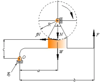
[image:2.595.346.514.100.266.2]There exist many types of brakes and are generally classified as either external, internal or bond brakes. External shoe brakes are further classified into single and double block shoe brakes. External shoe brakes consist of shoes or blocks which are pressed against the rotating surface of the brake drum. Fig. 1 shows a schematic representation of an external single shoe brake. The design of internal shoe brakes largely depends on force, torque, coefficient of friction and the radius of the rotating drum. Fig. 2 shows a schematic representation of an internal shoe brake.
Fig. 1: A schematic representation of an external single shoe brake
.
. Band brakes are flexible bands wrapped partly around
[image:2.595.316.542.339.530.2]the drum. Pulling the band tightly against the drum actuates them. The design of band brakes is dependent on force, angle of wrap, coefficient of friction, pressure on the shoes and radius of the drum. A diagram of a simple two way band brake is shown in fig. 3.
Figure 2: A schematic diagram of internal shoe brake
Fig. 3: A simple two way band brake
III HEAT GENERATED
When the brake is actuated, energy is absorbed, which in turn is dissipated as heat energy. This design is dependent on pressure, area of contact, peripheral velocity, coefficient of friction, potential energy, and kinetic energy, coefficient of heat transfer and area of the radiating surface.
[image:2.595.60.240.430.573.2]A. External Single Shoe Block Brake Design For external single shoe brakes the software was developed using the following:
For a clockwise rotation, the actuating force is given by (1)
1 1
1 (N W a) fNc F
b
+ −
= (1)
The Braking Torque, whenθ ≤ 6 00, is given by (2). When 0
6 0
θ > , the braking torque is given by (3)
T= fNR (2)
, 1 (4 ) 2 ( ) Rsin
T fNh fN
sin θ θ θ ⎛ ⎞ ⎜ ⎟ = = ⎜ + ⎟ ⎜ ⎟ ⎜ ⎟ ⎝ ⎠ (3)
The average pressure is computed using (4): 1 1 2 2 av C sin P
θ
θ
⎛ ⎞ ⎜ ⎟ = ⎜ ⎟ ⎜ ⎟ ⎜ ⎟ ⎝ ⎠ (4) Where 12
(
)
N
C
wR
θ
sin
θ
⎛
⎞
=⎜
+
⎟
⎝
⎠
(5)
B External Double Shoe Block Brake Design For external double shoe brakes the software was developed using (6) – (7)
The braking torque for an external shoe block brake when 0
6 0
θ ≤ , is given by (6) ( L R)
T= f N +N R (6)
Whenθ > 6 00,, the braking torque is computed using (7)
1 (4 ) 2 ( ) ( ) L R Rsin
T fNh f N N
sin θ θ θ ⎛ ⎞ ⎜ ⎟ = = + ⎜ + ⎟ ⎜ ⎟ ⎜ ⎟ ⎝ ⎠ (7)
C Internal Shoe Brake Design The actuating forces are given by (8) – (9)
2
(
n f)
R
M
M
F
c
−
=
(8)
' '
2
(
n f)
L
M
M
F
c
+
=
(9)
Where, and are given by (10) and (11) respectively.
(
)
2 1 1 sin cos sin m f mfp w r
M θ r a d
θ θ θ θ
θ
=
∫
−(10)
2 1 2 1
sin
sin
m n mp wra
M
θd
θ
θ θ
θ
=
∫
(11)
2 m
m
n f
c F p
p
M
M
′ =
+
(12)
'
' n m
n
m
M P
M
P
=
(13)
'
' f m
f
m
M P
M
P
=
(14)
The braking Torque may be determined using (15)
(
)
2 cos 1 cos 2
sin m m
m
T fwr
θ
θ
p pθ
⎛ − ⎞ ′
= ⎜ ⎟ +
⎝ ⎠ (15)
V BAND BRAKE
The force in a Band brake is given as shown in (16)
1 2
f
F
=
F e
α (16) The brake Torque in a band brake is computed using (17)(
1 2)
T
=
F
−
F r
(17) 2 2 1 33
F b F a
F
C
⎛ − ⎞
= ⎜ ⎟
⎝ ⎠ (18)
1 1 f av f F e P wrf e α α α ⎛ − ⎞ = ⎜ ⎟
⎝ ⎠ (19)
VI AMOUNT OF HEAT GENERATED
g av c
H =P A fV
(20)
g k p
H =E +E (21)
g r
H = ΔC tA (22)
g
H = fNV (23)
g av c
H =P A fV (20)
VII PROGRAMME DESCRIPTION
program is structured into three modules as follows: the input stage, the analysis stage and the output stage.
A Input Stage
In this stage, the user provides and enters the basic input parameters of the specific type of brake in the form of data in the respective text boxes of the object interface (form) of the program. The code of the program is written in such a manner that the necessary analyses can be achieved with the entry of minimal number of the basic input parameters.
B Analysis Stage
During this stage, the computer carries out the events initiated by the written code. It processes the data by computing the necessary parameter(s) and stores the result. The result is now ready for the output stage. The speed at which the computer processes the data depends largely on the speed of the microprocessor of the computer.
C Output Stage
This stage involves displaying the processed data numerically as output on the object interface of the program. In this work, the code of the program was written in such a way that the results of the output can be displayed graphically with pre-selected dependent variable versus a pre-selected independent variable.
VIII PROGRAM PSEUDO-CODE ALGORITHM In developing the software the following algorithm or pseudo code was used
Algorithm
If objectsingleshoebrakedesign1.load = true, then Ifθ ≤6 00 then
Enter known parameters: , , , , , N W a b c f ,
Compute the value of the actuating force using equation 1
Else if known input parameters: , , , f N R
θ
Compute the value of torque using equation 2 Beep and note that θ ≤ 6 00
End if End if
If objectsingleshoebrakedesign2.load = true, then If θ > 6 00 then
Enter input parameters: , , ,f N Rθ ,
Compute the value of torque using equation 3 Beep and note that θ >6 00
Else if input parameters are: , , , N R wθ
Compute the value of average pressure, using equation 4
End if End if
If objectdoubleshoebrakedesign.load = true, then Ifθ ≤ 6 00 then
Enter input parameters: , , , f NL NR R,
Compute the value of torque using equation 6
Else ifθ > 6 00then
Enter input parameters: , , , f NL NR R, θ,
Compute the value of torque using equation 7
End if End if
If objectinternalshoebrakedesign.load = true, then
Enter known parameters: Pm, , , , , , , ,f r a w c θ θ θ1 2 m,
Compute the value of the force on the right shoe using equation 8
Compute the value of the force on the left shoe using equation 9
Compute the value of torque using equation 15
End if
If objectbandbrakesdesign.load = true, then If it is simple band brake, then,
If F2 is known, then,
Enter known parameters: F2, e= natural logarithm base, f,
α,
Compute the value of force using equation 16 Else if
F
1 is known, then,Compute the value of force using equation 17 Else if known parameters are:F F1, , 2 r Compute the value of torque using equation 6 End if
Else if it is a differential band brake, then,
Assume a clockwise rotation of drum’
Enter known input parameters: F F1, , , , , , ,2 a b c r w e = natural logarithm base,
Compute the value of force using equation 18
Compute the value of average pressure using equation 19
End if End if
If objectheatgeneratedratedesign.load = true, then, If known input parameters are:Pav, , , Ac f V,
Compute the value of heat generated rate using equation 20
Else if known parameters are , ,Ek Ep
Compute the value of heat generated rate using equation 21
Else if known parameters are: C,Δt, Ar
Compute the value of heat generated rate using equation 22
End if End if
IX NUMERICAL EXAMPLES
To test the efficiency, accuracy and robustness of the software, the following benchmark problems were solved using the software.
EXAMPLE 1
In a given single shoe brake, calculate the force needed to bring the drum to a stop when the normal force is
2083 , N a is 0.36 , m b is 0.9 , m c is0.04m, c is 0.04 , m
coefficient of friction is restricted to be 0.35 and the weight of the brake drum is negligible.
Solution
Fig. 4: Output screen of example 1 EXAMPLE 2
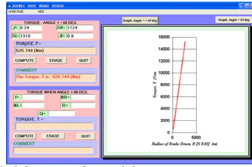
In a double shoe brake, the normal force on the left and the right shoes of a double shoe brake are respectively given as 1310 N and 1124 . N For the given shoe brake, the
coefficient of friction is 0.24 and the internal radius of the drum is 0.9m. Compute the associated torque
.
Solution
[image:5.595.55.297.120.271.2]On entering the specified input parameters, the result was generated as shown in Fig. 5
Fig. 5: Output screen for example 2 EXAMPLE 3
In a differential band brake, the force on the tight side of the band is restricted to be 370N. The internal radius of the drum is
0.16
m
. The angle of wrap is180
0 coefficient of friction0.35, = 0.25 ,a m
= 0.825 0.185b= m and c= m. Compute
the applied force and the generated torque in the brake. Solution
On supplying the specified input parameters, the result was generated as shown in Fig. 6 and Fig.7.
Fig. 6: Output screen for the plot of Applied Force against Angle of wrap in Example 3.
Fig. 7: Output screen for the Plot of Torque vs. Angle of wrap in Example 3
EXAMPLE 4
In a given internal shoe brake, the following parameters were measured: face width of shoe, w = 60mm, coefficient of
friction, f = 0.24, maximum pressure in the right shoe
1.35 / 2, 125
m
P = MN m a= mm, c=225mm, =20 , =135θ1 0 θ2 0
and the radius of the internal drum, r=175mm.
Solution
[image:5.595.308.553.289.437.2] [image:5.595.51.297.441.604.2]Fig. 8: Output screen for Example 4 EXAMPLE 5
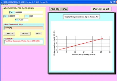
For an experiment carried out on a particular brake, the average working pressure was found to be 1.00 / 2
MN m , the
contact area is 2.4 2
cm , the coefficient of friction is
0.25
andthe associated linear velocity, V =4.325 /m s. Calculate the
power dissipated as heat i.e. (the heat generated rate). Solution
On loading the above parameters in the programmed software, the following result (fig. 9) was produced as output.
Fig. 9: Output screen for Example 5
EXAMPLE 6
In a given brake, the potential energy rate was given as 254.34
p
E = W and the kinetic energy rate was given as
675.23
K
E = W . Calculate the rate of heat generated by the
brake.
Solution
[image:6.595.306.551.121.299.2]On entering the known parameters, the software produced the following results as shown in Fig.10.
Fig. 10 : Output screen for Example 6.
X DISCUSSION OF RESULTS
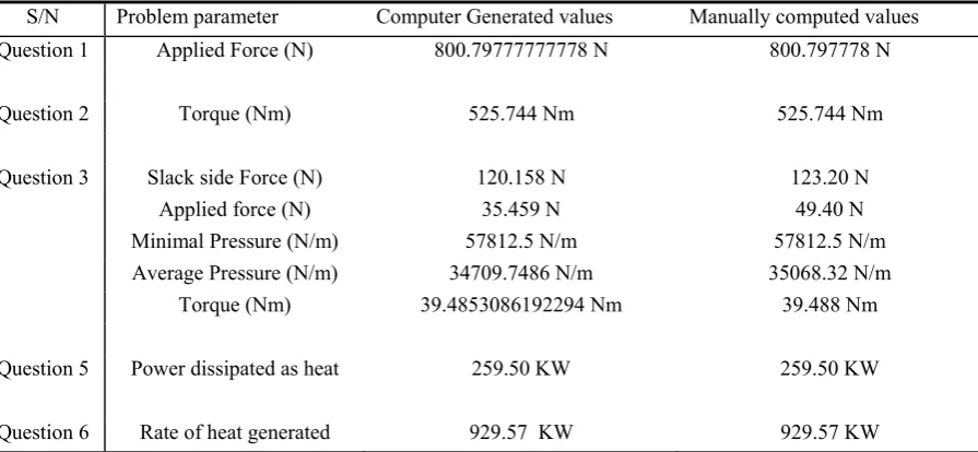
[image:6.595.57.298.423.590.2]Table 1: Software and Manual Results Comparison
S/N Problem parameter Computer Generated values Manually computed values
Question 1 Applied Force (N) 800.79777777778 N 800.797778 N
Question 2 Torque (Nm) 525.744 Nm 525.744 Nm
Question 3 Slack side Force (N) 120.158 N 123.20 N
Applied force (N) 35.459 N 49.40 N
Minimal Pressure (N/m) 57812.5 N/m 57812.5 N/m
Average Pressure (N/m) 34709.7486 N/m 35068.32 N/m
Torque (Nm) 39.4853086192294 Nm 39.488 Nm
Question 5 Power dissipated as heat 259.50 KW 259.50 KW
Question 6 Rate of heat generated 929.57 KW 929.57 KW
Fig. 6 shows that the relationship between the applied force and the angle of wrap of the band of the brake around the brake drum is an inverse curvilinear. Fig. 7 shows that the relationship between the torque and the angle of wrap of the band of the brake around the brake drum is a direct curvilinear. In Fig. 8 as the maximum pressure in the right shoe of the brake increases, the torque generated increases as well, albeit linearly
In Fig. 9 the rate of heat generation displays a direct linear relationship when plotted against the average pressure on the brake. Fig. 10 shows that the rate of heat generation in the brake varies directly and linearly with the rate of kinetic energy dissipation. Table 1 show the comparison between the solution obtained using the developed software and the solution obtained manually. The results are in close agreement.
A Accuracy and Efficiency
To achieve a high precision always for the solutions, we follow the principles adopted in [11]. First we set the design parameters as double precision. This enabled the accuracy of the solutions to be set at 12 decimal places. We eliminated round off errors by using the computation results as obtained in the set 12 decimal format. To enhance the efficiency of the software we incorporated:
1. Highly efficient time management modules 2. Highly efficient memory usage modules
Speed was test for by embedding the complete code for the software in a loop that was made to continue for one hundred times. The program was then executed on a computer with AMD Turion™ 64x2 mobile Technology TL 58 duo core processors with a clock 2GHz and 2MB DDR Ram. When it was executed on this computer it took 28 seconds to provide the solution. This is considerable improvement in speed as compared to manual design approach (about 45 minutes). The efficient memory usage modules contributed to the very fast processing of the solution. The program was designed such
that objects and variables gave up the memory space they occupied at the completion of their assigned tasks.
B Visual Interpretation of Solutions
Graphical features were incorporated in the software to enhance the presentation of the solutions and the ability to speedily and accurately interpret them. Also the graphical solution presents the solution to the specific problem and also extends it. It does this by providing new solutions when a particular parameter is varied (in the design process) while the remaining parameters are held constant. This feature greatly facilitates the teaching of brake design.
C Program Robustness
As stated in [11], a major limitation of commercially available software for machine design is “they provide solutions in a fixed manner”. This is illustrated as follows: A parameter is considered unknown and consequently to be designed for. However when the solution to that design problem is now considered as an unknown parameter and the previously known parameters are treated as unknown, they cannot provide solutions. This problem is easily resolved using the software developed and reported in this work. Thus with this feature we conclude that the developed software is robust to variations in design parameters.
XI CONCLUSION
In this work, computer-aided-design software was developed for brakes. The developed software is basically user-friendly as well as being interactive such that feedback is reported when a wrong entry is entered. Many formulated practical problems have been tested by the software and the results obtained tend to suggest that the software is robust and it also validates the authenticity and accuracy of the software
REFERENCES
[1] G.A. Fazekas, “On circular Spot Brakes”, Trans. ASME, J. Engineering for Industry Series, vol. 94(3), 1972, pp. 859-863.
[2] Ferodo Inc. Friction Materials For Engineers. England: Chapel-en-le- Frith, 1968.
[3] M.I. Neale, The Tribology Handbook. London: Butterworth, 1973.
[4] P.P. Jombo and G.A. Adetona, “Computer-Aided Design of Belts and
Pulley Systems”, Nigerian Journal of Engineering Research and Development, vol. 2(2), 2003, pp. 1-11.
[5] S.G. Byron, Visual Basic, Schaum’s outline series. New Delhi:Tata- McGraw Hill, 2002.
[6] Microsoft Incorporated, Visual Basic 6.0, User’s Guide. Redmond Way: Microsoft Press, 1998.
[7] J.A. Akpobi and J.E. Airiohuodion, “Computer-Aided Design of Helical Gears”, Nigerian Journal of Engineering Research and Development, vol. 8(3), 2007, pp.1-11.
[8] J.A. Akpobi, “Computer Aided Design of Spur Gears”, Technical Transactions of Nigerian Institution of Production Engineers, vol. 4 (1), 1998, pp.110-123.
[9] J.A. Akpobi, “Computer Aided ,Design of Rolling Bearings 1”, Journal of Civil Environmental Systems Engineering, vol. 2(1), 2001, pp.128-141.
[10] J.A. Akpobi and M.Ardey, “ Computer-Aided Design for Machine Vibrations”, Technical Transactions of the Nigerian Institution of Engineers, vol.7(3), 2002, pp. 41-60.
[11] J.A. Akpobi and L.A. Lawani, “Computer Aided Design of Flywheels”, Advances in Engineering Software, vol. 37(4), 2006, pp.222-235,
[12] A.S. Hall, A.R. Holowenko, and H.G. Laughlin, Theory and Problems of Machine Design, Schaum’s outline series, metric edition, London: Tata- McGraw Hill, 2002.
[13] R.S. Khurmi and J.K. Gupta, A Textbook of Machine Design. metric edition, New Delhi: Eurasia Publishing House Limited, 2005.
[14] J.E. Shirgley and C.R. Mischke, Mechanical Engineering Design, 6th Edition, New York : McGraw Hill, 2001.
[15] M.F. Spotts, Design of Machine Elements. 6th Edition, Englewood