Deep BGT at PARSEME Shared Task 2018: Bidirectional LSTM CRF Model for Verbal Multiword Expression Identification

Proceedings of the Joint Workshop on

Linguistic Annotation, Multiword Expressions and Constructions (LAW-MWE-CxG-2018), pages 248–253 Santa Fe, New Mexico, USA, August 25-26, 2018.

248

Deep-BGT at PARSEME Shared Task 2018: Bidirectional LSTM-CRF

Model for Verbal Multiword Expression Identification

G¨ozde Berk, Berna Erden and Tunga G ¨ung¨or

Bo˘gazic¸i University

Department of Computer Engineering 34342 Bebek, Istanbul, Turkey

{gozde.berk, berna.erden, gungort}@boun.edu.tr

Abstract

This paper describes the Deep-BGT system that participated to the PARSEME shared task 2018 on automatic identification of verbal multiword expressions (VMWEs). Our system is language-independent and uses the bidirectional Long Short-Term Memory model with a Conditional Ran-dom Field layer on top (bidirectional LSTM-CRF). To the best of our knowledge, this paper is the first one that employs the bidirectional LSTM-CRF model for VMWE identification. Fur-thermore, the gappy 1-level tagging scheme is used for discontiguity and overlaps. Our system was evaluated on 10 languages in the open track and it was ranked the second in terms of the general ranking metric.

1 Introduction

Baldwin and Kim (2010) define multiword expressions (MWE) as lexical items that have properties that cannot be derived from their component items at the lexical, syntactic, semantic, pragmatic, and/or statistical levels. Moreover, they consider the process of identification of MWEs as the determination of individual occurrences of MWEs in running text.

In this paper, we describe the Deep-BGT system developed for the second edition of the PARSEME shared task on automatic identification of verbal MWEs (VMWE) which covers 20 languages. The corpora provided are in cupt1 format and include annotations of VMWEs consisting of categories de-fined and annotated according to the guidelines provided by Ramisch et al. (2018). The categories of VMWEs are light verb constructions with two subcategories (LVC.full and LVC.cause), verbal idioms (VID), inherently reflexive verbs (IRV), verb-particle constructions with two subcategories (VPC.full and VPC.semi), multi-verb constructions (MVC), inherently adpositional verbs (IAV) and inherently clitic verbs (LS.ICV).

2 Related Work

There are several studies related to identification of multiword expressions. Constant et al. (2017) outline the challenges in the MWE identification task as discontiguity, overlaps, ambiguity, and variability. The flexible nature of these expressions allows reordering or inserting tokens within the MWE components, which results in discontiguity. Discontiguity also poses overlaps such that the gaps in a discontiguous MWE can contain other MWEs. Additionally, it was stated that the MWE identification problem can be addressed using sequence tagging methods with the BIO tagging scheme.

Schneider et al. (2014) describe new tagging schemes that are variants of BIO tagging for MWE iden-tification. One of these, the gappy (discontinuous) 1-level tagging, introduces additional tags to encode gappy MWEs. Huang et al. (2015) propose a bidirectional LSTM-CRF model to solve the sequence tagging problem. While the bidirectional LSTM (Long Short-Term Memory) components consider both the past and future features (Graves et al., 2013), the CRF (Conditional Random Field) component uses

This work is licensed under a Creative Commons Attribution 4.0 International License. License details: http:// creativecommons.org/licenses/by/4.0/

sentence level tag information (Lafferty et al., 2001). Although the bidirectional LSTM-CRF delivers similar performance to stochastic models using external resources in natural language processing bench-mark sequence tagging data sets, its performance does not depend on handcrafted features as in stochastic models. Therefore, the bidirectional LSTM-CRF model is a good option to use as both a non-linear and a statistical approach without relying on hand-crafted features.

Klyueva et al. (2017) implement a supervised approach based on recurrent neural networks to identify VMWEs. The feature set is formed of the concatenation of the embeddings of the tokens surface form, lemma, and POS tag. Legrand and Collobert (2016) present a neural network model that uses the IOBES tagging scheme in order to perform MWE identification.

3 System Description

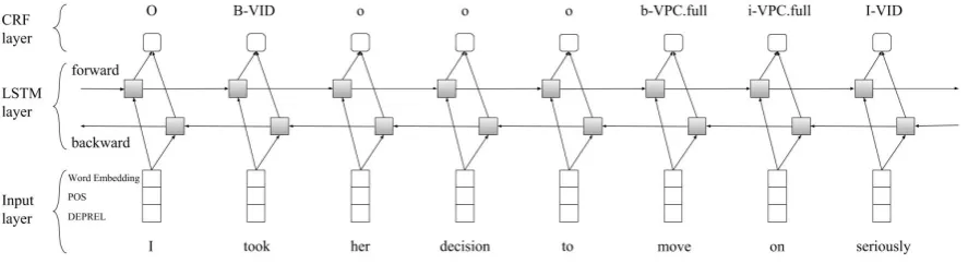
In this paper, we consider the MWE identification task as a sequence tagging problem. We develop a language-independent system based on the bidirectional LSTM-CRF model provided by Huang et al. (2015). In addition, the gappy 1-level tagging scheme is used which was proposed by Schneider et al. (2014). The architecture of the system is shown in Figure 1.

In the training phase, the training set and the development set provided in the cupt format are merged and then preprocessed by applying the tagging format and getting rid of problematic MWEs. Then, the bidirectional LSTM-CRF model runs. In the test phase, the test set is again preprocessed and is executed on the trained model. Afterwards, post processing is applied to convert the output to the cupt format.

Figure 1: Our Bidirectional LSTM-CRF Model.

3.1 Tagging Scheme

For sequence tagging problems, generally the BIO tagging scheme and its variants are used. To overcome the problems of discontiguity and overlaps in MWE identification, the gappy 1-level tagging scheme was proposed by Schneider et al. (2014). In this scheme there are six types of tags, which are B, I, O, b, i, and o. The uppercase tags are similar to the ones in the simple BIO encoding. Bdenotes a token at the beginning of a chunk,Iis used for a token belonging to the remaining part of the chunk, and O

represents a token outside of any chunk. The lowercase labels have similar meanings for gappy chunks.

b corresponds to a token at the beginning of a nested chunk which is within a gap, idenotes a token in the remaining part of the nested chunk, andorepresents a token outside of any chunk within a gap. Since we identify the VMWEs according to their categories in this work, we use the tags B-category, I-category, b-category, i-category(for each category), O, and o. Figure 1 shows two VMWEs, which are ”took seriously” of type VID and ”move on” of type VPC.full.

preserve only one of the MWEs and remove the other MWE(s) during preprocessing. Thus, our model cannot take into account shared MWEs. In fact, the number of such cases is quite limited in the corpora.

3.2 Proposed Model

As shown in Figure 1, the bidirectional LSTM-CRF model consists of three layers. The inputs are word embeddings along with the POS (part-of-speech) and DEPREL (dependency relation) tags provided in the cupt files. Each input vector is represented as a concatenation of the embeddings of word, POS, and DEPREL. We chose the DEPREL tag as a feature in order to capture dependencies at sentence level. We use pre-trained word embeddings released by fastText (Grave et al., 2018), which were trained on Common Crawl and Wikipedia. The vocabulary size of the embeddings is 2M words and the embedding vector dimension is 300.

The input layer passes features to the LSTM layer. The bidirectional LSTM network takes into account both past and future features. On the one side, the forward LSTM units process the sequence from left to right so that they use past information. On the other side, the backward LSTM units process the sequence from right to left so that they use future information. The outputs of the LSTM units are fed into the CRF layer in order to decode the sequence labels. In this way, both non-linear and statistical models are applied to the sequence tagging problem with no extra data engineering.

We use Keras (Chollet and others, 2015) with Tensorflow backend (Abadi et al., 2015) to implement the neural network architecture. Since tuning parameters of the neural network is time intensive, we follow the evaluated network configurations by Reimers and Gurevych (2017). They state that Nadam optimization converges faster than other optimization methods on average after nine epochs, and varia-tional dropout performs better than both naive dropout and no-dropout. They also claim that mini batch sizes between 8 and 32 are good for large training sets, but batch sizes past 64 decrease performance of the network. We chose parameters of the neural network based on these suggestions. Consequently, we apply a fixed dropout rate of 0.1 for all the bidirectional LSTM layers throughout all the experiments. We set batch sizes of 32 for BG, FR, PT, RO and batch sizes of 16 for DE, ES, HU, IT, PL and SL, with regard to the size of the training sets. We trained the model for 12, 15, 15, 12, 15, 12, 12, 12, 12, 12 epochs for, respectively, the languages BG, DE, ES, FR, HU, IT, PL, PT, RO, SL. We set the node size of the network to 20 for each language.

4 Results

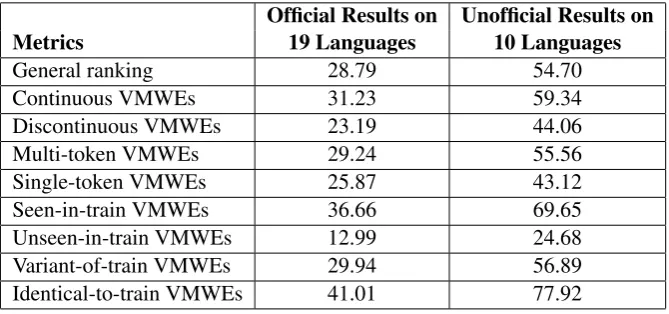
Table 1 shows the cross-lingual macro average results of the Deep-BGT system over 19 languages in the 2018 edition of the PARSEME shared task. The results are given in terms of MWE-based F-measure (F1). Each row in the table represents a metric, including the general metrics and metrics focusing on specific phenomena.

Official Results on Unofficial Results on

Metrics 19 Languages 10 Languages

General ranking 28.79 54.70

Continuous VMWEs 31.23 59.34

Discontinuous VMWEs 23.19 44.06

Multi-token VMWEs 29.24 55.56

Single-token VMWEs 25.87 43.12

Seen-in-train VMWEs 36.66 69.65

Unseen-in-train VMWEs 12.99 24.68

Variant-of-train VMWEs 29.94 56.89

Identical-to-train VMWEs 41.01 77.92

Table 1: The Macro-averaged Results of Deep-BGT.

Table 1) are obtained by averaging the success rates for 19 languages, independent of the number of submitted results. In order to reflect the performance of the Deep-BGT system better, we also show the cross-lingual macro averages over the 10 languages covered (third column in Table 1).

PARSEME shared task allows not only multi-token VMWEs but also single-token ones (abstenersein Spanish,aufmachenin German). Our system can handle single-token VMWEs by means of the gappy 1-level tagging scheme but the performance of the system regarding single-token VMWEs is lower than multi-token ones. The performance of the system for VMWEs unseen in the train data is lower compared to those that occur in both train and test data because it is more troublesome to detect unseen-in-train VMWEs compared to seen-in-train ones. With respect to the variability of the expressions, we see that the success rate for the identical-to-train VMWEs is higher than the variant-of-train VMWEs. Finally, the performance of discontinuous VMWEs is lower than that of continuous VMWEs, as expected.

Five of the languages we covered in the shared task are the Romance languages, which are Spanish (ES), French (FR), Italian (IT), Brazilian Portuguese (PT), and Romanian (RO). We chose the other languages based on two criteria. Since our system learns better with more data, we considered such languages. Also, we favored languages with higher occurring frequency of VMWEs. The frequencies were calculated from the statistics provided along with the corpora. So, we included the languages Bulgarian (BG), German (DE), Hungarian (HU), Polish (PL), and Slovenian (SL) in the experiments. We did not cover Turkish (TR) not to introduce a bias to system evaluation because we were in the Turkish annotation team.

Table 2 gives the results of Deep-BGT for each language separately. MWE-based and Token-based precision (P), recall (R), F-measure (F1), and rankings in the open-track are presented. According to the shared task results, Deep-BGT was ranked first in Bulgarian (BG) in terms of both MWE-based and Token-based F-measure, and was ranked first in German (DE) in terms of MWE-based F-measure. Constant et al. (2017) state that discontiguity is common in Germanic languages. Therefore, the MWE-based results obtained in German adds to the value of BGT. In French (FR) and Polish (PL), Deep-BGT was ranked first regarding the Token-based F-measure. Overall, in general ranking, our system was ranked second among the open-track systems participated in the shared task.

MWE-based Token-based

Languages P R F1 Rank P R F1 Rank

BG 85.96 52.99 65.56 1 91.00 52.82 66.85 1

DE 60.94 36.35 45.53 1 77.92 37.64 50.76 3

ES 24.50 34.20 28.55 2 33.13 38.61 35.66 2

FR 57.81 49.80 53.51 2 78.88 56.45 65.80 1

HU 78.00 71.26 74.48 2 80.71 73.11 76.72 2

IT 45.52 25.60 32.77 2 70.00 27.63 39.62 2

PL 70.87 56.70 63.00 2 80.23 57.85 67.23 1

PT 72.44 46.11 56.35 2 79.40 44.83 57.30 2

RO 79.80 69.10 74.07 2 92.11 73.66 81.86 2

SL 58.90 38.40 46.49 2 72.19 40.34 51.76 2

Table 2: The Language-specific Results of Deep-BGT.

LVC.full LVC.cause VID IRV VPC.full VPC.semi MVC IAV LS.ICV

BG 50.65 26.67 24.14 87.32 - - - 0.00

-DE 4.17 0.00 24.35 33.77 63.47 0.00 - -

-ES 18.03 0.00 6.94 39.22 0.00 - 23.40 31.06

-FR 61.38 0.00 32.26 78.70 - - 0.00 -

-HU 60.00 61.02 62.50 - 74.06 90.24 - -

-IT 31.71 20.51 9.59 51.14 57.89 - 33.33 28.07 0.00

PL 53.72 15.38 3.42 82.40 - - - 61.90

-PT 66.56 0.00 21.94 50.70 - - - -

-RO 68.97 4.65 56.86 85.26 - - - -

-SL 16.33 0.00 10.11 65.61 - - - 44.60

-Table 3: MWE-based F1 scores per VMWE category of Deep-BGT.

LVC.full LVC.cause VID IRV VPC.full VPC.semi MVC IAV LS.ICV

BG 51.45 26.25 31.73 87.53 - - - 0.00

-DE 9.43 0.00 36.62 48.19 67.44 6.25 - -

-ES 21.10 0.00 11.05 39.78 0.00 - 33.50 30.86

-FR 62.67 0.00 59.92 79.35 - - 0.00 -

-HU 65.82 66.07 78.57 - 76.27 89.16 - -

-IT 37.39 26.67 21.13 52.72 58.23 - 30.77 33.85 0.00

PL 55.90 15.69 32.87 83.25 - - - 57.78

-PT 67.60 0.00 28.77 50.35 - - - -

-RO 67.23 75.25 73.45 85.69 - - - -

-SL 21.05 22.22 25.64 66.97 - - - 43.77

-Table 4: Token-based F1 scores per VMWE category of Deep-BGT.

LVC.full LVC.cause VID IRV VPC.full VPC.semi MVC IAV LS.ICV

BG 1635 170 1178 2969 0 0 0 82 0

DE 252 30 1158 268 1485 130 0 0 0

ES 307 53 232 593 0 0 607 447 0

FR 1722 83 1953 1401 0 0 20 0 0

HU 977 373 94 0 4670 870 0 0 0

IT 644 166 1295 1048 83 2 29 458 29

PL 1684 213 430 2030 0 0 0 280 0

PT 3112 87 1012 772 0 0 0 0 0

RO 279 164 1438 3421 0 0 0 0 0

SL 206 52 621 1386 0 0 0 613 0

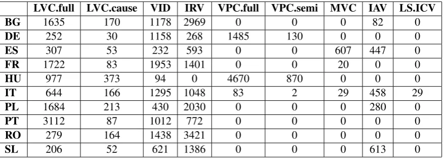
Table 5: Number of VMWEs per VMWE category in the training and the development set.

5 Conclusion

In this paper, we presented the Deep-BGT system that has participated to PARSEME Shared Task Edition 1.1. We followed the sequence tagging approach for VMWE identification. Based on this approach, the gappy 1-level tagging scheme, which is a variant of the BIO scheme, was used. We attempted to solve the discontiguity problem and the nested MWE problem by the proposed model.

Due to the fact that Deep-BGT makes use of deep learning architectures, the more training data is avail-able, the more the system learns. Also, the occurrence frequency of VMWEs in the data plays an impor-tant role. So, results for 10 languages following these criteria were submitted. According to the Shared Task results, the system ranked second in the open track and we conclude that the proposed system obtained successful results.

Acknowledgements

This research was supported by Bo˘gazic¸i University Research Fund Grant Number 14420.

References

Mart´ın Abadi, Ashish Agarwal, Paul Barham, Eugene Brevdo, Zhifeng Chen, Craig Citro, Greg S. Corrado, Andy Davis, Jeffrey Dean, Matthieu Devin, Sanjay Ghemawat, Ian Goodfellow, Andrew Harp, Geoffrey Irving, Michael Isard, Yangqing Jia, Rafal Jozefowicz, Lukasz Kaiser, Manjunath Kudlur, Josh Levenberg, Dande-lion Man´e, Rajat Monga, Sherry Moore, Derek Murray, Chris Olah, Mike Schuster, Jonathon Shlens, Benoit Steiner, Ilya Sutskever, Kunal Talwar, Paul Tucker, Vincent Vanhoucke, Vijay Vasudevan, Fernanda Vi´egas, Oriol Vinyals, Pete Warden, Martin Wattenberg, Martin Wicke, Yuan Yu, and Xiaoqiang Zheng. 2015. Tensor-Flow: Large-Scale Machine Learning on Heterogeneous Systems. Software available from tensorflow.org.

Timothy Baldwin and Su Nam Kim. 2010. Multiword expressions. Handbook of natural language processing, 2:267–292.

Franc¸ois Chollet et al. 2015. Keras.https://keras.io.

Mathieu Constant, G¨uls¸en Eryi˘git, Johanna Monti, Lonneke Van Der 2017. Multiword expression processing: a survey. Computational Linguistics, 43(4):837–892.

Edouard Grave, Piotr Bojanowski, Prakhar Gupta, Armand Joulin, and Tomas Mikolov. 2018. Learning Word Vectors for 157 Languages. InProceedings of the International Conference on Language Resources and

Eval-uation (LREC 2018).

Alex Graves, Abdel-rahman Mohamed, and Geoffrey Hinton. 2013. Speech recognition with deep recurrent neural networks. InAcoustics, speech and signal processing (icassp), 2013 ieee international conference on, pages 6645–6649. IEEE.

Zhiheng Huang, Wei Xu, and Kai Yu. 2015. Bidirectional LSTM-CRF models for sequence tagging. arXiv preprint arXiv:1508.01991.

Natalia Klyueva, Antoine Doucet, and Milan Straka. 2017. Neural Networks for Multi-Word Expression Detec-tion. MWE 2017, page 60.

John Lafferty, Andrew McCallum, and Fernando CN Pereira. 2001. Conditional random fields: Probabilistic models for segmenting and labeling sequence data.

Jo¨el Legrand and Ronan Collobert. 2016. Phrase representations for multiword expressions. InProceedings of

the 12th Workshop on Multiword Expressions, number EPFL-CONF-219842.

Carlos Ramisch, Silvio Ricardo Cordeiro, Agata Savary, Veronika Vincze, Verginica Barbu Mititelu, Archna Bhatia, Maja Buljan, Marie Candito, Polona Gantar, Voula Giouli, Tunga G¨ung¨or, Abdelati Hawwari, Uxoa I˜nurrieta, Jolanta Kovalevskait˙e, Simon Krek, Timm Lichte, Chaya Liebeskind, Johanna Monti, Carla Parra Es-cart´ın, Behrang QasemiZadeh, Renata Ramisch, Nathan Schneider, Ivelina Stoyanova, Ashwini Vaidya, and Abigail Walsh. 2018. Edition 1.1 of the PARSEME Shared Task on Automatic Identification of Verbal Multi-word Expressions. InProceedings of the Joint Workshop on Linguistic Annotation, Multiword Expressions and

Constructions (LAW-MWE-CxG 2018), Santa Fe, New Mexico, USA, August. Association for Computational

Linguistics.

Nils Reimers and Iryna Gurevych. 2017. Reporting score distributions makes a difference: Performance study of lstm-networks for sequence tagging. arXiv preprint arXiv:1707.09861.