Abstract— In the case of multi-echelon and multi-item
inventory systems, the option of accelerated lead time can reduce the inventory cost of the system but on the other hand increase the crashing cost. We utilize an optimization model to show the impact of lead time acceleration by considering component commonality. These imply that lead time is controllable and products taken into example consist of unique and common components. We use some hypothetical data to test the model.
We extend the model for two-echelon inventory system by considering controllable lead time and service level constraint and adding the concept of component commonality in a multi-product’s items case.The results show that most of demand is fulfilled by unique components for both products. Subsequently, the lead time of common component becomes not significant (≈0).
Index Terms— component commonality, accelerated lead time, crashing cost
I. INTRODUCTION
oday’s business is characterized by rapid changes in technology and globalization [1]. The increasing of product variety, product specification, and market demand are some challenges faced by companies in order to realize production efficiency and effectiveness. Production efficiency can be achieved by the attainment of the economic of scale. While, production effectiveness is reflected by the company’s success to deliver the right products for its customers. Supply chain management is viewed as a major solution for cost reduction and productivity [2].
Another impact of technology changes and globalization is product proliferation [1]. Component commonality is one of the most popular supply chain strategies to encounter the challenges of product proliferation such as difficulties in estimating demand, controlling inventory, and providing high customer satisfaction level. It promotes the utilization of common components to replace a number of distinctive parts in various products so that safety stock can be reduced [5].
Manuscript received March 14, 2014; revised April 8, 2014. This work was supported in part by ITB Research and Innovation Grant 2014.
Y. A. Hidayat is with the Research Group on Industrial System and Techno-Economics, Faculty of Industrial Technology, Institut Teknologi Bandung, Ganesa 10, Bandung 40132, Indonesia. (phone: 6222-2504189; email: [email protected]).
Sebrina, M. N. Ardiansyah, and W. J. Sembada were Master students of Industrial Engineering and Engineering Study Program, Faculty of Industrial Technology, Institut Teknologi Bandung Indonesia, Ganesa 10, Bandung 40132, Indonesia (email: [email protected], [email protected], [email protected]).
Previous researches on product proliferation focussed on distinctive parts (DP) and pure component commonality (PCC) strategies. In DP strategy, common component will never be used in all product layers. It is beneficial if the unique components utilization can decrease the material cost. While in PCC strategy, unique components will never be utilized in all layers by replacing a number of distinctive parts in various products so that the safety stock can be reduced. However, both of strategies are not sufficient to produce the optimal solution for the entire supply chain members.
The research on component commonality have been studied by several researchers in [6], [7], and [8]. The objective is to minimize the inventory level and procurement cost caused by the variability of demand. It is assumed that the component lead time is either zero or constant. Binary commonality index by means 0 and 1 or 0 and 100 so that the decision maker can only choose one of the strategies [9].
An empirical study of vertical line extensions from both lower-level end-product and higher-level of end-product is conducted in [10]. The results show that the utilization of commonality can increase the value of the lower-level product and decrease the value of the higher-level end-product. Different quality value of two products is studied in [11]. Later, an inventory model by combining DP and PCC strategies (known as Mixed Component Commonality or MCC) is developed in [4].
This paper is an extention of [4] and [5]. We will investigate the performance of a two-echelon inventory system without and with considering accelerated lead time and by considering the component commonality. Accelerated lead time allows the buyer to accelate the lead time from normal to minimum which will create crashing cost.
II. STUDY DESIGN
The proposed research will investigate the inventory management practices for two-echelon supply chain which consists of single-supplier and single-buyer by considering component commonality. We will use the product structure in Figure 3.1 as our case study. Buyer is assumed as the assembler that produces two type of products i.e. A and B. For producing both products, it can utilize the unique component (a and c) or common component (b). The common component can be used for both products but usually it is more expensive [6].
Integrated Model of Two-Echelon Inventory
System Considering Lead Time Acceleration
and Component Commonality
Y. A. Hidayat, Sebrina, M.N. Ardiansyah, and W. J. Sembada
Based on Figure 1, product A can use unique component a or common component b. While product B, can utilize unique component c or common component b.
A B
b
c a
Final Product
Component
Fig.
1
Product structureThis research considers the following assumptions:
The supply chain sytem in this study consists of single-supplier and single-buyer.
The product structure is multi items which consist of unique or common components.
Demand is probabilistic with normal distribution. The order quantity is constant with lead time L.
Therefore, order will be performed when it reaches the reorder point R.
The price of component is constant in the planning horizon.
The desired value of the demand proportion that is not met from stock is determined by the buyer, so the service level .
The production rate is infinite.
The inventory shortage is fulfilled through backordered mechanism.
∑ is the length of lead time with component 1,2,..., k, crashed to the minimum time, then
∑ ∑ , k = 1,2,...,n. Lead time crashing cost per cycle for [ ] is ( )
( ) ∑ ( ).
A. Notations
Index
: Number of end-product being assembled ( )
: Number of component ( )
: Number of unique component (
)
: Number of common component (
)
: Lead time component
: Lead time component with crashing cost
Parameters
: Buyer demand rate for end-product (unit)
: The standard deviation of buyer’s demand for end-product (unit)
: Unit price of component for end product
(Rp/unit)
: Supplier ordering cost of component for end product for every time of order ($/order)
: Buyer ordering cost of component for end product for every time of order ($/order)
: Buyer holding cost of component for end
product per period (Rp/unit)
: Fixed cost of shortage for component for
end product per unit per time ($/period)
: Crashing cost for lead time component k ($)
: Proportion of component j for end-product i that is not met from the stock (%)
: Bank interest rate (%/year)
: Minimum lead time (year)
: Normal lead time (year)
Variables
: Safety stock of component for product (unit)
: Expected inventory shortage of
component for product (unit)
: Total inventory cost for end-product of supply chain (IDR)
: Total inventory cost (IDR)
: Buyer inventory cost for product (IDR)
: Supplier inventory cost for product (IDR)
: Supplier total inventory cost (IDR)
Decision Variables
: Commonality degree, i.e. percentage of unique component of product produced by using common component
: Order quantity of component for
end-product (unit)
: Lead time of component for end-product
(year)
B. Model Formulation
Buyer:
The buyer inventory cost components consist of purchasing cost, ordering cost, holding cost, shortage cost, and crashing cost as referred in (1) to (5). Equations (6) and (7) summarize buyer inventory cost.
Purchasing cost ( )
(1)
Ordering cost ( )
(2)
Holding cost { (
) √ } { √ } (3)
Shortage cost
( ) √
√
(4)
where ( ) ( )
Crashing cost = ( )
∑ ( ) (
) ∑ ( ) (5)
Hence, buyer’s inventory costs are calculated in (6) and (7).
[ ( ) ]
[ ( )
] [ { ( )√ } {
√ }] [
( ) √
√
] ( ) ∑ ( ) (
) ∑ ( ) (6)
∑ [ ( ) ]
[ ( )
] [ {
( )√ } {
√ }] [
( ) √
√
] ( ) ∑ ( ) (
) ∑ ( )
(7) Supplier:
The supplier inventory cost consist only set-up cost as can be seen in (8).
Set-up cost ( )
(8)
Therefore, the inventory costs of supplier can be calculated as in (9) and (10).
( )
(9)
∑ ( )
(10)
Finally, the total inventory cost is expressed in (11) and (12).
[ ( ) ]
[ ( )
] [ { ( )√ }
{ √ }]
[ ( ) √
√ ]
[ ( )
] (
)
∑ ( ) (
) ∑ ( )
(11)
∑ [ ( ) ]
[ ( )
] [ { ( )√ }
{ √ }]
[ ( ) √
√ ]
[ ( )
] (
)
∑ ( ) (
) ∑ ( ) (12)
a. Constraints
1. Constraints related to decison variables.
layer, and the value between them brings MCC. This relationship is expressed by (13).
(13) For every chosen strategy, number of component to be attached to product should be greater than zero (positive) as shown in (14).
(14) 2. Constraints related to balance flows between
component supply and product demand.
The relationship between total procured component and end-product demand is expressed in (15).
∑ ∑ ∑ (15) The relationship between the total ordered common component and the supported end-products is expressed in (16).
( )
(16) The relationship between the total ordered common component and the supported end-products is expressed in (17).
∑ ∑ ∑ ∑
(17)
b. Solution Techniques
The optimal value of decision variables can be obtained by calculating the partial derivatives of objective function respect to order lot size and lead time. We will explore the solution techniques that are divided into two phases i.e. before and after considering lead time acceleration.
1. Without Lead Time Acceleration
In this phase, the solution will be obtained without considering lead time acceleration so that order will be fulfilled in normal lead time. The solution is acquired with assistance of Lingo version 11.
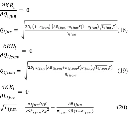
The value of order quantities ( and ) and lead times( and ) are computed by differentiating the buyer inventory cost ( ) as can be seen in (18) to (21).
√
( ) { ( )√ }
(18)
√
{ ( )√ }
(19)
√
( )
(20)
√
(21)
Inserting (20) into (18), we get (22).
( )
(22)
Inserting (21) into (19), we get (23).
(23)
2. With Lead Time Acceleration
In this phase, buyer can speed-up the lead time from normal until minimum. The acceleration will cause additional cost that is called crashing cost. Before buyer accelerates the lead time, the normal lead time must be calculated. In this paper, the value of normal leadtime is acquired from first phase (model without lead time acceleration). Based on the value of normal lead time, we can obtain the other decision variables. The solution technique follows the algoritm below:
1. Determine the value of normal lead time ( ) and minimum lead time ( ) from non-lead time acceleration model for every end-product i and component j.
2. Calculate the value of lead time component by
utilizing ∑
∑ ∑ , k = 1,2,...,m;
; and for normal lead time component ( ) and minimum lead time component( ).
3. Create combination of lead time components. 4. Accelerate the lead time according to the lead
time components so that lead time becomes controllable.
5. Calculate the values of order quantity and commonality degree using (24) and (25).
( )
(24)
(25)
Equation (26) shows the commonality degree.
( )
√
(26)
6. Calculate the total inventory cost ( ). 7. Repeat step four to six for the all combination
of lead time components.
8. The optimal solutions are set of decision variables that produce minimum total cost.
C. Numerical Example
[image:4.595.83.292.578.762.2]TABLE I
THE INITIAL DATA OF NUMERICAL EXAMPLE
Parameter Product A Product B
20,000 10,000 2,000 1,000
20%
j 1 2 2 3
50 52 52 50
1,000 1,200 1,200 1,000 800 1000 1000 800
80 80 80 80
10 10.4 10.4 10
5%
TABLE II
COMPONENT LEAD TIME FOR SUPPLY CHAIN SYSTEM
Normal ( ) (day)
Min ( ) (day)
Unit crashing
cost
Normal ( ) (day)
Min ( ) (day)
Unit crashing
cost
Normal ( ) (day)
Min ( ) (day)
Unit crashing
cost
Normal ( ) (day)
Min ( ) (day)
Unit crashing
cost
119 35 2.8 0 0 2.8 0 0 2.8 91 28 2.8
119 35 8.4 0 0 8.4 0 0 8.4 91 28 8.4
70 49 35 0 0 35 0 0 35 63 35 35
Component Lead Time
(week)
Crashing
Cost Component
Lead Time (week)
Crashing
Cost Component
Lead Time (week)
Crashing
Cost Component
Lead Time (week)
Crashing Cost
0 44 0 0 0 0 0 0 0 0 35 0
1 32 33.6 1 0 0 1 0 0 1 26 25.2
2 20 100.8 2 0 0 2 0 0 2 17 75.6
3 17 105 3 0 0 3 0 0 3 13 140
TABLE III
SOLUTIONS OF MODEL WITHOUT ANDWITHCONSIDERING LEAD TIME ACCELERATION
Decision variables
Optimum value without considering lead time acceleration
Optimum value with considering
lead time acceleration
Units
Cost component
($)
Product A Product B
0.905 0.792 -
Non-Crashing Crashing
Non-Crashing Crashing
0.095 0.209 -
Purchasing cost
1,003,792.55
1,003,793.00
503.792,61
503.792,00
0.190 0.487 -
Ordering cost
5,555.56 5,555.56 5,555.56 5,555.56
0.810 0.513 -
Holding cost
60,684.44
50,199.62 27,564.44
27,530.00
5,995.953 5,995.953 Unit
Shortage cost 27,564.44 17,079.62 11,004.44
10,970.00
603.891 603.891 Unit
Crashing cost -
18,212.28 - -
603.901 603.891 Unit
Buyer’s cost 1,097,597.00
1,094,840.08 547,917.06
547,848.20
2,683.943 2,683.943 Unit
Supplier’s cost 6,787.44 6,787.44 6,787.44 6,787.44
0.852 0.327 Year
Total cost
1,104,384.44
1,101,627.52 554,704.50
554,635.64
0 0 Year
0 0 Year
0.677 0.693 Year
Tabel III shows the comparison of optimal solutions between both stages i.e. with and without lead time acceleration. The computation is done for product A and B. The results show that lead time acceleration will cause reduction on holding cost. The holding cost declines by 17.27% for product A and 0.12% for product B. The same phenomenon also occurs with shortage cost which is 38.04% and 0.31% for product A and B respectively. The cost derivations happen as a trade-off of lead time acceleration that will generate crashing cost. The crashing cost for product A is $ 18,212.28. On the other hand, the crashing cost for product B is zero (no lead time acceleration) because the lead time components for product B are zero.
Lead time acceleration will also cut the total buyer inventory cost even though it initiates the crashing cost. This is due to the fact that the reduction of holding and shortage costs are more significant than the increasing of crashing cost. The decline is about 0.25% and 0.012% for product A and B. Finally, all of cost reductions will reduce the total inventory cost by 0.25% for product A and 0.012% for product B.
III. RESULTS AND DISCUSSION
The optimal solutions are found by calculating all combinatinations of lead time components. It demonstrates the rise on total inventory cost for both models as the crashing cost effect. For both models, the optimal solutions are attained from the same product-component structure. The outputs are shown in a more detail in Table II. It indicates that most of demand is fulfilled by unique components for both products. Subsequently, the lead time of common component becomes not significant (≈0).
IV. CONCLUSION
An optimization model is developed in investigating how the performance of inventory management practices considering the inventory shortage, component commonality degree, and lead time acceleration.
The performance criterion is the total inventory cost. Decision variables are the optimum values of component commonality degree, order quantity and lead time for each component. The constraints are related to decision variables and balance of flows between components supply and products demand. The parameters are unit price of component, supplier’s and buyer’s ordering cost per every
time of order, buyer demand rate, product carrying cost per unit held in buyer’s store in a period, fixed cost of shortage per unit, and cost of shortage per unit per time. The result indicates that most of demand is fulfilled by unique components for both products. Subsequently, the lead time of common component becomes not significant (≈0).
In the future, we will consider the coordination between supplier and buyer in a VMI model. The sensitivity analysis should also be conducted to understand the behavior of model output towards the changing of parameters value.
REFERENCES
[1] H. L. Lee, “Effective inventory and service management through product and process redesign,” Operational Research, vol. 44, no. 1, page 151-156, 1996.
[2] J. Tyan and H. M. Wee, “Vendor managed inventory: a survey of the Taiwanese grocery industry,” Journal of Purchasing and Supply Management, vol. 9, page 11-18, 2003.
[3] S. H. R.Pasandideh, S. T. A.Niaki, A. R. Nia, “An investigation of vendor-managed inventory application in supply chain: the EOQ model with shortage,” International Journal Advanced Manufacturing Technology, vol. 49, page 329-339, 2010.
[4] J. K. Jha and K. Shanker, “Two-echelon supply chain inventory model with controllable lead time and service level constraint,” Computers and Industrial Engineering, vol. 57, page 1096-1104, , 2009.
[5] Y. A. Hidayat, K. Takahashi, K. Morikawa, K. Hamada, L. Diawati, and A.Cakravastia, “Component commonality strategies to achieve mass customization: when a strategy becomes better than the others?,”
ASOR Bulletin, vol. 29, no. 2, page 27-54, 2010.
[6] K. R. Baker, M. J. Magazine, and L. W. Nuttle, “The effect of commonality on safety stock in simple inventory model,” Management Science, vol. 32, page 982-988, 1986.
[7] A. Eynan, “The impact of demand correlation on the effectiveness of component commonality,” International Journal of Production Research, vol. 142, page 523-538, 1996.
[8] Y. Gerchak, M. J. Magazine, and A. B. Gamble, “Component commonality with service level requirement,” Management Science, vol. 34, page 753-760, 1988.
[9] Wazed, M. A., Ahmed, S., and Yusoff, N. 2009. Commonality and its measurement in manufacturing resources planning. Journal of Applied Science, vol. 9, no. 1, page 69-78.
[10]K.Kim and D. Chhajed, “An experimental investigation of valuation change due to commonality in vertical product line extention,” Journal of Product Innovation Management, vol. 18, page 219-230, 2001. [11]H. S.Heese and J. M. Swaminathan, “Product line design with