Experimental study of flow dynamics in close coupled catalyst manifolds

Tim Persoons, 11 May 2006 1 / 34

Experimental study of flow dynamics in close-coupled

catalyst manifolds

Tim Persoons1_{(), Ad Hoefnagels}2 _{and Eric Van den Bulck}1 1 _{Katholieke Universiteit Leuven, dept. Mechanical Engineering}

Celestijnenlaan 300A, B-3001 Leuven, Belgium tel: +32-16-322511, fax: +32-16-322985

email: [email protected]

2 _{BOSAL International, Advanced Engineering and Testing}

Lummen, Belgium

Abstract Time-resolved flow dynamics in an automotive exhaust manifold with

close-coupled catalyst are investigated experimentally on a charged motored engine (CME) flow rig. Flow similarity between CME and fired engine conditions is discussed analytically. Oscillating hot-wire anemometry (OHW) is used to measure the bidirectional phase-locked velocity. Strong time-resolved mean catalyst velocity fluctuations are observed. These are analysed as Helmholtz resonances, using a one-dimensional gas dynamic model of the manifold. The spatial and temporal occurrence of instantaneous reverse flow in the catalyst is investigated, for varying engine load conditions. Periodic backflow occurs throughout large portions of the catalyst cross-section, and proves to be strongly linked to the observed Helmholtz resonances.

Keywords exhaust manifold, close-coupled catalyst, reverse flow, Helmholtz resonance,

oscillating hot-wire anemometry

List of notation

A Cross-sectional area [m2] b Cylinder bore [m]

Cd Discharge coefficient [-], for restricted flow across exhaust valve c Speed of sound [m/s]

cv Specific heat capacity at constant volume [J/kgK] de Diameter of exhaust valve [m]

e, E Index and number of ensembles [-] f Frequency [Hz]

he Lift height of exhaust valve [m]

i, I Index and number of measurement points [-] j, J Index and number of crankshaft positions [-] k Spring constant [N/m]

L Length [m]

Lf Theoretical (stoichiometric) air-to-fuel ratio [-] M Mass flow rate [kg/s]

Ma Mach number [-] m Mass [kg]

Tim Persoons, 11 May 2006 2 / 34 ne Number of exhaust valves per cylinder [-]

p Pressure [Pa]

Q Volumetric flow rate [m3/s]

Re Reynolds number [-], based on runner diameter and mean runner velocity Rf OHW oscillation frequency [-]

r Specific gas constant [J/kgK] Sf Fuel lower heating value [J/kg] s Piston stroke [m]

T Temperature [K] t Time [s] U Velocity [m/s] V Volume [m3]

x, y Measurement coordinates [m] xo OHW oscillation amplitude [m]

Subscripts

0 Top dead centre

1 Peak flow rate during blowdown phase 2 Peak flow rate during displacement phase

a Ambient

bb Blow-by leakage c Combustion cyl Cylinder d Diffuser

e Exhaust, or exhaust valve opening H Helmholtz resonance

i Intake, or intake valve closing m Mean (area-averaged) o OHW (hot-wire oscillator) p Hot-wire probe

r Exhaust runner ref Reference

rel Relative (to hot-wire probe)

s Standard conditions (i.e. 0 °C, 1 atm)

Greek symbols

 OHW tolerance factor [-]

 Exhaust valve opening [rad], in crankshaft angle

Q Flow rate deviation from reference [-]

 Product of equivalence ratio and combustion efficiency [-]

 Flow uniformity measure [-], ratio of mean to maximum velocity

 Ratio of specific heats [-]

 Dynamic viscosity [Pa.s]

 Density [kg/m3_]

 Crankshaft angle [rad]

Tim Persoons, 11 May 2006 3 / 34

1

Introduction

Designing a modern automotive exhaust system requires advanced knowledge on transient fluid dynamics and heat transfer. The exhaust system ‘hot end’ consists of the exhaust manifold with an integrated close-coupled (CC) catalyst. The manifold typically features three to four exhaust runners that converge in a diffuser volume upstream of the catalyst. Downstream of the catalyst, the gas flows through the exit cone and downpipe into the ‘cold end’ of the exhaust system. The CC catalyst is subjected to pulsating flow, alternating between each of the exhaust runners.

The distance between exhaust ports and CC catalyst is preferably as small as possible, to ensure rapid catalyst warm up, thus reducing cold start emissions. However, this requires exhaust runners with small ratios of length and curvature radius to diameter. On the other hand, obtaining high catalyst flow uniformity is crucial for guaranteeing a low pressure drop (and consequently low fuel consumption), high pollutant conversion rate and long catalyst lifetime. Designing such a manifold while ensuring flow uniformity is a formidable task, requiring state-of-the-art knowledge of fluid dynamics and heat transfer in transient internal flows.

Computational Fluid Dynamics (CFD) simulation of such transient three-dimensional flow is difficult using the Reynolds-averaged Navier-Stokes (RANS) approach. The highly curved runners produce strong secondary flows. Separation and recirculation occurs in exhaust runners and diffuser. The flow is characterised by non-isotropic turbulence and three-dimensional boundary layers.

The objective of this research is to provide accurate experimental bidirectional velocity data in the catalyst cross-section, with a high spatial and temporal resolution.

1.1

Flow in close-coupled catalyst manifolds

Persoons et al. [1] discuss previous research by the present authors, using an isothermal flow rig for generating cold pulsating flow in two types of exhaust manifolds. The present paper discusses results obtained on a charged motored engine (CME) flow rig that generates cold pulsating flow, which enables the use of hot-wire anemometry (HWA). Unlike the isothermal flow rig however, the CME flow rig features pulsating exhaust flow with blowdown and displacement phases, typical of fired engine conditions. §2.2 investigates the flow similarity between fired and CME conditions analytically.

Tim Persoons, 11 May 2006 4 / 34

designing a manifold with CC catalyst with respect to the catalyst flow distribution, but that steady state CFD simulations suffice.

Persoons et al. [1, 2] have validated this addition principle for two types of exhaust manifolds; manifolds B and A, with and without exhaust valve overlap. Pulsating flow is generated using two different pulsators; a rotating valve and a motored cylinder head, both mounted on an isothermal flow rig. The flow generated by the isothermal flow rig is quite different from fired engine conditions, although time-averaged Reynolds and Mach number are in accordance.

The findings concerning the addition principle [1, 2] are confirmed to some extent by other sources in literature. Benjamin et al. [3] discuss experimental results on an axisymmetric manifold with catalyst, mounted on an isothermal flow bench with rotating disk pulsator. Traditional phase-locked HWA is used as velocity measurement. No comparison is made between pulsating and stationary flow patterns in terms of the addition principle. Nevertheless, the authors present their results based on the non-dimensional ratio of flow pulsation period to diffuser residence time, similar to the number used in Persoons et al. [1, 2] to characterise the flow and correlate the addition principle’s validity.

Arias-Garcia et al. [4] compare the superposition of stationary velocity distributions with the pulsating flow distribution on a close-coupled catalyst manifold, which is similar to the one used in the present research. The manifold is mounted on an isothermal and motored engine flow rig. The comparison does not hold for the motored engine flow rig.

Liu et al. [5] use the same isothermal flow rig as Benjamin et al. [3], but with more overlapping inlet velocity pulse shapes. Liu et al. [5] report lower catalyst flow uniformity due to overlapping inlet flow pulses when compared to the results of Benjamin et al. [3] featuring non-overlapping pulses. According to Fig. 7 in Liu et al. [5], as the pulsation frequency increases, non-uniformity decreases, i.e. uniformity increases. This is in agreement with our findings. From the same figure, overlapping inlet flow pulses seem to result in a much lower uniformity when compared to non-overlapping pulses. Our research confirms a slightly lower uniformity in the presence of overlap between exhaust valve openings.

Bressler et al. [6] present results obtained using phase-locked laser-Doppler anemometry (LDA) in a four-runner manifold with CC catalyst, mounted on an isothermal flow rig. The authors use a non-dimensional ratio to characterise the flow, similar to Benjamin et al. [3] and Persoons et al. [1].

These and other studies using isothermal pulsating flow rigs do not exhibit reverse flow. This is confirmed by phase-locked LDA results by Hwang et al. [7], obtained on an isothermal flow rig.

1.2

Helmholtz resonances

Tim Persoons, 11 May 2006 5 / 34

and not with the rotating valve as pulsator, most likely because of the different magnitude and frequency content of the excitation exerted by the pulsator to the flow in the manifold. On the CME flow rig, Helmholtz resonances remain present and cause strong catalyst velocity fluctuations. Many sources in literature show similar resonances, although explanations as to their origin vary.

Adam et al. [8] use a one-dimensional gas dynamic model to provide boundary conditions for transient three-dimensional CFD simulation of the flow in a CC catalyst manifold. The simulation results give clear evidence of Helmholtz resonances in fired engine conditions.

Liu et al. [9] combine a one- and three-dimensional model in the same way as Adam et al. [8]. The authors present simulations for a fired and motored engine with atmospheric intake conditions. For fired conditions, simulated runner velocity indicates the presence of strong Helmholtz resonances.

Park et al. [10] present experimental data obtained using phase-locked LDA on a fired engine. The time-resolved runner velocity shows typical fluctuations at frequencies consistent with a Helmholtz resonance.

Benjamin et al. [11] present experimental data obtained using phase-locked LDA on a fired engine. The authors compare their velocity measurements to a numerical approach similar to Liu et al. [9] and Adam et al. [8]. The paper demonstrates fluctuations in runner and catalyst velocity, both in the experimental and numerical data.

Regardless of differences in exhaust system geometries, the findings of the present research are in agreement with those of Adam et al. [8], Liu et al. [9], Park et al. [10] and Benjamin et al. [11]. §3.2 discusses and explains the Helmholtz resonances observed in the current study.

1.3

Reverse flow

Tim Persoons, 11 May 2006 6 / 34

1.4

Measurement techniques

Obtaining high-quality experimental data that captures instantaneous reverse flow is not straightforward. Optical measurement techniques such as LDA are able to measure bidirectional velocity. However, these techniques require high quality optical access and adequate seeding in the entire measurement region. LDA-based research in CC catalyst systems is often plagued with areas of low seeding concentration. This makes it very difficult to obtain a sufficiently high data rate for measuring time-resolved catalyst velocity distributions. Most studies using LDA only measure velocity in a single point or along a single straight line in the manifold.

Hot-wire anemometry (HWA) requires neither optical access nor seeding, although obviously, physical access for the hot-wire probe is required. HWA features a number of advantages including high bandwidth, continuous output signal and good spatial resolution. The main disadvantage of HWA is its inability to discern flow reversal.

A reference work on thermal anemometry by Bruun [13] contains an overview of techniques for measuring in reversing flows using HWA. On one hand, thermal wake probes relate the time-of-flight of a small heated amount of fluid to the local velocity. This approach is characterised by low bandwidth and is better suited for near-wall measurements. On the other hand, flying HWA is used for measuring in free-stream reversing flows. If the hot-wire probe moves at a sufficiently high velocity counter to the normal flow velocity, the relative velocity seen by the probe can remain positive, even though the absolute velocity is negative. Traditional flying HWA devices such as the system described by Thompson and Whitelaw [14] are quite large and cumbersome, making it impossible to use in confined geometries such as exhaust systems.

Persoons et al. [15] describe the calibration of an oscillating hot-wire anemometer (OHW) device, which is used in the current research. The device is calibrated using phase-locked LDA as reference velocity measurement. It is compact enough to be used to measure velocity distributions in the CC catalyst. The OHW features a maximum measurable negative velocity of –1.0 m/s, which is sufficient for the current research. This value is comparable to other flying and oscillating HWA devices.

2

Experimental set up

2.1

CME

Tim Persoons, 11 May 2006 7 / 34

is run without combustion and fuel injection, to obtain cold clean pulsating flow in the exhaust system. The residual cylinder pressure (prior to exhaust valve opening) is adjusted by means of the intake system pressure. By setting the appropriate residual cylinder pressure, the flow in the exhaust system corresponds to various engine load conditions.

T,Z

screw compressor

buffer vessel

pressure regulator

'p pi,ti pcyl

laminar flow meter

pcat

tcat

U

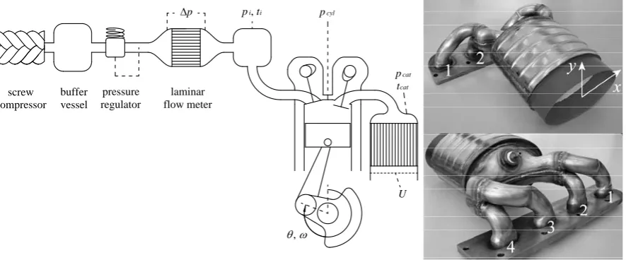
Figure 1. CME flow rig (left) and exhaust manifold (right)

The original exhaust valve timing is unchanged (Table 1). However, the intake camshaft is retarded by 30 °ca to avoid unphysical bthrough from high-pressure intake to low-pressure exhaust system during intake/exhaust valve overlap.

Table 1. Manifold specifications

Engine (valve timing) 1.2l I-4, DOHC 16 valves (+17 | +250 | -220 | +13)1

Runners  28 mm, lengths: (#1) 160 mm, (#2) 80 mm, (#3) 160 mm, (#4) 80 mm Diffuser volume Vd = 390.2 cm3

Catalyst Ceramic 600 cpsi/3 mil, square channels, washcoated. Oval cross-section ( 151 x 101 mm), length 137 mm

The engine is mounted without vibration dampers onto the rigid test stand frame. An automated positioning system is fixed onto the lab floor adjacent to the test stand, taking care to avoid any relative motion between engine exhaust system and velocity probe. The hot-wire oscillator (OHW) is mounted on the positioning system and traversed automatically through the measurement grid.

Figure 1 (left) schematically depicts the CME flow rig. The compressed air is produced using a screw compressor, which delivers a maximum flow rate of 320 kg/h at 8 atm. A pressure regulator maintains a constant pressure in the engine intake system, varying between 1.00 atm to 2.25 atm in the current study. The screw compressor’s maximum flow rate has limited the engine speed in the current measurements to 3000 rpm.

1 _{Valve timing is indicated as IVO | IVC | EVO | EVC. Original intake valve timing has been retarded by 30}

Tim Persoons, 11 May 2006 8 / 34

Intake system flow rate is measured using a laminar flow meter. Partly because of the altered intake timing, intake flow rate is highly pulsating with periods of backflow. Although the laminar flow meter is designed for such flows, the intake system flow rate is further verified using a piezo-electric cylinder pressure sensor. The pressure rise during the compression stroke is used to determine the mass flow rate. The intake flow rate reading is accurate to within 5 % to 10 %, and serves as reference flow rate for the flow rate obtained by integration of the catalyst velocity distribution.

2.2

Flow similarity

The CME flow rig aims to generate pulsating flow in the exhaust manifold that closely resembles fired engine conditions. However, the exhaust flow is cold thus enabling the use of conventional hot-wire anemometry (HWA).

The cold pulsating flow generated by the CME flow rig in the exhaust system is quite different from the isothermal flow rig [1]. By controlling the intake system pressure, the residual cylinder pressure at exhaust valve opening can be adjusted. This results in a two-stage exhaust stroke with blowdown and displacement phases, typical of fired engine conditions.

To compare fired engine conditions with CME and isothermal flow rig conditions, simulations are performed using a filling-and-emptying engine model written in MatlabTM

(e.g. Watson and Janota [17]). The engine model consists of zero-dimensional volumes (intake and exhaust manifold, cylinders) combined with one-dimensional pipes for the intake runners. The model uses the appropriate descriptions for compressible restricted flow over intake and exhaust valves. The combustion process is modelled using a Wiebe law for heat release. Heat loss to the combustion chamber walls is incorporated. Blow-by leakage is taken into account based on experiments on the CME flow rig.

For an engine speed of 1800 rpm and an exhaust flow rate of 100 m3_{/h, Fig. 2 shows the}

time-resolved non-dimensional velocity in runner #1 of manifold B. The solid and dashed lines represent simulations performed for CME and isothermal flow rig. The markers indicate the runner velocity measured on the CME flow rig. The non-dimensional exhaust valve lift is plotted in grey.

Tim Persoons, 11 May 2006 9 / 34

Exhaust valve lift (−)

CME (measured) CME (simulated) ISOT (simulated)

4500 540 630 720

1 2 3 4 5 6 7 8

Crankshaft angle (°)

Runner velocity

U

(r)

(−)

Figure 2. Comparison of exhaust runner velocity for CME and isothermal flow rig [1]

The analytical derivation in the Appendix results in the following expressions for the peak mass flow rate during blowdown M1 [kg/s] and displacement phase M2 [kg/s]:

 

8

1 ₇

1 ₆

3 3 ₆

0

1 2

1

4 1

1 3

0

2 1

1 1

i

e e e i c

i i d

i e i i

ii

i i i c

a a e i i

i i

ii

rT

n d h V T V

M V C

V V T V

p p V T V

p p V T V



 _



 _

 

  

 



 _

 _

 

 _{     }

 

 _{    }  _{  }

 _{   }

   

 

 _{ } 

  _   _    _{ } _{     }  _{ } 

 

 

     _   _

 

 





(1)



1

1 ₁

2

0

2 _{4 2} 1

i c

i

a i i

i

ïi

p T V

b

M s

p T V

 _



 





 _

 

   

  _  _

 _{   }  _{ }

 

    _   _



(2)

In Eqs. (1) and (2), term i represents the influence of the intake system pressure. It varies from

roughly 0.25 to 1 for a fired engine and from 1 to 2.5 for the CME experiments. Term ii

represents the influence of the combustion process, where T_c represents the temperature rise

due to combustion. For the CME flow rig, there is no combustion, reducing term ii to 1.

As the engine load increases, intake system pressure (or equivalently term i) increases. Eqs.

(1) and (2) show that the peak mass flow rate increases during blowdown and decreases during displacement. For the CME flow rig, in the absence of combustion, the intake system pressure should result in peak flow rates comparable to fired engine conditions. An appropriate change in term i should compensate for the change in term ii. Figure 3 shows the

evolution of M1 and M2 according to Eqs. (1) and (2) versus intake pressure, for fired and

CME conditions. M1 and M2 are non-dimensionalised using a reference mass flow rate Mref

Tim Persoons, 11 May 2006 10 / 34

2 ₇₂₀

4 4 180

ref i b M   s 



 

 _{ }

  (3)

Mref corresponds to a hypothetical exhaust stroke of 180 °ca (hence the factor 720/180), where

the total gas mass is exhausted at a constant mass flow rate Mref. For the CME flow rig at low

intake pressure, M1 is negative because of the early opening of the exhaust valve (Vi is smaller

than Ve). This is not the case for the fired engine with original intake valve timing. For the

CME flow rig, the intake camshaft timing is retarded by 30 °ca, to avoid intake/exhaust valve overlap. Valve overlap would yield a high flow rate through the combustion chamber from the high pressure in the intake system to the exhaust system. This does not occur in the fired engine and as such, the intake timing is adjusted on the CME flow rig.

The high ratio of blowdown to displacement peak flow rate M M_{1 2} can only be achieved on

the CME flow rig by increasing intake pressure p pi a to roughly 5. In that case, without altering the compression ratio, the maximum cylinder pressure is too high. Furthermore, because of in-cylinder heat loss, blow-by leakage and the fact that V Vi e1, exhaust flow temperature drops below 0 °C roughly when p p_{i a} 2.5. In that case, water vapour condenses from the air and freezes inside the exhaust manifold. The ice deposits gradually block the small catalyst channels. Possibilities for extending the operating range include using an air heater in the intake system or changing the intake camshaft entirely. None of these options is pursued in this research.

With respect to flow similarity, not only the mass flow rate-based non-dimensional groups

1 ref

M M , M₂ M_ref and M M_{1 2} should be taken into account. The Reynolds and Mach

number based on mean runner velocity and diameter are expressed as:

;

r r r

U d U

Re Ma

rT

  

  ₍₄₎

where Ur = runner mean velocity [m/s] = m





 = dynamic viscosity [Pa.s]. Assuming the exhaust manifold pressure equals atmospheric pressure, the density  can be written as:

1 1

1 0

1

i c

i

a i i

p T V

p T V

 _



 



 _

 

  _    _  _{ }  _{ }

 

Tim Persoons, 11 May 2006 11 / 34

0.4 0.5 0.6 0.7 0.8 0.9 1

−1 0 1 2 3 4 5 6

Fired, 1800 rpm

Mass flow rate (−)

Intake pressure p

i/pa (−)

M

1/Mref (−) (blow−down)

M₂/M_ref (−) (displacement)

M₁/M₂ (−)

1 1.5 2 2.5

−1 0 1 2 3 4 5 6

CME, 1800 rpm

Mass flow rate (−)

Intake pressure p

i/pa (−)

M

1/Mref (−) (blow−down)

M₂/M_ref (−) (displacement)

M₁/M₂ (−)

Figure 3. Mass flow rate2 versus engine load p

i/pa, for (left) fired engine and (right) CME

0.4 0.5 0.6 0.7 0.8 0.9 1

−50 0 50 100 150 200 250

Fired, 1800 rpm

Reynolds number

Re

(10

3)

Intake pressure p

i/pa (−)

Re

1 (10

3

) (blow−down)

Re₂ (103) (displacement)

1 1.5 2 2.5

−50 0 50 100 150 200 250

CME, 1800 rpm

Reynolds number

Re

(10

3)

Intake pressure p

i/pa (−)

Re

1 (10

3

) (blow−down)

Re₂ (103) (displacement)

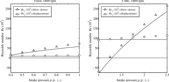
Figure 4. Reynolds number2 _{versus engine load p}

i/pa, for (left) fired engine and (right)

CME

0.4 0.5 0.6 0.7 0.8 0.9 1

−0.1 0 0.1 0.2 0.3 0.4 0.5 0.6

Fired, 1800 rpm

Peak Mach number

Ma

(−)

Intake pressure p

i/pa (−)

Ma

1 (−) (blow−down)

Ma

2 (−) (displacement)

1 1.5 2 2.5

−0.1 0 0.1 0.2 0.3 0.4 0.5 0.6

CME, 1800 rpm

Peak Mach number

Ma

(−)

Intake pressure p

i/pa (−)

Ma

1 (−) (blow−down)

Ma

2 (−) (displacement)

Figure 5. Mach number2 versus engine load p

i/pa, for (left) fired engine and (right) CME

Tim Persoons, 11 May 2006 12 / 34

Due to the strong temperature dependence of the dynamic viscosity, the Reynolds number differs significantly between fired and CME conditions. Figure 4 indicates that the ratio of Re

from CME to fired conditions approximates 2.5 during blowdown and 10 during displacement phase. Figure 5 shows that the Mach number is comparable in CME and fired conditions.

2.3

OHW

To measure bidirectional phase-locked velocity in the exhaust manifold, a hot-wire oscillator (OHW) is used in the current research, which is described in detail in Persoons et al. [15]. The system uses a slider-crank mechanism to oscillate a hot-wire probe with an amplitude xo = 5.5

mm, at a frequency fo from 30 to 40 Hz. A speed-controlled DC motor maintains the

oscillation frequency fo in proportion to the engine speed N [rpm]. The non-dimensional

oscillation frequency Rf is defined as R_f  f_o









probe probe holder oscillating probe holder base

rigid support tube

10 mm

optical encoder

dual balance shafts

speed-controlled DC motor

U > 0

Figure 6. Hot-wire oscillator (OHW) used to measure bidirectional velocity

The normal positive direction of flow is as indicated in Fig. 6. The measured OHW velocity

U is defined as U U_rel U_p, where U_rel = relative velocity as seen by the probe [m/s] and Up = probe velocity [m/s]. The relative velocity U_rel is determined from the anemometer

bridge output voltage, and the probe velocity Up is determined from the oscillator drive shaft

position.

In reverse flow when U 0, the OHW provides a valid measurement as long as the relative

velocity 0U_rel  , or the probe velocity U_p U 0. As the probe oscillates, measurements

are accepted in a window around the maximal negative probe velocity U_p, or symbolically

when Up  2 f xo o   oxo . Approximating the probe motion as purely sinusoidal, this corresponds to arccos  ot2narccos





Tim Persoons, 11 May 2006 13 / 34

When the non-dimensional OHW frequency Rf is a whole number, the OHW moves in

synchronisation with the engine’s crankshaft. In that case, the OHW measurements are taken in the same crankshaft angle intervals in consecutive engine cycles. In order to cover the entire crankshaft position range from 0 to 720 °ca, the OHW motion slightly lags or leads the engine rotation. Rf is arbitrarily chosen as R_f  n 1 4





the choice of  cos





0 180 360 540 720

-1 0 1

-_α

Engine crankshaft position ω t (ο)

Probe velocity

Up

/

ωo

xo

(-)

N = 2400 rpm, f_o = 35.0 Hz, R_f = 1.75

U

p/ωoxo (cycle 1)

U

p/ωoxo (cycle 2)

U

p/ωoxo (cycle 3)

U

p/ωoxo (cycle 4)

U

p = -ωoxoα

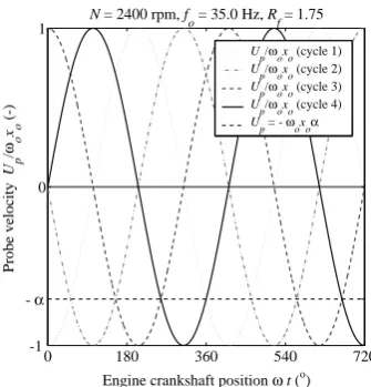
Figure 7. OHW probe velocity, phase-locked with engine crankshaft position

Figure 7 shows the OHW probe velocity versus crankshaft position for a particular engine speed. The oscillator frequency is maximised below 40 Hz, resulting in fo = 35 Hz for N =

2400 rpm, or Rf  2 1 4 1.75 . In this case, it takes four engine cycles to obtain measurements for the entire range of crankshaft position from 0 to 720 °ca. Decreasing the value 1/4 to 1/8 increases the mean probe velocity magnitude during OHW measurements, thus increasing resolution in the negative velocity range. However, instead of four, eight engine cycles would be required to complete measurements for one engine cycle. Obtaining valid measurements for one complete engine cycle (i.e. one ensemble) thus takes four engine cycles. Therefore, several hundred cycles are required to ensure sufficient accuracy after ensemble-averaging the velocity data.

A Dantec StreamLineTM _{HWA system with Dantec type 90C10 constant temperature}

anemometer bridge modules has been used for the current research. A Dantec 55P11 probe with extended prongs is used, as described in Persoons et al. [15]. Calibration of the anemometer bridge output voltage to a reference velocity is performed using a Dantec type 90H02 automated free jet calibrator.

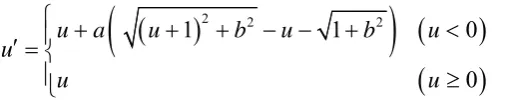
The following non-dimensional correlation is used to convert the OHW velocity reading U

to the actual velocity U. This correlation is obtained during calibration in steady flow, with

negative velocity ranging from U = –1.5 to 0 m/s, and positive velocity ranging from 0 to 10

Tim Persoons, 11 May 2006 14 / 34

















2 _{2 2}

1 1 0

0

u a u b u b u

u

u u

       

   

 _



(6)

where uU oxo, uU oxo, a and b are non-dimensional parameters. a determines the slope





1 o o

uU  x   . In Persoons et al. [15], the values are determined as a0.736 and

0.5

b , with a coefficient of determination R2 0.952.

−4 −3 −2 −1 0

−1 −0.5 0 0.5 1 1.5 2 2.5 3

a = 0.736, b = 0.5 (R2 = 0.952)

OHW velocity

U’

/

ω0

x0

(−)

Reference velocity U/ω

0x0 (−)

10 Hz 20 Hz 30 Hz 40 Hz

Figure 8. Non-dimensional OHW calibration chart at varying oscillation frequency

Figure 8 shows the non-dimensional calibration chart. The solid line represents the correlation fit of Eq. (6). The markers represent measurements at varying oscillation frequency 2₀ between 10 and 40 Hz. The OHW enables the measurement of negative velocity for

1 U _ox_o

  . For an oscillation frequency between 30 and 40 Hz, this corresponds to a maximum measurable negative velocity of roughly –1 m/s. In the positive velocity range, the OHW velocity U equals the reference velocity.

To obtain the catalyst velocity distribution, consecutive measurements are performed in roughly 400 locations in a measurement plane 25 mm downstream of the catalyst outlet face, within a shrouded section to avoid entrainment. Figure 1 (right) shows the coordinate system in the measurement plane that is used for the velocity distribution plots in §3.3. The OHW device is mounted on a Dantec type 41T50 automated positioning system, featuring a positioning accuracy of better than 0.25 mm.

A PC equipped with a dSpaceTM _{DS1103 data acquisition board is used to trigger the velocity}

measurement and control the oscillator frequency fo with the fixed proportionality factor Rf to

Tim Persoons, 11 May 2006 15 / 34

2.4

Data reduction

Ensemble averaging is applied to obtain the phase-locked velocity distributions. As described in §2.3, one ensemble is constructed from data obtained during crankshaft angle windows of valid OHW measurements in several consecutive engine cycles. Valid OHW measurements are possible when the relative velocity Urel seen by the moving hot-wire probe is positive, or

during arccos  ot2narccos





in one particular point









index, j = crankshaft angle index and e = ensemble index. U_{i j e} is converted to U_{i j e} using the

calibration function defined in Eq. (6) and the appropriate parameters a and b.

The resulting ensembles of U_{i j e}





time-resolved velocity U_{i j}













1

1

, , E , , ,

i j i i j i j e i i j e

U x y U x y e

E

 







where E = number of ensembles. Approximately 100 ensembles yield sufficient accuracy on

the time-resolved velocity. More ensembles are needed when compared to the previous measurements on the isothermal flow rig. This is due to cycle-by-cycle variation, a phenomenon typical of internal combustion engine flows. Because of the absence of a combustion process, the CME flow rig is less affected by cyclic variation than a fired engine. Nevertheless, four times more ensembles are required when compared to the isothermal flow rig experiments to obtain an accuracy of 1% on the time-averaged mean velocity.

The time-averaged velocity U_i













1

1

, , ,

J

i i i i j i i j

j

U x y U x y J  





where J = number of crankshaft positions, which is determined by the sampling frequency.

Regardless of engine speed, 256 samples are taken in each engine cycle. For instance at 2400 rpm, this requires a sampling frequency of 5120 Hz. Roughly 2.5 times more samples per engine cycle are taken when compared to previous measurements, due to the presence of blowdown and Helmholtz fluctuations, causing strong transients in the time-resolved velocity.

The mean (or spatial averaged) velocity Um j

 

 









1

1

, , ,

I

m j j i j i i j i i i i

U U x y A x y

A

 



Tim Persoons, 11 May 2006 16 / 34

where I = number of grid points, Ai = cross-sectional area of grid cell i [m2], A = total

cross-sectional area

1

I i i

A







m

U is defined as:

 

1

1 J

m m j j

j

Q U U

J   A





where Q = volumetric flow rate through the catalyst [m3/s]. In all subsequent figures of

velocity distributions, the non-dimensional velocity U [-] is plotted, defined as U U U_m.

The tilde (~) is omitted in the figures.

The flow uniformity measure M [-] is defined as the ratio of mean to maximum velocity. The

absolute value of the velocity is used in the calculation of M. Eq. (11) gives the definitions of

M for a time-averaged and time-resolved velocity distribution:

 

 

 



 



1...

1...

max

max

M m i

i I

M m i

i I U U

U U



   





 

 



 (11)

The flow uniformity M equals unity for an ideally uniform flow distribution (i.e. U_i U_m),

and varies between zero and unity otherwise. Weltens et al. [16] introduced the widely used flow uniformity index W [-] based on the relative variance of the velocity distribution:

1

1 1

2





 



W i m i

i m

U U A

U A (12)

The mean velocity appears in the denominator of Eq. (12), thus the value of  W

 

 

3

Experimental results

3.1

OHW

To assess the effectiveness of the OHW system, a number of engine operating points that feature reverse flow are selected. In these operating points, the oscillator frequency Rf is

increased from zero for a stationary probe to the maximum attainable. As Rf increases, so does

the resolution in the negative velocity range, and consequently the correspondence improves between the exhaust flow rate calculated as the area-averaged OHW velocity distribution and the intake flow rate measured using the laminar flow meter.

Tim Persoons, 11 May 2006 17 / 34

and  are the density of air at standard conditions (0 °C, 1 atm) and exhaust conditions. The intake standard flow rate Qs,in is determined by means of a laminar flow meter in the intake

system. This measurement is further verified using a cylinder pressure sensor, by calculating the cylinder charge per cycle from the pressure rise during the compression stroke. The blow-by leakage standard flow rate Qs,bb is estimated based on a correlation as a function of engine

speed, time-averaged cylinder pressure and temperature. At most, blow-by leakage amounts to 5% of intake flow rate, for full load at low engine speed.

0 1 2 3 4 5 6 7

−0.2 −0.1 0 0.1 0.2 0.3 0.4 0.5 0.6

OHW frequency R_f (−)

Flow rate error

δ

Q

=

Q

/

Qref

− 1 (−)

p

i = 1.0 atm, N = 600 rpm

p

i = 1.0 atm, N = 1200 rpm

p

i = 1.0 atm, N = 1800 rpm

p

i = 1.5 atm, N = 600 rpm

p

i = 1.5 atm, N = 1200 rpm

p_i = 1.5 atm, N = 1800 rpm

p_i = 2.2 atm, N = 1200 rpm

p_i = 2.2 atm, N = 1800 rpm

Exhaust valve lift (−)

0 180 360 540 720

−1 −0.5 0 0.5 1 1.5

N = 600 rpm, p

i = 1 atm, Rf = 0 (dashed) and 6.75 (solid)

Crankshaft angle (°)

Mean velocity (m/s)

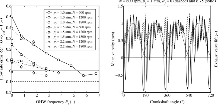
Figure 9. Influence of OHW frequency Rf on flow rate deviation (left) and time-resolved

mean velocity (right)

The markers in Fig. 9 (left) represent experiments at engine speeds of 600, 1200 and 1800 rpm. At low engine load (pi = 1.0 atm), §3.3 demonstrates that strong backflow occurs. This

situation is not physically possible with fired engine conditions. However, local occasional backflow occurs also at higher engine load (pi = 1.5 … 2.2 atm), where positive blowdown

and displacement flows exist.

Figure 9 (left) shows that for increasing OHW oscillation frequency Rf, the velocity

measurement becomes increasingly more accurate. Traditional HWA using a stationary probe corresponds in Fig. 9 (left) to the points at Rf = 0. The flow rate error amounts to anywhere

between 0 and 50%. The OHW approach has reduced the flow rate error to within the accuracy margins on Qref (5 to 10%)

Figure 9 (right) shows the influence of using the OHW on the time-resolved mean velocity

 

m

U  . The dashed line uses a stationary probe (Rf = 0), whereas the solid line uses an

oscillating probe at Rf = 6.75. This experiment corresponds to the rightmost circular marker in

Fig. 9 (left). The mean velocity using traditional HWA (Rf = 0) exhibits the typical

rectification or folding, as HWA is insensitive to the velocity direction, only to its magnitude.

Tim Persoons, 11 May 2006 18 / 34

During those periods, Fig. 9 (right) shows that the OHW velocity at Rf = 0 and Rf = 6.75 yield

identical results.

3.2

Helmholtz resonances

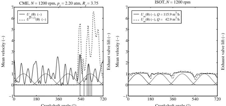
The time-resolved mean velocity U_m

 

previous measurements on an isothermal flow rig [1]. This is due to the two-stage nature of the exhaust stroke, combined with the Helmholtz resonance effect. Figure 10 gives a comparison at equal engine speed and flow rate ( 100 m3_{/h) between the mean velocity on}

the CME (left) and isothermal (right) flow rig. The comparison is presented here since an isothermal flow rig approach is used by numerous authors [1, 3, 5, 6, 7] for studying pulsating flow in exhaust systems with close-coupled catalyst.

Exhaust valve lift (−)

0 180 360 540 720

−1 0 1 2 3 4 5 6 7

CME, N = 1200 rpm, p

i = 2.20 atm, Rf = 3.75

Crankshaft angle (°)

Mean velocity (−)

U_m(θ) (−)

U(r=1)(θ) (−)

Exhaust valve lift (−)

0 180 360 540 720

−1 0 1 2 3 4 5 6 7

ISOT, N = 1200 rpm

Crankshaft angle (°)

Mean velocity (−)

U_m(θ) (−), Q = 115.9 m3/h

U_m(θ) (−), Q = 42.9 m3/h

Figure 10. Time-resolved velocity on CME (left) and isothermal flow rig [1] (right), for

comparable engine speed and flow rate ( 100 m3_/h)

Exhaust valve lift (−)

0 180 360 540 720

−1 0 1 2 3 4 5 6 7

CME, N = 1200 rpm, p

i = 1.55 atm, Rf = 3.75

Crankshaft angle (_°)

Mean velocity (−)

U_m(θ) (−)

U(r=1)(θ) (−)

Exhaust valve lift (−)

0 180 360 540 720

−1 0 1 2 3 4 5 6 7

CME, N = 1200 rpm, p

i = 1.00 atm, Rf = 2.75

Crankshaft angle (_°)

Mean velocity (−)

U

m(θ) (−)

Tim Persoons, 11 May 2006 19 / 34

Figs. 10 (left) and 11 (left) show the time-resolved velocity in runner #1  r 1

 

U   (dashed

line). Since 0 °ca corresponds to top dead centre of cylinder #1 and considering the engine’s firing order, the plots show the exhaust strokes of cylinders #3, #4, #2 and #1. The six vertical lines during the exhaust stroke of cylinder #1 indicate the crankshaft positions (a) through (f) for which the time-resolved velocity distributions are shown in §3.3 (Figs. 17 and 18).

The runner velocity is measured at the inlet of runner #1 using a hot-film sensor, mounted flush with the inner wall.  r 1

U  is measured in a single point, and as such it is only indicative

of the mean runner velocity. It is used to determine the phase lag between runner and catalyst velocity, with respect to the Helmholtz resonance phenomenon.

10 20 50 100 200 500

10−6 10−5 10−4 10−3

Frequency (Hz)

Energy spectral density of

Um

((m/s)

2/Hz)

#3, f

peak = 160.6 Hz

#4, f

peak = 183.1 Hz

#2, f

peak = 181.9 Hz

#1, f_peak = 157.5 Hz

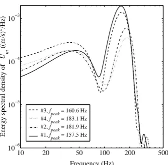
Figure 12. Spectra of time-resolved mean velocity during individual exhaust strokes on CME flow rig, for N = 600 rpm

Table 2. Catalyst mean velocity peak fluctuation frequencies

N pi Qref Peak frequency [Hz] #1 #2 #3 #4 [rpm] [atm] [m3_{/h] [-] [-] [-] [-]}

1200 1.00 46.6 164 181 166 178 1200 1.55 67.7 141 153 126 161 1800 1.00 75.1 148 158 143 144 1200 2.23 93.3 125 173 141 158 1800 1.58 97.4 152 165 141 169 1800 2.23 136.6 143 146 139 144 2400 1.55 192.1 135 193 125 195 2400 2.03 238.8 140 193 153 178 Helmholtz resonance

frequency fH,1 (at 20 °C) 166 188 166 188 Helmholtz resonance

frequency fH,2 (at 20 °C) 182 205 182 205

Tim Persoons, 11 May 2006 20 / 34

fluctuation frequencies observed on CME and isothermal flow rig are identical, varying between 140 and 200 Hz. The frequency is independent of engine speed or flow rate, as the summary in Table 2 shows. The values fH,1and fH,2are discussed below.

Figure 12 shows frequency spectra of Um during each cylinder’s exhaust stroke for N = 600

rpm. As Table 2 indicates, the peak frequency remains unchanged at higher engine speeds. However, the spectral resolution decreases as the engine speed increases, which leads to increasing uncertainty on the peak frequencies.

A Helmholtz resonator consists of a volume connected to a pipe, behaving as a spring-and-mass system. The gas in the pipe behaves as an incompressible plug with spring-and-mass mAL

[kg], where A and L = cross-sectional area [m2] and length [m] of the pipe. The compressible

volume V is characterised by a spring constant k pA V2 [N/m], where  = ratio of

specific heats [-]. This system features an eigenfrequency fH [Hz]:

1 2

H

c AL f

L V



 (13)

where c = speed of sound [m/s]. A Helmholtz resonator is usually a cavity consisting of a

closed volume and a pipe perpendicular to the main flow duct, without net flow through the pipe. Such resonators are used as sound sources in musical instruments, or as acoustic dampers (e.g. in exhaust mufflers). Here, the same resonating behaviour is observed, yet for a system that features net flow. The Helmholtz frequency fH denotes the zeroth order gas

dynamic resonance frequency of the system.

pcyl

Ur U

m kd

kcyl

Vcyl A, L Vd

Figure 13. Lumped model of Helmholtz resonance in CCC exhaust manifold

Up-close examination of the velocity in runner #1 and the catalyst (dashed versus solid lines in Figs. 10 (left) and 11 (left)) reveals that the runner velocity leads the catalyst velocity by

2

 radians. The cylinder pressure is not shown, yet also leads the catalyst velocity by  2

Tim Persoons, 11 May 2006 21 / 34

Since the runners extend into the cylinder head up to the exhaust valves, the lengths in Table 1 are increased by roughly 90 mm. The diffuser volume Vd and cylinder volume Vcyl act as

two compressible springs in series. In terms of Eq. (13), this corresponds to using an effective volume V defined as 1V 1V_d 1V_cyl . The cylinder volume can be approximated by

2 1

0 2 4

cyl

V V  s b corresponding to the mid piston position, where V0 = dead volume, b and

s = cylinder bore and piston stroke.

Using the above effective volume, Eq. (13) yields the values fH,2 in Table 2, slightly

overestimating the resonance frequency. Upon neglecting the diffuser volume compressibility, the effective volume reduces to the cylinder volume, yielding the values fH,1 in Table 2. These

agree better with the experiments, however the assumption that the diffuser volume is incompressible contradicts the observed phase difference between runner and catalyst velocity. This cannot be readily explained, yet might be attributed to the crude approximation of the lumped parameter model.

The exhaust stroke of each individual cylinder features a different resonance frequency, based on each runner’s length. Table 2 gives an overview of measured peak frequencies of the time-resolved mean velocity, for each cylinder’s exhaust stroke and the corresponding Helmholtz eigenfrequencies fH, determined using Eq. (13) as described above.

A one-dimensional gas dynamic model of the exhaust manifold is used to further verify the origin of the mean velocity oscillations. The model is a SimulinkTM _{implementation of a}

second order total variation diminishing (TVD) differencing scheme to simulate unsteady compressible one-dimensional flow in the exhaust runners. The model incorporates the TVD flux differencing technique by Vandevoorde et al. [18]. A grid spacing of 5 mm is applied in each runner. The diffuser is modelled as zero-dimensional compressible volume. The catalyst monolith is modelled as a restriction with coefficients based on pressure drop experiments in steady flow. The inertia of the gas in the monolith is taken into account.

102 103

−60 −50 −40 −30 −20 −10 0

2nd order TVD δx = 5 mm

Magnitude (dB) of

ρ

cU

/pcyl

FRF From: Cylinder pressure p

cyl, To: Catalyst velocity ρcU

Frequency f (Hz)

L = 160 mm (131 Hz) L = 80 mm (181 Hz)

102 103

−60 −50 −40 −30 −20 −10 0

2nd order TVD δx = 5 mm

Magnitude (dB) of

ρ

cU

/pcyl

FRF From: Cylinder pressure p

cyl, To: Catalyst velocity ρcU

Frequency f (Hz)

L = 150 mm (234 Hz) L = 90 mm (274 Hz) L = 120 mm (249 Hz)

Tim Persoons, 11 May 2006 22 / 34

Figure 14 shows numerically determined frequency response functions (FRF) from the cylinder pressure pcyl [Pa] (relative to atmospheric conditions) to the catalyst velocity U [m/s].

The FRF is non-dimensionalised using c [Pa/(m/s)]. Figure 14 shows the FRF of the manifold under investigation (left) and manifold A (right), which has been used in previous experiments [1] and is included here since an improved gas dynamic model is used [1]. Peaks at frequencies above 1 kHz represent acoustic resonances, due to standing wave effects. The Helmholtz resonance frequencies in Fig. 14 (left) are comparable to the frequency fH from Eq.

(13), and to the frequencies in Table 2 observed on the CME flow rig.

Adam et al. [8] present numerical results for a one-dimensional gas dynamic model of a close-coupled catalyst exhaust manifold, mounted on a fired engine. Figure 9 in their paper shows the velocity in each exhaust runner for 3000 rpm at part load. The velocity fluctuations during the displacement phases are very similar to the time-resolved catalyst velocity observed on the CME flow rig. However, fluctuations in their catalyst velocity are much less pronounced compared to the CME flow rig. The fluctuation frequencies during each cylinder’s exhaust stroke differ, depending on the runner length. The estimated fluctuation frequency is 450 Hz for the long runners #1 and #4 and 580 Hz for the short runners #2 and #3. Based on these estimates, the ratio of the length of long to short runners is 1.6, which seems plausible from their paper.

Park et al. [10] present experimental results using LDA for a close-coupled catalyst exhaust manifold, mounted on a fired engine. Figure 5 in their paper shows the velocity in runner #3 for 2000 rpm at part load. Substantial backflow occurs following blowdown, as is observed on the CME flow rig. The estimated fluctuation frequency is 300 Hz. This frequency is too low to be caused by pressure waves as explained by the authors, yet the value corresponds well with a Helmholtz resonance of the manifold.

Liu et al. [9] present numerical results for a close-coupled catalyst manifold in fired engine conditions, obtained using a combined one-dimensional and three-dimensional numerical approach similar to Adam et al. [8]. Figure 7 [9] shows the runner velocity at 3000 rpm and full load. The estimated frequency of the fluctuations during the displacement phase is 310 Hz. Simulation results in Fig. 8 [9] indicate no fluctuations in motored engine conditions. This is unexpected if the Helmholtz resonance assumption stated above is correct. Perhaps the motored and fired cases do not exhibit the same excitation required to invoke the resonance effect. Figure 9 shows numerical and experimental results using LDA, downstream of the catalyst. Reverse flow occurs following blowdown. Although no actual blowdown occurs in motored conditions at atmospheric intake pressure, reverse flow is nonetheless detected in experiments and simulations. For fired conditions, only the simulations show reverse flow.

Tim Persoons, 11 May 2006 23 / 34

dynamics code. Figure 8 in [11] shows a comparison between measured (cross markers) and calculated (solid line) runner velocity. The simulation exhibits significant velocity fluctuations during the displacement phase. The fluctuation frequency is about 375 Hz for the numerical model, which agrees with other fired engine studies [8, 9], whereas the measurement shows a frequency of about 200 Hz.

Eq. (13) shows that the resonance frequency f_H  c T . Since the temperature ratio is

roughly four between fired and CME conditions, the resonance frequency is two times higher (for the same geometry) in fired engine conditions compared to the CME flow rig. This agrees with the observed frequencies in the literature [8, 9, 10], ranging between 300 and 600 Hz.

In conclusion, the velocity fluctuations during the displacement phases observed on the CME flow rig are found in similar exhaust systems in fired engine conditions, both experimentally and numerically.

3.3

Reverse flow

For an engine speed of 1200 rpm and engine load varying between zero, part and full load, Figs. 15 through 18 present time-averaged and time-resolved catalyst velocity distributions measured on the CME flow rig. These representative figures show the spatial and temporal occurrence of reverse flow through the catalyst.

Figure 15 shows on top the time-averaged velocity distributions, and below the corresponding time-resolved mean velocity and flow uniformity according to Eq. (11). Velocity is non-dimensionalised using the time-averaged mean velocity. Velocity distributions are plotted as contour lines, where the corresponding velocity is indicated by the labels and in the vertical velocity scale to the right of each plot. The dashed and dotted contour lines represent unity and zero velocity respectively. Regions of reverse flow below the dotted contour line are shaded. Each velocity distribution plot contains a plot of Uy0 [-], the velocity along the line y

= 0. Figs. 15 and 16 show that the flow uniformity decreases as the engine load increases, or equivalently the flow rate increases.

Figs. 17 and 18 show the evolution of the time-resolved velocity distribution as a function of crankshaft position during the exhaust stroke of cylinder #1, for zero, part and full load. As reference, Fig. 16 shows the catalyst velocity obtained for steady flow through runner #1, at the flow rate corresponding to Figs. 17 and 18.

The crankshaft positions shown in Figs. 17 and 18 correspond to characteristic events during the exhaust stroke of cylinder #1: (a) maximum U_m

 

 

m

U  following blowdown, (c) increasing U_m

 

maximum U_m

 

 

Tim Persoons, 11 May 2006 24 / 34 0 0.5 1 1.5 2 2.5

−75 −50 −25 0 25 50 75

0 1 2 Uy=0 (−) x (mm) −75 −50 −25 0 25 50 75

Time−averaged velocity U (−)

y (mm) 0.8 0.9 0.9 0.9 0.9 0.9 1 1 1 1 1 1 1 1.2 1.2 1.2 1.2 1.2 1.4

N = 1200 rpm, Q ref = 48.9 m

3_{/h (p} i = 1.00 atm)

U

m = 1.177 m/s, ηM = 0.631, ηW = 0.945

0 0.5 1 1.5 2 2.5

−75 −50 −25 0 25 50 75

0 1 2 Uy=0 (−) x (mm) −75 −50 −25 0 25 50 75

Time−averaged velocity U (−)

y (mm) 0.8 0.8 0.8 0.8 0.8 0.9 0.9 0.9 0.9 0.9 0.9 0.9 1 1 1 1 1 1 1 1 1 1 1.2 1.2 1.2 1.2 1.2 1.4 1.4 1.4 1.61.8 N = 1200 rpm, Q

ref = 70.7 m 3_{/h (p}

i = 1.55 atm)

U

m = 1.388 m/s, ηM = 0.536, ηW = 0.923

0 0.5 1 1.5 2 2.5

−75 −50 −25 0 25 50 75

0 1 2 Uy=0 (−) x (mm) −75 −50 −25 0 25 50 75

Time−averaged velocity U (−)

y (mm) 0.7 0.8 0.8 0.8 0.8 0.8 0.8 0.8 0.9 0.9 0.9 0.9 0.9 0.9 0.9 1 1 1 1 1 1 1 1 1.2 1.2 1.2 1.2 1.4 1.4 1.4 1.4 1.6 1.6 1.8 2

N = 1200 rpm, Q ref = 97.2 m

3_{/h (p} i = 2.20 atm)

U

m = 2.356 m/s, ηM = 0.467, ηW = 0.903

Exhaust valve lift (−)

0 180 360 540 720 −1 −0.5 0 0.5 1 1.5 2 2.5

3 CME, N = 1200 rpm, pi = 1.00 atm, Rf = 2.75

Crankshaft angle (°)

Mean velocity, flow uniformity (−)

U_m(θ) (−) η_M(θ) (−)

Exhaust valve lift (−)

0 180 360 540 720 −1 −0.5 0 0.5 1 1.5 2 2.5

3 CME, N = 1200 rpm, pi = 1.55 atm, Rf = 3.75

Crankshaft angle (°)

Mean velocity, flow uniformity (−)

U_m(θ) (−) η_M(θ) (−)

Exhaust valve lift (−)

0 180 360 540 720 −1 −0.5 0 0.5 1 1.5 2 2.5

3 CME, N = 1200 rpm, pi = 2.20 atm, Rf = 3.75

Crankshaft angle (°)

Mean velocity, flow uniformity (−)

U_m(θ) (−) η_M(θ) (−)

Figure 15. Time-averaged catalyst velocity (top) and time-resolved mean catalyst velocity and flow uniformity (bottom) for 1200 rpm at zero (left), part (middle) and full (right) load

−1 0 1 2 3 4 5 6

−75 −50 −25 0 25 50 75

0 2 4 Uy=0 (−) x (mm) −75 −50 −25 0 25 50 75

Stationary velocity U (−)

y (mm) 1 1 1 1 1 1 1 2 2 3 Runner 1, Q

ref = 41.8 m 3_/h

U

m = 1.065 m/s, ηM = 0.331, ηW = 0.875

−1 0 1 2 3 4 5 6

−75 −50 −25 0 25 50 75

0 2 4 Uy=0 (−) x (mm) −75 −50 −25 0 25 50 75

Stationary velocity U (−)

y (mm) 0.5 0.5 1 1 1 1 ₁ 1 1 2 2 3 4

Runner 1, Q ref = 65.4 m

3_/h

U

m = 1.667 m/s, ηM = 0.213, ηW = 0.808

−1 0 1 2 3 4 5 6

−75 −50 −25 0 25 50 75

0 2 4 Uy=0 (−) x (mm) −75 −50 −25 0 25 50 75

Stationary velocity U (−)

y (mm) 0.5 0.5 1 1 1 1 1 1 2 2 3 3 4 5 Runner 1, Q

ref = 93.4 m 3_/h

U

m = 2.379 m/s, ηM = 0.177, ηW = 0.760

Tim Persoons, 11 May 2006 25 / 34 −1 0 1 2 3 4 5 6

−75 −50 −25 0 25 50 75

0 2 4 Uy=0 (−) x (mm) −75 −50 −25 0 25 50 75

Time−resolved velocity U (−)

y (mm) 0.5 0.5 0.5 0.5 1

t = 74.6 ms θ = 537.2 °ca1 3

2 4 N = 1200 rpm, Q

ref = 48.9 m 3_{/h (p}

i = 1.00 atm)

U m(θ)/Um = 0.393

a −1 0 1 2 3 4 5 6

−75 −50 −25 0 25 50 75

0 2 4 Uy=0 (−) x (mm) −75 −50 −25 0 25 50 75

Time−resolved velocity U (−)

y (mm)

0

0

0

t = 76.2 ms θ = 548.4 °ca1 3

2 4 N = 1200 rpm, Q

ref = 48.9 m 3_{/h (p}

i = 1.00 atm)

U

m(θ)/Um = −0.294

b −1 0 1 2 3 4 5 6

−75 −50 −25 0 25 50 75

0 2 4 Uy=0 (−) x (mm) −75 −50 −25 0 25 50 75

Time−resolved velocity U (−)

y (mm) 1 1 1 1 1 1 1 1

t = 77.2 ms θ = 555.6 °ca1 3

2 4

N = 1200 rpm, Q_ref = 48.9 m3/h (p_i = 1.00 atm)

U m(θ)/Um = 1.000

c −1 0 1 2 3 4 5 6

−75 −50 −25 0 25 50 75

0 2 4 Uy=0 (−) x (mm) −75 −50 −25 0 25 50 75

Time−resolved velocity U (−)

y (mm) 2 2 2 2 2 2 2 2 2

t = 73.4 ms θ = 528.8 °ca1 3

2 4 N = 1200 rpm, Q

ref = 70.7 m 3_{/h (p}

i = 1.55 atm)

U m(θ)/Um = 1.920

a −1 0 1 2 3 4 5 6

−75 −50 −25 0 25 50 75

0 2 4 Uy=0 (−) x (mm) −75 −50 −25 0 25 50 75

Time−resolved velocity U (−)

y (mm) −0.5 −0.5 −0.5 −0.5 0

t = 78.5 ms θ = 565.2 °ca1 3

2 4 N = 1200 rpm, Q

ref = 70.7 m 3_{/h (p}

i = 1.55 atm)

U

m(θ)/Um = −0.617

b −1 0 1 2 3 4 5 6

−75 −50 −25 0 25 50 75

0 2 4 Uy=0 (−) x (mm) −75 −50 −25 0 25 50 75

Time−resolved velocity U (−)

y (mm) 1 1 1 1 1 1 1 1 1 1 1

t = 80.4 ms θ = 579.2 °ca1 3

2 4 N = 1200 rpm, Q

ref = 70.7 m 3_{/h (p}

i = 1.55 atm)

U m(θ)/Um = 1.000

c −1 0 1 2 3 4 5 6

−75 −50 −25 0 25 50 75

0 2 4 Uy=0 (−) x (mm) −75 −50 −25 0 25 50 75

Time−resolved velocity U (−)

y (mm) 2 3 3 3 3 3 3 3 3 3

t = 74.0 ms θ = 533.0 °ca1 3

2 4 N = 1200 rpm, Q

ref = 97.2 m 3_{/h (p}

i = 2.20 atm)

U m(θ)/Um = 2.728

a −1 0 1 2 3 4 5 6

−75 −50 −25 0 25 50 75

0 2 4 Uy=0 (−) x (mm) −75 −50 −25 0 25 50 75

Time−resolved velocity U (−)

y (mm) 0.5 0.5 1 1 2 2 3 3 4 4 0 0 0

t = 78.5 ms θ = 565.4 °ca1 3

2 4 N = 1200 rpm, Q

ref = 97.2 m 3_{/h (p}

i = 2.20 atm)

U m(θ)/Um = 0.295

b −1 0 1 2 3 4 5 6

−75 −50 −25 0 25 50 75

0 2 4 Uy=0 (−) x (mm) −75 −50 −25 0 25 50 75

Time−resolved velocity U (−)

y (mm) 0.5 0.5 0.5 0.5 0.5 0.5 1 1 1 1 1 1 1 2 2 2 3 3 4 0

t = 82.0 ms θ = 590.2 °ca1 3

2 4 N = 1200 rpm, Q

ref = 97.2 m 3_{/h (p}

i = 2.20 atm)

U m(θ)/Um = 1.000

c

Tim Persoons, 11 May 2006 26 / 34 −1 0 1 2 3 4 5 6

−75 −50 −25 0 25 50 75

0 2 4 Uy=0 (−) x (mm) −75 −50 −25 0 25 50 75

Time−resolved velocity U (−)

y (mm) 2 2 2 2 2 2 2 2 2 2

t = 78.5 ms θ = 565.2 °ca1 3

2 4

N = 1200 rpm, Q_ref = 48.9 m3/h (p_i = 1.00 atm)

U m(θ)/Um = 2.022

d −1 0 1 2 3 4 5 6

−75 −50 −25 0 25 50 75

0 2 4 Uy=0 (−) x (mm) −75 −50 −25 0 25 50 75

Time−resolved velocity U (−)

y (mm) 1 1 1 1 1 1 1 1 1 1 1 1 1

t = 80.1 ms θ = 576.4 °ca1 3

2 4

N = 1200 rpm, Q_ref = 48.9 m3/h (p_i = 1.00 atm)

U m(θ)/Um = 1.000

e −1 0 1 2 3 4 5 6

−75 −50 −25 0 25 50 75

0 2 4 Uy=0 (−) x (mm) −75 −50 −25 0 25 50 75

Time−resolved velocity U (−)

y (mm) 0 0 0 0

t = 82.0 ms θ = 590.6 °ca1 3

2 4

N = 1200 rpm, Q_ref = 48.9 m3/h (p_i = 1.00 atm)

U

m(θ)/Um = −0.179

f −1 0 1 2 3 4 5 6

−75 −50 −25 0 25 50 75

0 2 4 Uy=0 (−) x (mm) −75 −50 −25 0 25 50 75

Time−resolved velocity U (−)

y (mm) 2 2 2 2 2 2 2 2 2 2

t = 82.0 ms θ = 590.6 °ca1 3

2 4 N = 1200 rpm, Q

ref = 70.7 m 3_{/h (p}

i = 1.55 atm)

U m(θ)/Um = 1.962

d −1 0 1 2 3 4 5 6

−75 −50 −25 0 25 50 75

0 2 4 Uy=0 (−) x (mm) −75 −50 −25 0 25 50 75

Time−resolved velocity U (−)

y (mm) 0.5 0.5 1 1 1 1 1 1 1 1 1 1 1

t = 83.8 ms θ = 603.2 °ca1 3

2 4 N = 1200 rpm, Q

ref = 70.7 m 3_{/h (p}

i = 1.55 atm)

U m(θ)/Um = 1.000

e −1 0 1 2 3 4 5 6

−75 −50 −25 0 25 50 75

0 2 4 Uy=0 (−) x (mm) −75 −50 −25 0 25 50 75

Time−resolved velocity U (−)

y (mm) −0.5 0.5 0.5 0.5 0.5 0.5 0.5 0.5 0.5 0.5 0.5 1 1 1 0 0 0

t = 85.6 ms θ = 616.0 °ca1 3

2 4 N = 1200 rpm, Q

ref = 70.7 m 3_{/h (p}

i = 1.55 atm)

U m(θ)/Um = 0.336

f −1 0 1 2 3 4 5 6

−75 −50 −25 0 25 50 75

0 2 4 Uy=0 (−) x (mm) −75 −50 −25 0 25 50 75

Time−resolved velocity U (−)

y (mm) 2 2 2 2 2 2 2 3 3 4 4

t = 83.6 ms θ = 601.8 °ca1 3

2 4 N = 1200 rpm, Q

ref = 97.2 m 3_{/h (p}

i = 2.20 atm)

U m(θ)/Um = 1.895

d −1 0 1 2 3 4 5 6

−75 −50 −25 0 25 50 75

0 2 4 Uy=0 (−) x (mm) −75 −50 −25 0 25 50 75

Time−resolved velocity U (−)

y (mm) 0.5 1 1 1 1 1 1 1 1 2 2 3

t = 85.3 ms θ = 614.1 °ca1 3

2 4 N = 1200 rpm, Q

ref = 97.2 m 3_{/h (p}

i = 2.20 atm)

U m(θ)/Um = 1.000

e −1 0 1 2 3 4 5 6

−75 −50 −25 0 25 50 75

0 2 4 Uy=0 (−) x (mm) −75 −50 −25 0 25 50 75

Time−resolved velocity U (−)

y (mm) 0.5 0.5 0.5 1 1 0 0 0 0 0 0

t = 87.1 ms θ = 627.2 °ca1 3

2 4 N = 1200 rpm, Q

ref = 97.2 m 3_{/h (p}

i = 2.20 atm)

U m(θ)/Um = 0.295

f

Figure 18. Time-resolved catalyst velocity for 1200 rpm at zero, part and full load (top to bottom), at crankshaft positions d, e, f (left to right)

Tim Persoons, 11 May 2006 27 / 34

During the first part of the blowdown (Fig. 17 (left)), the velocity increases while the flow uniformity remains quite high. The second part of the blowdown (Fig. 17 (centre)) differs according to the engine load. For high engine load, the distribution is characterised by a sharp velocity peak where ru