Munich Personal RePEc Archive
Competitive Bundling
Zhou, Jidong
Yale University
12 December 2015
Online at
https://mpra.ub.uni-muenchen.de/68358/
Competitive Bundling
Jidong Zhou
School of Management
Yale University
December 2015
(First Version: February 2014)
Abstract
This paper proposes a model of competitive bundling with an arbitrary num-ber of …rms. In the regime of pure bundling, we …nd that relative to separate sales pure bundling tends to raise market prices, bene…t …rms, and harm con-sumers when the number of …rms is above a threshold. This is in contrast to the …ndings in the duopoly case on which the existing literature often focuses. Our analysis also sheds new light on how consumer valuation dispersion a¤ects price competition more generally. In the regime of mixed bundling, having more than two …rms raises new challenges in solving the model. We derive the equi-librium pricing conditions and show that when the number of …rms is large, the equilibrium prices have simple approximations and mixed bundling is generally pro-competitive relative to separate sales. Firms’ incentives to bundle are also investigated.
Keywords: bundling, multiproduct pricing, product compatibility, oligopoly
JEL classi…cation: D43, L13, L15
1
Introduction
Bundling is commonplace in many markets. Sometimes …rms only sell packages and no individual products are available for purchase. For example, in the market for CDs,
newspapers, or cable TV (e.g., in the US), …rms do not usually sell songs, articles, or TV channels separately. This is called pure bundling. Other examples include banking accounts, party services, and repair services tied with the product. On the other hand …rms sometimes sell both a package and individual products, but the package is o¤ered at a discounted price relative to the sum of its component prices. Relevant examples include software suites, TV-internet-phone bundles, season tickets, package tours, and value meals. This is calledmixed bundling. In many cases, bundling occurs in markets where …rms compete with each other.
One obvious reason for bundling is economies of scale in production, selling or buying, or complementarity in consumption. For example, traditionally it was too costly to sell newspaper articles separately. There are also other important reasons for bundling. Bundling can be a pro…table price discrimination device to extract more consumer surplus (Stigler, 1968, and Adams and Yellen, 1976).1 Bundling can also be
used as a leverage device by a multiproduct …rm to deter the entry of potential single-product competitors or to induce the exit of existing competitors (Whinston, 1990, and Nalebu¤, 2004).2
The main anti-trust concern about bundling is that it may restrict market compe-tition. One possible reason, as suggested by the leverage theory, is that bundling can lead to foreclosure and so a more concentrated market. Another possible reason is that even for a given market structure, bundling may relax competition and in‡ate market prices because it changes the space of pricing strategies. This is the main research ques-tion in the literature on competitive bundling (see, e.g., Matutes and Regibeau, 1988, and Nalebu¤, 2000, for pure bundling, and Matutes and Regibeau, 1992, Anderson and Leruth, 1993, and Armstrong and Vickers, 2010, for mixed bundling). However the existing research suggests that bundle-against-bundle competition tends to be …ercer than competition with separate sales (or component pricing), and so the second possi-bility of in‡ating market prices is usually not a concern.3 Nevertheless this assessment
of bundling is based on duopoly models.4 In this paper we will argue that considering
1There has been a substantial body of literature which studies bundling as a price discrimination
device. Most papers consider a monopoly market structure. For example, Stigler (1968), Schmalensee (1984) and Fang and Norman (2006) study the pro…tability of pure bundling relative to separate sales, and Adams and Yellen (1976), Long (1984), McAfee, McMillan, and Whinston (1989), and Chen and Riordan (2013) study the pro…tability of mixed bundling. In general bundling can be regarded as a nonlinear pricing scheme (see, e.g., Armstrong, 2015, for a recent survey on this topic).
2See also Choi and Stefanadis (2001), and Carlton and Waldman (2002).
3When a multiproduct …rm competes with a single-product rival, if consumers have heterogenous
valuations for the additional product, bundling can create vertical product di¤erentiation (i.e., the bundlevs a single product) and relax price competition. See Carbajo, de Meza and Seidmann, 1990, and Chen, 1997, for two such examples.
4One exception is Economides (1989). He studies competitive pure bundling when there is an
more …rms can qualitatively change our view of the impact of bundling, especially in the pure bundling case.
There are many markets where more than two …rms compete with each other and adopt bundling strategies.5 The reason why the existing literature on competitive
bundling mainly focuses on the duopoly case is partly because it has not developed a tractable enough model which can be used to study both pure and mixed bundling with an arbitrary number of …rms. This has limited our understanding of how the degree of market concentration might a¤ect …rms’ incentives to bundle and the impact of bundling. This paper aims to …ll this gap in the literature.
The existing works on competitive bundling use spatial models to capture product di¤erentiation,6 and they often use a two-dimensional Hotelling model where consumers
are distributed on a square and two multiproduct …rms are located at two opposite corners. With more than two …rms, however, it becomes less convenient to model product di¤erentiation in a spatial framework. For example, if there are four …rms and each sells three products, it is not obvious what spatial models will be easy to use. In this paper, we will instead adopt a multiproduct version of the random utility framework developed in Perlo¤ and Salop (1985). Speci…cally, a consumer’s valuation for a product is a random draw from some distribution, and its realization is independent across …rms and consumers. This re‡ects, for example, the idea that …rms sell products with di¤erent styles and consumers have idiosyncratic tastes. This framework is ‡exible enough to accommodate any number of …rms and products, and in the case with two …rms and two products it can be converted into a two-dimensional Hotelling model (such that we can compare our results with the existing …ndings from the duopoly model).
Our study of how bundling a¤ects price competition and market performance has broader implications. For example, pure bundling can be regarded as an outcome of product incompatibility. Consider a system (e.g., a computer, a smartphone, a stereo system) that consists of several components (e.g., hardware and software, receiver and speaker). If …rms make their components incompatible with each other (e.g., by not adopting a common standard) or make it very costly to disassemble the system, then consumers have to buy the whole system from a single …rm and cannot mix and match to assemble a new system by themselves.7 Bundling can also arise due to shopping
costs. If consumers need to incur an extra cost to source from more than one store,
5For example, the companies that o¤er the TV-internet-phone service in New York City include at
least Verizon, AT&T, Time Warner, and RCN.
6One exception is Anderson and Leruth (1993). They use a logit model to study competitive mixed
bundling in the duopoly case. Introducing product di¤erentiation is necessary for studying competitive bundling when …rms have similar cost conditions. If there is no product di¤erentiation, prices settle at marginal costs, and so there is no meaningful scope for bundling.
7This is the interpretation adopted in the early works on competitive pure bundling such as Matutes
they have less incentive to multi-stop shop and are more likely to buy all the products they want from a single store. This is like buying the whole package from a single …rm to enjoy a mixed bundling discount. If the extra shopping cost is su¢ciently high, consumers are forced to behave as if they were in the pure bundling situation.
Our study is also relevant to the recent trend of unbundling in many markets (es-pecially in online markets). For example, in the music industry nowadays consumers can download single songs from iTunes or Amazon. A similar idea is emerging in the publishing industry. For instance, Blendle, an online news platform, o¤ers users in Netherlands and Germany access to newspaper and magazine articles on a pay-per-article basis. (A new startup CoinTent is trying to start a similar business in the US market.) In the higher education market, the rapid development of online course plat-forms such as Coursea is creating the possibility of unbundled higher education. Even for non-digital products, unbundling is taking place in some markets where it used to be di¢cult. For example, by using online platforms like Caviar and Served by Stadium, consumers can mix and match their desired dishes from di¤erent restaurants and have them delivered in one order. Unbundling bene…ts consumers in terms of the improved choice ‡exibility, but to evaluate its impact on consumer welfare we also need to un-derstand how unbundling might change market prices. This issue is also related to the recent debate about whether US cable companies should be required to unbundle their TV packages.
In the section on pure bundling, the main message is that the number of …rms can qualitatively matter for the impact of bundling (or unbundling) on prices, pro…ts, and consumer welfare. In the duopoly case we con…rm the existing …ndings (but in a more general setup): compared to separate sales, pure bundling intensi…es price competition and lowers market prices and pro…ts. For consumers this positive price e¤ect often outweighs the loss from the reduced choice ‡exibility caused by bundling. Beyond duopoly, however, we show that under fairly general conditions the opposite is true (i.e., pure bundling raises prices, bene…ts …rms, and harms consumers) when the number of …rms is above a threshold (which can be small). This suggests that even if bundling does not in‡uence market structure, it can be anti-competitive.
of the valuation density. Since bundling yields a thinner tail than separate sales, it leads to fewer marginal consumers and so a less elastic demand. This induces …rms to raise their prices.8 In contrast, when there are relatively few …rms in the market, the
average position of marginal consumers is closer to the mean. Since bundling makes the valuation density more peaked, it leads to more marginal consumers and so a more elastic demand. This induces …rms to reduce their prices.
The existing research on competitive pure bundling argues that bundle-against-bundle competition is more intense than single-product competition because bundling makes a price reduction doubly pro…table. (When a two-product …rm reduces its price, a consumer who switches to it buys both products.) However our analysis suggests that this intuition is incomplete. Essentially it ignores the fact that bundling also changes the number of marginal consumers who will switch due to a price reduction, and this e¤ect tends to work against the double pro…tability e¤ect when there are enough …rms in the market.
In the section on mixed bundling, we …nd that considering more than two …rms raises new challenges in analysis due to the complication of the consumer choice problem. Our main contribution is to propose a method to solve the pricing game with mixed bundling, and to show that under mild conditions the equilibrium prices have simple approximations when the number of …rms is large. For example, when the production cost is zero the bundle discount will be approximately equal to half of the single-product price (i.e., 50% o¤ for the second product). In terms of the impacts of mixed bundling on pro…ts and consumer surplus, they tend to be ambiguous in the duopoly case and depend on the distribution of consumer valuations. However with a large number of …rms mixed bundling bene…ts consumers and harms …rms under mild conditions.
We also study …rms’ incentives to bundle in both parts of the paper. When pure bundling is the only alternative to separate sales (e.g., when bundling is a product compatibility strategy), the number of …rms matters for a …rm’s incentive to bundle. Bundling is the unique Nash equilibrium outcome in duopoly, but when the number of …rms is above some threshold, separate sales can be an equilibrium outcome as well. In some examples separate sales is another equilibrium if and only if consumers pre-fer separate sales to pure bundling. When …rms can choose the more ‡exible mixed bundling strategy, starting from separate sales each …rm has a strict incentive to intro-duce mixed bundling, independent of the number of …rms in the market. That is, when mixed bundling is feasible and costless to implement, separate sales can never be an equilibrium outcome.
Finally, our study of the benchmark case of separate sales also contributes to the
8More precisely, the average position of marginal consumers di¤ers between the two regimes, and
literature on oligopolistic competition. We show that a standard log-concavity condi-tion (which ensures the existence of pure-strategy pricing equilibrium) guarantees that market prices decline with the number of …rms. This result is not new, but we o¤er a simple proof. We also investigate how the dispersion of consumer valuations a¤ects price competition. This provides the foundation for the price comparison result in the pure bundling part, and it is also useful for studying the impact on price competition of any economic activities (such as information disclosure, advertising, and product design) which can change the dispersion of consumer valuations.
The rest of the paper is organized as follows: Section 2 presents the model and Sec-tion 3 analyzes the benchmark case of separate sales. SecSec-tion 4 studies pure bundling, and Section 5 deals with mixed bundling. (A discussion of the related literature will be provided in each section.) We conclude in Section 6, and all omitted proofs and details are presented in the Appendix.
2
The Model
Consider a market where each consumer needs m 2 products. (They can be m
independent products or m components of a system, depending on the interpretation of bundling.) The measure of consumers is normalized to one. There are n 2
…rms, each supplying all the m products. The unit production cost of any product is normalized to zero (so we can regard the price below as the markup). Each product is horizontally di¤erentiated across …rms (e.g., each …rm produces a di¤erent version of the product).9 We adopt the random utility framework in Perlo¤ and Salop (1985) to
model product di¤erentiation. Letxji;k denote the match utility of …rmj’s productifor consumerk. We assume thatxji;k is i.i.d. across consumers, which re‡ects, for instance, idiosyncratic consumer tastes. In the following we suppress the subscriptk. We consider a setting with symmetric …rms and products: xji is distributed according to a common cumulative distribution function (CDF) F with support [x; x] (where x = 1 and
x=1 are allowed), and for a given consumer it is realized independently across …rms and products. Suppose xji has a …nite mean and variance and its density function f is di¤erentiable and bounded. (In Section 4.5.1, we will consider a more general setting where a …rm’s m products can be asymmetric and have correlated match utilities.)10
9It is important to introduce product di¤erentiation at the product level. If di¤erentiation is only
at the …rm level, consumers will one-stop shop even without bundling, which is not realistic in many markets and also makes the study of competitive bundling less interesting.
10In the basic model, for simplicity we have assumed away possible di¤erentiation at the …rm level.
This can be included, for example, by assuming that a consumer’s valuation for …rm j’s productiis uj+xj
i, whereuj is another random variable which is i.i.d. across …rms and consumers but has the
We consider a discrete-choice framework where the incremental utility from having more than one version of a product is zero and so a consumer only wants to buy one version of each product.11 We also assume that a consumer has unit demand for the
desired version of each product. (Elastic demand will be discussed in Section 4.5.2.) If a consumer consumes m products with match utilities (x1; ; xm) (which can be
purchased from di¤erent …rms if …rms are not bundling) and makes a total paymentT, she obtains surplusPmi=1xi T.
If a …rm sells its products separately, it chooses a price vector (pj1; ; pj
m), j =
1; ; n. If a …rm adopts the pure bundling strategy, it chooses a bundle pricePj. In
the …rst part of the paper, we assume that …rms can only take one of the two selling strategies. (This is naturally the case if bundling is a product compatibility strategy or if mixed bundling is too complicated to use.) We will …rst study the regime of separate sales where all …rms sell their products separately. We will then study the regime of pure bundling where all …rms bundle their products, and compare it with the separate sales regime. Finally we will investigate …rms’ incentives to bundle by considering an extended game where each …rm can individually choose whether to bundle its products or not. In the second part of the paper, we allow …rms to use the more general mixed bundling strategy and each …rm needs to specify pricesPj
s for each possible subsets of
its m products. (If m = 2, it can be described by a pair of stand-alone prices ( j1; j2)
together with a joint-purchase discount j.) In all the regimes the timing is that …rms choose their prices simultaneously, and then consumers make their purchase decisions after observing all the prices and match utilities.
As often assumed in the literature on oligopolistic competition, the market is fully covered (i.e., consumers buy all themproducts). This will be the case if consumers do not have outside options, or if on top of the above match utilitiesxji, consumers have a su¢ciently high basic valuation for each product (or if the lower bound of match utility
xis high enough). Alternatively we can consider a situation where the m products are essential components of a system for which consumers have a high basic valuation. In the regimes of separate sales and pure bundling, we will relax this assumption in Section 4.5.2 and argue that the basic insights remain qualitatively unchanged. However, in the regime of mixed bundling this assumption is important for tractability.
11This assumption is made in all the papers on competitive (pure or mixed) bundling. But it is
3
Separate Sales: Revisiting Perlo¤-Salop Model
This section studies the benchmark regime of separate sales. Since …rms compete on each product separately, the market for each product is a Perlo¤-Salop model. Consider the market for product i, and let p be the (symmetric) equilibrium price.12 Suppose
…rmj deviates to pricep0, while other …rms stick to the equilibrium price p. Then the demand for …rmj’s product i is
q(p0) = Pr[xji p0 >max
k6=j fx k
i pg] =
Z x
x
[1 F(x p+p0)]dF(x)n 1 :
(In the following, whenever there is no confusion, we will suppress the integral limits
x and x.) Notice that F(x)n 1 is the CDF of the match utility of the best product i
among then 1competitors. So …rmjis as if competing with one …rm which has match utility distribution F(x)n 1 and charges p. In equilibrium the demand is q(p) = 1=n
since …rms are symmetric to each other.
Firm j’s pro…t from product iis p0q(p0), and in equilibrium it should be maximized atp0 =p. This yields the …rst-order condition forp to be the equilibrium price:
1
p =n
Z
f(x)dF(x)n 1 : (1)
This condition is also su¢cient for de…ning the equilibrium price if f is log-concave (see Caplin and Nalebu¤, 1991).13 In the uniform distribution example withF(x) =x,
it is easy to see that p = 1=n, and in the extreme value distribution example with
F(x) = e e x
(which generates the logit model), one can check that p = n=(n 1). Notice that with full market coverage, shifting the support of the match utility does not a¤ect the equilibrium price.
In the following, we study two comparative static questions which are important for our subsequent analysis.
Price and the number of …rms. The …rst question is: how does the equilibrium price vary with the number of …rms? Let us rewrite (1) as
p= q(p)
jq0(p)j =
1=n
R
f(x)dF(x)n 1 : (2)
The numerator is a …rm’s equilibrium demand and it decreases withn. The denominator is the absolute value of a …rm’s equilibrium demand slope. It measures the density of a
12In the duopoly case Perlo¤ and Salop (1985) have shown that the pricing game has no asymmetric
equilibrium. Beyond duopoly Caplin and Nalebu¤ (1991) show that there is no asymmetric equilibrium in the logit model. More recently Quint (2014) proves a general result (see Lemma 1 there) which implies that our pricing game has no asymmetric equilibrium iff is log-concave.
13Caplin and Nalebu¤ (1991) provide a slightly weaker su¢cient condition which requiresf to be
1
n+1-concave. Our subsequent analysis needs this to be true for any n, and when n ! 1 this
…rm’s marginal consumers who are indi¤erent between its product and the best product among its competitors. How the denominator changes with n depends on the shape of f. For example, if the density f is increasing, it increases with n and so p must decrease withn. Conversely if f is decreasing, it decreases with n, which works against the demand size e¤ect. However, as long as the denominator does not decrease with
n too quickly, the equilibrium price decreases with n. The following result reports a su¢cient condition for that.
Lemma 1 Suppose 1 F is log-concave (which is implied by the log-concavity of f). Then p de…ned in (1) decreases with n. Moreover, limn!1p = 0 if and only if
limx!x 1f(Fx()x) =1.
Proof. Let x(n 1) be the second highest order statistic of fx1; ; xng. Let F(n 1)
and f(n 1) be its CDF and density function, respectively. Using
f(n 1)(x) = n(n 1)(1 F(x))F(x)n 2f(x) ;
we can rewrite (1) as14
1
p =
Z
f(x)
1 F(x)dF(n 1)(x) : (3)
Since x(n 1) increases in n in the sense of …rst order stochastic dominance, p decreases
inn if the hazard ratef =(1 F)is increasing (or equivalently, if 1 F is log-concave). The limit result also follows from (3) becausex(n 1) converges to x asn ! 1.
Anderson, de Palma, and Nesterov (1995) is the …rst paper that proves this monotonic-ity result (see their Proposition 1). Our proof is simpler than theirs. (Their proof requires f to be log-concave, which is slightly stronger than 1 F being log-concave.) More recently, Quint (2014) shows that when f is log-concave, prices are strategic complements and the pricing game is supermodular in a general setting which allows for asymmetric …rms and the existence of an outside option. Then the monotonicity result follows, since introducing an additional …rm is the same as treating that …rm as an existing one which drops its price from in…nity to the equilibrium price level.15
Though less general, our method is simple and also o¤ers a tail behavior condition for the markup to converge to zero in the limit.
14The right-hand side of (3) is the density of all marginal consumers in the market. A consumer is
a marginal one if her best product and second-best product have the same match utility. Conditional onx(n 1)=x, the CDF ofx(n) is
F(z) F(x)
1 F(x) forz x, and so its density function atx(n)=xis the
hazard rate 1f(Fx()x). Integrating this according to the distribution ofx(n 1)yields the right-hand side
of (3). Dividing it byngives the density of each …rm’s marginal consumers (i.e.,jq0
(p)j).
15Weyl and Fabinger (2013) make a similar observation through the lens of pass-through rate: the
Notice that the log-concavity of 1 F is not a necessary condition. Even if 1 F
is not log-concave, it is still possible that price decreases with n.16 But if 1 F is
log-convex (and the equilibrium price is still determined by (1)), then the same proof implies that p increases in n. The tail behavior condition for limn!1p= 0 is satis…ed
if f(x) > 0. But it can be violated if f(x) = 0. For instance, in the extreme value distribution example we mentioned before, the price p = n=(n 1) converges to 1 in the limit.
Price and the dispersion of consumer valuations. The second comparative static question is: if the distribution of consumer valuations becomes less “dispersed” from f
tog as illustrated in Figure 1 below, how will the equilibrium price change? Intuitively, less dispersed consumer valuations mean less product di¤erentiation across …rms, and so this should intensify price competition and induce a lower market price. (This must be the case if the density g degenerates at one point such that all products become homogenous.) However, this intuition is not totally right, and g does not necessarily lead to a lower market price thanf. As we show below, it depends on how to rank the dispersion of two random variables.
0.0 0.2 0.4 0.6 0.8 1.0
0 1 2
f
[image:11.595.185.409.375.534.2]x g
Figure 1: An example of less dispersed consumer valuations
In the literature on stochastic orders there are several possible ways to rank the dispersion of two random variables. (The classic reference on this topic is Chapter 3 in Shaked and Shanthikumar, 2007.) One of them is convex order. It is the most familiar one for economists because it is equivalent to a mean-preserving spread when two random variables have equal means.17 For example, f and g in Figure 1 can be
16One such example is the power distribution: F(x) =xk withk
2(1n;1). In this example,1 F is neither log-concave nor log-convex. But one can check that the equilibrium price isp= nk 1
n(n 1)k2 and it decreases inn.
17Letx
F and xG be two random variables, and let F andGbe their CDFs, respectively. Then xG
ranked in this order if they have equal means.18 However, as we will see below this
order usually does not ensure a clear-cut price comparison result.
Another one isdispersive order. A random variablexG is said to be smaller thanxF
in the dispersive order (denoted asxG disp xF) ifG 1(t) G 1(t0) F 1(t) F 1(t0)
for any 0< t0 t <1, where Gand F are the CDFs ofxG and xF, respectively. (This
means that the di¤erence between any two quantiles ofGis smaller than the di¤erence between the corresponding quantiles of F.) Dispersive order ensures a clear-cut price comparison result as shown in the following result, but we will also see that it is in general a too strong condition for our bundling application.19
Lemma 2 Consider two Perlo¤-Salop markets with consumer valuations denoted byxF
andxG, respectively. LetF andGbe their CDFs,f andgbe their density functions, and
[xF; xF] and [xG; xG] be their supports, respectively. Without loss of generality suppose E[xF] = E[xG]. Let pk, k = F; G, be the equilibrium price associated with xk. Suppose
both f and g are log-concave such that the equilibrium prices are determined as in (1). (i) If xG is less dispersed than xF according to the dispersive order, then pG pF for
anyn 2.
(ii) However, if f(xF)> g(xG), then there exists n^ such that pG > pF for n >n^.
Proof. Changing the integral variable from x tot=F(x), we get
1
pF
=n
Z xF
xF
f(x)dF(x)n 1 =n
Z 1
0
lF(t)dtn 1 ;
where lF(t) f(F 1(t))and tn 1 is a CDF on [0;1]. Similarly, we have
1
pG
=n
Z 1
0
lG(t)dtn 1 ;
where lG(t) g(G 1(t)). Then
pG pF ,
Z 1
0
[lF(t) lG(t)]dtn 1 0 : (4)
(i) xG disp xF if and only if F 1(t) G 1(t) increases in t 2 (0;1). This implies
that
dF 1(t)
dt
dG 1(t)
dt ,lF(t) lG(t) :
function whenever the expectations exist. WhenxF amd xG have equal means, the equivalence to
a mean-preserving spread is established in Theorem 3.A.1. in Shaked and Shanthikumar (2007).
18According to Theorem 3.A.44. in Shaked and Shanthikumar (2007), a su¢cient condition forf to
be a mean-preserving spread ofg when they have equal means is thatf g changes its sign twice in the order+; ;+. (More generally two densities ranked by convex order can cross each other many times.)
19When two random variables have equal means, dispersive order implies convex order. (See Theorem
Therefore,pG pF follows from (4). (In particular,xG disp xF implies lF(1) lG(1),
orf(xF) g(xG).)
(ii)f(xF)> g(xG) implies lF(1) lG(1)>0. Then
lim
n!1
Z 1
0
[lF(t) lG(t)]dtn 1 =lF(1) lG(1)>0;
since lF(t) lG(t) is bounded (given we consider bounded density functions) and the
distribution tn 1 converges to the upper bound 1 as n ! 1. Then it follows from (4)
that pG> pF when n is su¢ciently large.20
Result (i) shows that if one distribution is less dispersed than the other in the dispersive order, the usual intuition works and less dispersed consumer valuations lead to a lower market price. Perlo¤ and Salop (1985) show that ifxG = xF with 2(0;1),
then pG < pF (more precisely, pG = pF). This is a special case of result (i) since x <disp xfor any random variable x and constant 2(0;1). (Here “<disp” denotes a strict dispersive order.)
However, dispersive order is a relatively strong condition. When xF and xG have
the same …nite support,xG disp xF requiresF 1(t) G 1(t)increase int 2(0;1), but
this impliesF 1(t) =G 1(t) everywhere, i.e., the two random variables must be equal.
This excludes many natural cases where one random variable is intuitively less dispersed than the other. For instance, the two distributions in Figure 1 cannot be ranked by the dispersive order. (When xF and xG have equal means and their supports are intervals, xG disp xF requires that the support of xG is a strict subset of the support of xF, or
both are in…nite supports.)
Notice that f(xF) > g(xG) is not compatible with xG disp xF as we already see
from the proof. So result (ii) indicates that if we go beyond the dispersive order, even in natural cases such as the example in Figure 1 where one distribution is intuitively less dispersed than the other, the number of …rms can matter for price comparison. When there are su¢ciently many …rms, a less dispersed distribution can lead to a higher market price. Since this result is crucial for understanding our price comparison result in the pure bundling part, we explain its economic intuition in detail.
Let us consider the example in Figure 1 where f(1) > g(1). From (2) we already know that equilibrium price equals the ratio of equilibrium demand to the negative of equilibrium demand slope. Since equilibrium demand is always 1=n due to …rm sym-metry, only equilibrium demand slope (or the density of marginal consumers) matters for price comparison. Let …rm j be the …rm in question. When n is large, a given consumer’s valuation for the best product among …rm j’s competitors must be close
20This argument cannot be extended to the case wheref(x
F) =g(xG)but f > g forxclose to the
upper bounds. IflF(1) =lG(1), then for a largen,[lF(t) lG(t)](n 1)tn 2is close to zero everywhere
(and it equals zero att= 1). Then the sign ofR01[lF(t) lG(t)]dtn 1does not necessarily depend only
to the upper bound 1 almost for sure. For that consumer to be …rmj’s marginal con-sumer, her valuation for its product should also be close to 1. In other words, when n
is large, a …rm’s marginal consumers should be positioned close to the upper bound no matter which density function applies. Since f(1) > g(1), we deduce that a …rm has fewer marginal consumers and so faces a less elastic demand when the densitygapplies. Therefore, whenn is large, the less dispersed density g leads to a higher market price. (The intuition here is explained whenn is large, but as we will see in the next section the result can hold even for a small n.) Our discussion suggests that when the number of …rms is large, the tail behavior, instead of the peakedness, of the consumer valuation density matters for price comparison.21
Lemma 2 has its own interest in the literature on oligopolistic price competition. As well as its bundling application in the next section, it is useful for studying the impact on price competition of …rm or consumer activities (such as information dis-closure/acquisition, advertising, product design, and spurious product di¤erentiation) which can change the dispersion of consumer valuations in the market.
4
Pure Bundling
Now consider the regime where all …rms adopt the pure bundling strategy. We assume that consumers do not buy more than one bundle to mix and match by themselves. This is naturally the case if pure bundling is caused by product incompatibility or high shopping costs. When pure bundling is a pricing strategy, this assumption can be justi…ed if the bundle is too expensive (e.g., due to high production costs) relative to the match utility improvement from mixing and matching. (If the unit production cost iscfor each product, a su¢cient condition isc > x x.) As we will discuss in the conclusion, allowing consumers to buy multiple bundles will make the situation similar to mixed bundling.
4.1
Equilibrium prices
LetXj Pm i=1x
j
i be the match utility of …rmj’s bundle, and letP be the equilibrium
bundle price. If …rmj unilaterally deviates and chargesP0, the demand for its bundle
is
Q(P0) = Pr[Xj P0 >max
k6=j fX
k Pg] = Pr[Xj m
P0
m >maxk6=j f Xk
m P mg] :
We divide everything by m because we want to compare the per-product bundle price
P=mwith the single-product price pin the benchmark regime of separate sales. LetG
21Gabaix et al. (2015) study the asymptotic behavior of the equilibrium price and make a similar
point. By using extreme value theory they show that when the number of …rms is large, the price is proportional to[nf(F 1(1 1=n))] 1. By noticing R1
0 tdt
n 1 = 1 1=n, this can also be intuitively
andg denote the CDF and density function ofXj=m, respectively. ThenP=mis
deter-mined similarly as the separate sales price p, except that now a di¤erent distribution
G applies:
1
P=m =n
Z
g(x)dG(x)n 1 : (5)
Notice thatg is log-concave iff is log-concave (see, e.g., Miravete, 2002). Therefore, the …rst-order condition (5) is also su¢cient for de…ning the equilibrium bundle price if
f is log-concave. Also notice that 1 Gis log-concave if 1 F is log-concave. Hence, similar results as in Lemma 1 hold here.
Lemma 3 Suppose 1 F is log-concave (which is implied by the log-concavity of f). Then the bundle price P de…ned in (5) decreases with n. Moreover, limn!1P = 0 if
and only if limx!x 1g(Gx()x) =1.
Notice that the per-product bundle valuationXj=mis a mean-preserving contraction
of xji (provided that the mean of xji exists) and they have the same support. So g is less dispersed than f as illustrated in Figure 1 above. In particular, g(x) = 0 even if f(x) > 0 because Xj=m = x only if xj
i = x for all i = 1; ; m. Intuitively this
is because …nding a well-matched bundle is much harder than …nding a well-matched single product.22
4.2
Comparing prices and pro…ts
From (1) and (5), we can see that the comparison between separate sales and pure bundling is just a comparison between two Perlo¤-Salop models with two di¤erent consumer valuation distributionsF andG. According to result (i) in Lemma 2, bundling reduces market price ifXj=m
disp xji. However, Xj=m andxji often cannot be ranked
by the dispersive order (e.g., when xji has a …nite support).23 We will show that in the
duopoly case, bundling leads to lower prices even if Xj=m and xj
i are not ranked by
the dispersive order, but if we go beyond duopoly, result (ii) in Lemma 2 implies that bundling can raise market prices.
Using the technique in the proof of Lemma 2, we have
P
m p,
Z 1
0
[lF(t) lG(t)]tn 2dt 0; (6)
22Formally, when m = 2 the density function of (xj
1+x
j
2)=2 is g(x) = 2
Rx
2x xf(2x t)dF(t) for
x (x+x)=2, so g(x) = 0. A similar argument works form 3.
23Given the further restriction here that Xj=m and xj
i have the same support and mean (which
means thatF andGmust cross each other at least once), they also cannot be ranked by the dispersive order ifxji has a semi-in…nite support with a …nite lower bound or upper bound. Hence, the only case
where Xj=mand xj
i might be ranked by the dispersive order is when the support of x j
i is the whole
where lF(t) = f(F 1(t)) and lG(t) = g(G 1(t)). Given full market coverage, pro…t
comparison is the same as price comparison.
Proposition 1 Supposef is log-concave.
(i) Whenn = 2, bundling reduces market prices and pro…ts for any m 2.
(ii) For a …xedm, iff(x)>0, there existsn^ such that bundling increases market prices and pro…ts for n >n^ (and limn!1 P=mp =1). If f is further such that lF(t) and lG(t)
cross each other at most twice, then bundling decreases prices and pro…ts if and only if
n n^.
(iii) For a …xed n,P=mdecreases in m whenmis large and limm!1P=m= 0, so there
exists m^ such that bundling reduces market prices and pro…ts for m >m^.
Result (i) generalizes the existing …nding on how pure bundling a¤ects market prices in duopoly. Bundling reduces price in duopoly ifR f(x)2dx R g(x)2dx. The intuition
is more transparent when the density functionf is symmetric. In that case the average position of marginal consumers is at the mean and g is more peaked than f at the mean. Each …rm therefore has more marginal consumers in the case of g, and so they face a more elastic demand and charge lower prices.24
Result (iii) follows from the law of large numbers. Let < 1 be the mean of xji. Then Xj=m converges to as m ! 1. In other words, with many products the
per-product valuation for the bundle tends to be homogeneous across both consumers and …rms. ThenP=m must converge to zero.25
The …rst part of result (ii) follows immediately from result (ii) in Lemma 2 as
f(x)> g(x) = 0. Bundling generates a thinner right tail of the valuation density, and when n is large the marginal consumers are located on the right tail. Hence, bundling reduces the number of marginal consumers, and this leads to a less elastic demand and a higher market price. The limit result as n ! 1 indicates that the increase of price caused by bundling can be proportionally signi…cant. (Withf(x)>0bothpand P=m
converge to zero, but they converge in di¤erent speeds.) Extra work is needed to prove the cut-o¤ result in the second part. One way to interpret the economic meaning of the condition f(x) > 0 is that the equilibrium price p in the regime of separate sales converges to the marginal cost fast enough (at a speed of 1=n).26
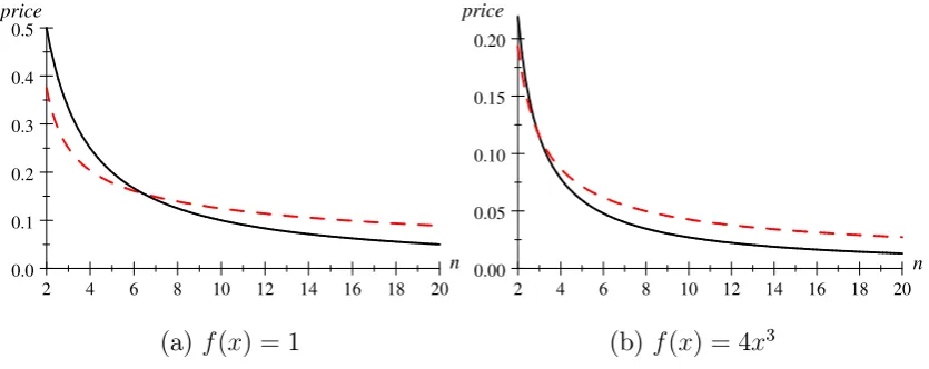
To illustrate the cut-o¤ result, consider two examples which satisfy all the conditions needed in result (ii). In the uniform distribution example with f(x) = 1, P=m < p if
n 6. Figure 2(a) below describes how both prices vary with n (where the solid curve
24Notice that we are calculatingP=minstead of the bundle priceP. So a …rm’s marginal consumers
in the bundling case are those who will switch when the …rm changesP=m by a small".
25Nalebu¤ (2000) shows a similar result in a multi-dimensional Hotelling model with two …rms, an
arbitrary number of products, and consumers uniformly distributed inside a hypercube.
26As we discussed in footnote 21, when n is large the equilibrium price p is proportional to
ispand the dashed one isP=m). In the example with an increasing densityf(x) = 4x3,
as described in Figure 2(b) below P=m < p only if n = 2. These examples show that the thresholdn^ can be small.
2 4 6 8 10 12 14 16 18 20 0.0
0.1 0.2 0.3 0.4 0.5
price
n
(a)f(x) = 1
2 4 6 8 10 12 14 16 18 20 0.00
0.05 0.10 0.15 0.20
price
n
[image:17.595.90.508.144.310.2](b)f(x) = 4x3
Figure 2: Price comparison with m= 2
Result (ii) in Proposition 1 requiresf(x)>0. Iff(x) = 0 (wherexcan be in…nity), then f(x) =g(x) and the result may not hold any more. For instance, in the example of normal distribution where limx!1f(x) = 0, bundling always lowers market prices.
Example of normal distribution. We already know that with full market coverage, shifting the support of the match utility distribution does not a¤ect the equilib-rium price. So let us normalize the mean to zero and suppose xji s N(0; 2).
Then the separate sales price de…ned in (1) is
p=
nR11 (x)d (x)n 1 ; (7)
where and are the CDF and density function of the standard normal distribu-tionN(0;1), respectively. The de…nition ofXj implies thatXj=msN(0; 2=m).
Thus,Xj=m=xj i=
p
m <disp x
j
i, so result (i) in Lemma 2 impliesP=m < p. That
is, in this example bundling always reduces market prices (and so pro…ts) regard-less ofn andm.27 A more precise relationship between the two prices is available:
Firm j’s demand in the bundling regime, when it unilaterally deviates to price
P0, is
Q(P0) = Pr[X
j
m P0
m >maxk6=j f Xk
m P
mg] = Pr[x j i
P0
p
m >maxk6=j fx k i
P
p
mg] :
27However, for any truncated normal distribution with a …nite upper bound, result (ii) in Proposition
This equals the demand for …rmj’s product i in the separate sales regime when …rmj charges P0=pm and other …rms charge P=pm. Then we deduce that
P
p
m =p : (8)
In this normal distribution example, bundling also makes the right tail thinner (i.e.,
g(x)< f(x) for large x) and the (average) position of marginal consumers also moves to the right as n increases. However, with an unbounded support the relative moving speed now matters. The density tail is higher in the separate sales case, and so it is more likely to have a high valuation draw. This implies that the position of marginal consumers moves to the right faster in the separate sales regime than in the bundling regime. Hence, even if f(x) > g(x), it is possible that f(^xf) < g(^xg) where x^f and
^
xg denote the (average) position of marginal consumers in the separate sales and the
bundling regime, respectively. This cannot happen if the upper bound x is …nite and
f(x)> g(x). In that case, when n is large bothx^f and x^g will be close tox, and so we
must have f(^xf)> g(^xg). Nevertheless, in the case with an in…nite upper bound, even
if bothx^f and x^g move to in…nity they can still be su¢ciently far away from each other
such thatf(^xf)< g(^xg).
The key feature in the normal distribution example is that xji and Xj=m belong
to the same class of distributions, such that the dispersive order result in Lemma 2 can apply. More generally this is a property of stable distributions.28 Three notable
examples of stable distributions are normal, Cauchy, and Lévy. Suppose xji has a stable distribution with a stability parameter 2(0;2]and a location parameter zero. (Normal distribution has = 2, Cauchy distribution has = 1, and Lévy distribution has = 1=2.) Then using the results in Chapter 1.6 in Nolan (2015) one can show that
Xj=m = m1 1xj
i. Therefore, Xj=m disp x
j
i and bundling reduces market prices if
1. (In the edge case with = 1, i.e., with the Cauchy distribution, bundling does not a¤ect market prices.) If <1, bundling raises market prices. (Note that this does not contradict with the duopoly result in Proposition 1 because a stable distribution with <1does no longer have a log-concave density.)29
Finally, we want to point out that f(x) > 0 (or a …nite x) is not necessary for bundling to raise market prices even if we keep the log-concavity condition. For instance, consider the distribution with a log-concave density f(x) = 2(1 x) on [0;1]. In this example,f(x) = 0, but numerical simulations suggest a similar price comparison result
28Letx
1andx2be independent copies of a random variablex. Thenxis said to bestable if for any
constantsa >0 andb >0the random variableax1+bx2has the same distribution ascx+dfor some
constantsc >0 andd.
29All the discussion here is subject to the quali…cation that for some stable distributions, the
as in Figure 2 (though the threshold ^n is bigger).30 There are also examples with x=1and a log-concave density where bundling can raise market prices. For instance, consider the generalized normal distribution with densityf(x) = 2 (1= )e jxj , where
is the shape parameter and the support is the whole real line. (The density function is log-concave when >1.) This distribution becomes the standard normal when = 2, and it converges to the uniform distribution on[ 1;1]when ! 1. Supposen^ is the threshold in the case of uniform distribution with support[ 1;1]. Then for anyn >n^, there must exist a su¢ciently large such that bundling raises market prices.
4.3
Comparing consumer surplus and total welfare
With full market coverage, consumer payment is a pure transfer and so total welfare (which is the sum of …rm pro…ts and consumer surplus) only re‡ects the match quality between consumers and products. Since pure bundling eliminates the opportunities for consumers to mix and match, it must reduce match quality and so total welfare.
However, the comparison of consumer surplus can be more complicated. If pure bundling increases market prices, then it must harm consumers since consumers su¤er from both higher prices and having no opportunities to mix and match. The trickier situation is when pure bundling lowers market prices (e.g., when n = 2, m is large, or the distribution is normal). In that case there is a trade-o¤ between the negative match quality e¤ect and the positive price e¤ect. The main message in this section is that even if bundling intensi…es price competition, the negative match quality e¤ect often dominates such that bundling harms consumers when the number of …rms is above a usually small threshold.
The per-product consumer surplus in the regime of separate sales and pure bundling are respectively
E max
j fx j
ig p and E maxj
Xj m
P m :
Then pure bundling bene…ts consumers if and only if
E max
j fx j
ig E max
j
Xj
m < p P
m : (9)
The left-hand side (which must be positive) re‡ects the match quality e¤ect, and the right-hand side is the price e¤ect.
Proposition 2 Supposef is log-concave.
(i) For a …xed m, if f(x) > 0, or if limx!xdxd(1fF(x()x)) = 0, there exists n^ such that
bundling harms consumers if n >n^. 30In fact, it can be shown that iff(x) = 0butf0
(ii) There exists n such that (a) for n n , there exists m^(n) such that bundling bene…ts consumers if m > m^(n), and (b) for n > n , there exists m^(n) such that bundling harms consumers if m >m^(n).
From the price comparison result (ii) in Proposition 1, we know that if f(x) > 0
bundling will raise prices (and so harm consumers) when n is su¢ciently large. If
f(x) = 0 (e.g., when x = 1), bundling may lower prices. But the negative match quality e¤ect will always dominate whenn is su¢ciently large if the second condition in result (i) holds (which is true for many often used distributions such as normal, exponential, extreme value, and logistic). The is easy to understand when x =1. In that case, the di¤erence between E maxjfxjig and E
h maxj
n
Xj
m
oi
can go to in…nity as n! 1, while the price di¤erence is always …nite since both prices decrease with n
under the log-concavity condition.
Result (ii) says that in the limit case withm ! 1we have a stronger cut-o¤ result: pure bundling improves consumer welfare if and only if the number of …rms is below some threshold. Notice that in the limit case withm! 1we havelimm!1Xj=m=
and limm!1P=m= 0. Then for …xed n, bundling bene…ts consumers if and only if
E max
j fx j
ig < p : (10)
The match quality e¤ect on the left-hand side increases with n, while the price e¤ect decreases with n. In the proof we show that (10) holds for n = 2 but fails for a su¢ciently large n. This proves the cut-o¤ result. Intuitively, when the number of …rms increases, bundling deprives consumers of more and more opportunities to mix and match, such that eventually the match quality e¤ect dominates. The threshold
n is typically small. For example, in the uniform distribution case with F(x) = x, condition (10) simpli…es to n2 3n 2<0, which holds only for n 3.
For a smallmit appears di¢cult to prove a cut-o¤ result.31 Figure 3 below describes
how consumer surplus varies withnin the uniform distribution case whenm = 2(where the solid curve is for separate sales, and the dashed one is for bundling). The threshold is also 3.32
31For a …nitem, we have examples where bundling harms consumers even in the duopoly case. One
such example is whenm= 2 and the distribution is exponential.
32In this example, the harm of bundling will disappear eventually as n
! 1. This is because
limn!1p= limn!1P=m = 0 and limn!1E[ maxjfx j
ig] = limn!1E[maxj Xj=m ] = x. But for
a not too largen, the harm of bundling on consumers can be signi…cant. For example, when n= 10
2 4 6 8 10 12 14 16 18 20 0.2
0.4 0.6 0.8 1.0
[image:21.595.187.408.81.236.2]n CS
Figure 3: Consumer surplus comparison with uniform distribution and m= 2
A similar cut-o¤ result holds in the normal distribution example for anym 2.
Example of normal distribution. Suppose xji s N(0; 2). From (8) and (9), we
can see that pure bundling improves consumer surplus in this example if and only if
E max
j fx j
ig E max
j
Xj
m < p[1
1
p
m] : (11)
In the Appendix, we show that
E max
j fx j
ig =
2
p ; E maxj
Xj
m =
1
p
m
2
p : (12)
Then (11) simpli…es to p > . Using (7), one can check that this holds only for
n= 2;3, so the threshold is also 3.
4.4
Incentive to bundle
This section studies …rms’ incentive to bundle. Consider an extended game where …rms can choose both whether to bundle their products and what prices to set. When there are more than two products, for tractability we assume that each …rm either bundles all its products or not at all and there are no …ner bundling strategies (by which a …rm sells some products in a package but sells others separately). The pricing game where …rms adopt asymmetric partial bundling strategies is hard to analyze.
Proposition 3 Supposef is log-concave and …rms make bundling and pricing decisions simultaneously.
(i) It is a Nash equilibrium that all …rms choose to bundle their products and charge the bundle price P de…ned in (5). Whenn = 2, this is the unique (pure-strategy) Nash equilibrium if p6=P=m.
(ii) There exists n~ such that (a) for n n~, there exists m~(n) such that separate sales is not a Nash equilibrium if m >m~(n), and (b) for n > ~n, there exists m~(n) such that separate sales is also a Nash equilibrium if m >m~(n).
It is easy to understand that it is a Nash equilibrium that all …rms bundle. This is simply because in our model if a …rm unilaterally unbundles, the market situation does not change for consumers.33 In the duopoly case, it can be further shown that neither
separate sales nor asymmetric equilibria (where one …rm bundles and the other does not) can arise in the market.
When there are more than two …rms, one may wonder whether separate sales can be another equilibrium as well. Result (ii) says that when m ! 1, this is the case if and only if n is above some threshold. The intuition of why the number of …rms matters is that the more …rms in the market, the worse a …rm’s bundle appears when it unilaterally bundles. (This is not true in the duopoly case where one …rm bundling is the same as both …rms bundling.) More formally, suppose that all other …rms o¤er separate sales at price p, but …rm j bundles unilaterally. Denote by
yi max
k6=j fx k
ig (13)
the maximum match utility of product i among …rm j’s competitors. Then …rm j is as if competing withone …rm that o¤ers a bundle with match utilityY Pmi=1yi and
price mp. If …rmj charges the same bundle price mp, its demand will be
Pr(Xj > Y) Pr(Xj >max
k6=j fX k
g) = 1
n : (14)
The inequality is because Y is greater than maxk6=jfXkgstochastically, and it is strict
when n 3. Thus, without further price adjustment it cannot be pro…table for …rmj
to unilaterally bundle.
Suppose now …rm j also adjusts its price. It is more convenient to rephrase the problem into a monopoly one where a consumer’s net valuation for product i is ui xi (yi p). (Hereyi p is regarded as the outside option to producti.) If …rmj does
not bundle, then its optimal separate sales price is p and its pro…t from each product isp=n. But its optimal pro…t when it bundles is hard to calculate in general, except in the limit case with m ! 1. In this limit case, according to the law of large numbers
33This argument depends on the assumptions that consumers buy all products and for each product
…rmj can extract all surplus by charging a bundle pricem E[ui]and its per product
pro…t will be E[ui] = E[yi] +p.34 This is no greater than the separate sales pro…t
(and so …rmj has no unilateral incentive to bundle) if and only if
(1 1
n)p <E[yi] =
Z
F(x) F(x)n 1 dx : (15)
This is clearly not true for n= 2 (which is consistent with result (i) in Proposition 3). In the proof, we show that this is true if and only if n is above a certain threshold. (This argument assumesE[ui]>0. If E[ui] 0(which occurs if n is su¢ciently large),
then …rm j of course has no incentive to bundle.)
The threshold n~ in result (ii) is usually small. For instance, with a uniform distri-bution (15) becomes n2 4n+ 2 >0 and so n~ = 3. This is the same as the threshold
n in the consumer surplus comparison result in Proposition 2. This means that in this uniform example with a large number of products, separate sales is another equilibrium outcome if and only if consumers prefer separate sales to pure bundling. In other words, with a proper equilibrium selection the market itself can work well for consumers. The same is true in the normal distribution example. (But this is not generally true. We have examples, for instance, f(x) = 2(1 x), wheren~ 6=n .)
Possibility of asymmetric equilibria. With more than two …rms one may also wonder the possibility of asymmetric equilibria where some …rms bundle and the others do not. An analytical investigation into this problem is hard because the pricing equilibrium when …rms adopt asymmetric bundling strategies does not have a simple characteriza-tion.35 However, numerical analysis can be done. Let us illustrate by a uniform example
with n = 3 and m = 2. In this example, we can claim that there are no asymmetric equilibria.
The …rst possible asymmetric equilibrium is that one …rm bundles and the other two do not. In this hypothetical equilibrium, the bundling …rm chargesP 0:513 and earns a pro…t about 0:176, and the other two …rms charge a separate price p 0:317
34This simplicity of optimal pricing with many products has been explored by Armstrong (1999)
and Bakos and Brynjolfsson (1999). Fang and Norman (2006) have studied the pro…tability of pure bundling in the monopoly case with a …nite number of products. They assume that the density ofui
is log-concave and symmetric. In our model, the log-concavity is guaranteed iff is log-concave, but the density ofui is not symmetric whenn 3 (becauseyi is stochastically greater thanxi). Without
symmetry the Proschan (1965) result thatPmi=1ui=mis more peaked thanuidoes not hold any more.
(The Proschan result has been extended in various ways, but not when the density is asymmetric.) The analysis in Fang and Norman (2006), however, crucially relies on that result. That is why their monopoly result cannot be applied to our competition model directly.
35The reason is that when some …rms bundle, other …rms will treat their products as complements,
and each earns a pro…t about 0:208. But if the bundling …rm unbundles and charges the same separate price as the other two …rms, it will have a demand 13, and its pro…t will rise to about 0:211.
The second possible asymmetric equilibrium is that two …rms bundle and the third one does not. Then the situation is like all …rms are bundling. Each bundling …rm charges a bundle price P = 0:5, the third …rm charges two single-product prices such thatp1+p2 = 0:5, and each …rm has market share13. But if one bundling …rm unbundles
and o¤ers the same separate prices as the third …rm, as we already know from (14), the remaining bundling …rm will have a demand less than 13. This implies that the deviation …rm will have a demand greater than 13 and so earn a higher pro…t. (This argument actually does not depend on the uniform distribution andm= 2.)
4.5
Discussions
4.5.1 Asymmetric products and correlated valuations
We now consider a more general setting where a …rm’s m products are potentially asymmetric and their match utilities are potentially correlated. Letxj = (xj
1; ; xjm)
be a consumer’s valuations for them products at …rm j. Suppose that xj is still i.i.d. across …rms and consumers, and it is distributed according to a joint CDFF(x1; ; xm)
with support S Rm and a bounded joint density function f(x
1; ; xm). Let Fi and fi,i= 1; ; m, be the marginal CDF and density function of xji, and let[xi; xi]be its
support. Let Gand g be the CDF and density function ofXj=m, whereXj =Pm i=1x
j i
as before, and let[x; x] be its support. Allfi and g are log-concave if the joint density
functionf is log-concave. Then the equilibrium price in each regime is de…ned similarly as before:
1
pi
=n
Z xi
xi
fi(x)dFi(x)n 1; i= 1; ; m;
1
P=m =
Z x
x
g(x)dG(x)n 1 :
The limit result that limm!1P=m = 0 still holds as long as Xj=m converges to a
deterministic value as m! 1. So for a …xedn, bundling lowers market price whenm
is su¢ciently large. Under similar conditions as before, we also have the result that for a …xedm bundling raises market prices whenn is su¢ciently large. (We have not been able to extend the duopoly result in this general setting. See the online appendix for a discussion.)
Proposition 4 Supposef is log-concave. SupposeS Rm is compact, strictly convex, and has full dimension. Then for a …xed m,
(i) if fi(xi)>0, there exists n^i such that P=m > pi for n >n^i;
Proof. Our conditions imply that g(x) = 0 (e.g., see the proof of Proposition 1 in Armstrong, 1996).36 Then the results immediately follow from result (ii) in Lemma 2.
The normal distribution example can also be extended to this general case. Suppose xj N(0; ), where 2
i in is the variance of x j
i and ik in is the covariance of
(xji; xjk). Then Xj=m N(0;(Pm i=1 2i +
P
i6=k ik)=m2). According to formula (7), P < Pmi=1pi if and only if Pmi=1 2i +
P
i6=k ik < (Pim=1 i)2. Given ik i k for
any i 6= k, this condition must hold provided that at least one pair of (xji; xjk) is not perfectly correlated.
4.5.2 Without full market coverage
We now return to the baseline model but relax the assumption of full market coverage. A subtle issue here is whether the m products are independent products or perfect complements (e.g., the essential components of a system). This will a¤ect the analysis of the separate sales benchmark. If them products are independent, consumers decide whether to buy each product separately. If the m products are perfect complements, then whether to buy a product also depends on how well-matched the other products are. (With full market coverage, this distinction does not matter.) In the following we consider the case of independent products for simplicity.
Suppose now a consumer buys a product or bundle only if it is the best o¤er in the market and provides a positive surplus. To make the case interesting, let us suppose
x 0 but the mean of xji is positive, such that some consumers do not buy but the market is still active.
In the regime of separate sales, if …rm j unilaterally deviates and charges p0 for its
product i, the demand for its producti is
q(p0) = Pr[xji p0 >max
k6=jf0; x k
i pg] =
Z x
p0
F(xji p0+p)n 1dF(xji) :
One can check that the …rst-order condition for pto be the equilibrium price is
p= q(p)
jq0(p)j =
[1 F(p)n]=n F(p)n 1f(p)
| {z }
exclusion e¤ect
+Rpxf(x)dF(x)n 1
| {z }
competition e¤ect
: (16)
(Iff is log-concave, this is also su¢cient for de…ning the equilibrium price.) In equilib-rium, a consumer will leave the market without purchasing product i with probability
36Formally,g(x) = lim
"!01 G("x "), and our conditions aboutS ensure that1 G(x ") =o(").
Among the conditions, strict convexity of S excludes the possibility that the plane of Xj=m = x
F(p)n (i.e., when each product i has a valuation less than p). Given the symmetry of
…rms, the numerator in (16) is the equilibrium demand for each …rm’s producti. The denominator is the negative of the demand slope, and it now has two parts: (i) The …rst term is the standard market exclusion e¤ect. When the valuations of all other …rms’ product i are below p (which occurs with probability F(p)n 1), …rmj acts as a
monopoly. Raising its price p by" will exclude "f(p) consumers from the market. (ii) The second term is the same competition e¤ect as in the case with full market coverage (up to the adjustment that a marginal consumer’s valuation must be greater than p).
Similarly, in the bundling case the equilibrium per-product bundle price P=m is determined by the …rst-order condition:
P
m =
[1 G(P=m)n]=n G(P=m)n 1g(P=m) +Rx
P=mg(x)dG(x)n 1
; (17)
where Gand g are the CDF and density function of Xj=m as before.
Unlike the case with full market coverage, the equilibrium price in each regime is now implicitly determined in the corresponding …rst-order condition. The following result reports the condition for each …rst-order condition to have a unique solution. (See the online appendix for the proof.)
Lemma 4 Suppose f is log-concave. There is a unique equilibrium price p 2 (0; pM)
de…ned in (16), where pM is the monopoly price solvingpM = [1 F(pM)]=f(pM), and p decreases with n. Similar results hold for P=m de…ned in (17).
For a …xed n < 1, we still have limm!1P=m = 0 since Xj=m converges to the
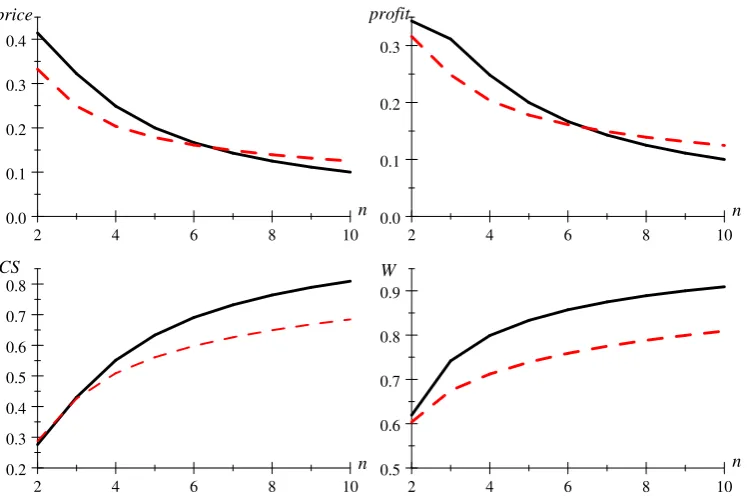
mean as m! 1. For a …xedm <1, if n is large, the demand size di¤erence between the two numerators in (16) and (17) becomes negligible and so is the exclusion e¤ect di¤erence in the denominators. Therefore, price comparison is again determined by the comparison off(x) and g(x). Intuitively, when there are many varieties in the market, almost every consumer can …nd something she likes and so almost no consumers will leave the market without purchasing anything. Then the situation will be close to the case with full market coverage. Consequently we have a similar result that when
f(x) > 0, bundling raises market prices when n is greater than a certain threshold. (We have not been able to extend the duopoly result in this setting without full market coverage.)
2 4 6 8 10 0.0
0.1 0.2 0.3 0.4
n price
2 4 6 8 10
0.0 0.1 0.2 0.3
n profit
2 4 6 8 10
0.2 0.3 0.4 0.5 0.6 0.7 0.8
n CS
2 4 6 8 10
0.5 0.6 0.7 0.8 0.9
[image:27.595.113.487.68.316.2]n W
Figure 4: The impact of pure bundling—uniform distribution example without full market coverage
An alternative way to introduce the exclusion e¤ect of price is to consider elastic demand. In the online appendix, we extend the baseline model by considering elastic consumer demand and show that the basic insights remain unchanged.
4.6
Related literature
Pure bundling or product incompatibility with product di¤erentiation. Matutes and Regibeau (1988) initiated the study of competitive pure bundling in the context of product compatibility. They study the2 2case in a two-dimensional Hotelling model where consumers are uniformly distributed on a square. They show that bundling lowers market prices and pro…ts, and it also bene…ts consumers if the market is fully covered. Our analysis in the duopoly case has generalized their results by considering more products and more general distributions.
its strongest competitor expands. This has a similar e¤ect as increasing …rm asymmetry in Hurkens, Jeon, and Menicucci (2013) and shifts the position of marginal consumers to the tail. These two papers are complementary in the sense that they point out that either …rm asymmetry or having more (symmetric) …rms can reverse the usual result that pure bundling intensi…es price competition. However, to accommodate more …rms and more products we have adopted a di¤erent modelling approach. Our model is also more general in other aspects. For example, we can allow for asymmetric products with correlated valuations, and we can also allow for a not fully-covered market or elastic demand.
In the context of product compatibility in systems markets, Economides (1989) studies a spatial model of competitive pure bundling with an arbitrary number of …rms and each selling two products. Speci…cally, consumers are distributed uniformly on the surface of a sphere and …rms are symmetrically located on a great circle (in the spirit of the Salop circular city model). He shows that for a regular transportation cost function, pure bundling always reduces market prices relative to separate sales. His spatial model features local competition: each …rm is directly competing with its two neighbor rivals only (regardless of the separate sales regime or the bundling regime),37 and they are
always symmetric to each other no matter how many …rms in total are present in the market. Conversely our random utility model features global competition: each …rm is directly competing with all other …rms. When there are more …rms, each …rm is e¤ectively competing with a stronger competitor. It is this expanding asymmetry, which does not exist in Economides’s spatial model, that drives our result that the impact of pure bundling can be reversed when the number of …rms is above a threshold.
In a recent independent work, Kim and Choi (2015) propose an alternative n 2
spatial model. They assume that consumers are uniformly distributed and …rms are symmetrically located on the surface of a torus. (Notice that …rms can be symmetrically located in many possible ways in this model.) For a quardratic transportation cost function, they show that when there are four or more …rms in the market, there exists at least one symmetric location of …rms under which making the products incompatible across …rms raises prices and pro…ts. This is consistent with our comparison result whenf(x)>0. Compared to Economides (1989), a key di¤erence in their model, using the insight learned from our paper, is that each …rm can directly compete with more …rms when the number of …rms increases if we carefully select the location of …rms. In this sense, their model is closer to our random utility model.
We have proposed a random utility approach to study competitive bundling. Our analysis has generated useful insights which can help us understand the discrepancy among the existing models and results. Whether a spatial model or a random utility model is more appropriate may depend on the context. But the random utility model