ACCEPTED FOR PUBLICATION IN Biometrics (05/07/2018)
Instrumental variable estimation in semi-parametric additive
hazards models
Matthias Brueckner
∗, Andrew Titman, and Thomas Jaki
Department of Mathematics and Statistics, Lancaster University, Lancaster LA1 4YF, U.K.
April 18, 2018
Abstract
Instrumental variable methods allow unbiased estimation in the presence of unmeasured con-founders when an appropriate instrumental variable is available. Two-stage least-squares and residual inclusion methods have recently been adapted to additive hazard models for censored sur-vival data. The semi-parametric additive hazard model which can include time-independent and time-dependent covariate effects is particularly suited for the two-stage residual inclusion method, since it allows direct estimation of time-independent covariate effects without restricting the ef-fect of the residual on the hazard. In this article we prove asymptotic normality of two-stage residual inclusion estimators of regression coefficients in a semi-parametric additive hazard model with time-independent and time-dependent covariate effects. We consider the cases of continuous and binary exposure. Estimation of the conditional survival function given observed covariates is discussed and a resampling scheme is proposed to obtain simultaneous confidence bands. The new methods are compared to existing ones in a simulation study and are applied to a real data set. The proposed methods perform favourably especially in cases with exposure-dependent censoring.
1
Introduction
Instrumental variables (IV) can be used in regression modelling to avoid bias from unmeasured con-founding or dependent measurement error in covariates by providing a source of exogenous variation (Angrist et al., 1996). These methods are also popular in epidemiology in the analysis of observational studies. In randomized clinical trials with survival endpoints unmeasured confounding may occur as a result of non-compliance, e.g. when patients switch to salvage treatment after a progression of the disease. Applying naive analysis methods in such circumstances may result in severe bias (Zeng et al., 2012).
Two-stage IV methods for duration data in econometrics have been proposed by Bijwaard and Ridder (2005). Estimation of survival probabilities under treatment non-compliance using IV methods was considered by Nie et al. (2011). Baker (1998) estimates life years saved using IV methods in the context of all-or-none compliance. Two-stage IV methods for parametric Bayesian models have been developed by Li and Lu (2015), and non-parametric binary IV methods for competing risks data by Richardson et al. (2016). The additive hazard model (Aalen, 1989) is particularly amenable to IV methods, since it resembles the linear regression model, while the popular Cox proportional hazards model is inappropriate for IV methods as shown by Tchetgen Tchetgen et al. (2015).
For additive hazard survival models with censored data several two-stage methods employing IVs have been developed. In the two-stage least squares (2SLS) method the first stage consists of a linear model for the confounded exposure given the IV and other observed covariates. In the second stage an additive hazard model is fitted with the observed exposure being replaced by the predicted exposure
from the first stage regression. Alternatively, the two-stage residual inclusion (2SRI) method (Terza et al., 2008) keeps the observed exposure in the model, but includes the estimated first stage residual as additional covariate in the model.
For the 2SRI method the first stage does not need to be a linear model, but additional assumptions about the unobserved confounding are required (Tchetgen Tchetgen et al., 2015). Essentially, in the case of continuous exposure, it is required that the unobserved confounding is a linear function of the first stage residual plus an independent error term. In the case of binary exposure we must be able to write the unobserved confounder as the sum of the conditional expectation of the unobserved confounder given exposure, instrument and observed covariates and an independent error term. These assumptions will be detailed in Section 2.
A 2SLS method for a continuous instrument for the semi-parametric additive hazard model of Lin and Ying (1994), where all covariate effects are assumed to be time-independent, was developed by Li et al. (2015). A similar 2SLS method for continuous instruments was proposed by Tchetgen Tchetgen et al. (2015) for the non-parametric additive hazard model of Aalen (1989), where all covariate effects are allowed to be time-dependent. For the same model they also develop a 2SRI method for binary and continuous instruments. However, asymptotic results are only provided for the 2SLS method. Work on IV methods for the additive hazard model has focused on the case of only time-independent covariate effects. The semi-parametric additive hazards model of McKeague and Sasieni (1994), which allows time-independent and time-dependent effects has received less attention. We argue that this model is more appropriate for the 2SRI method, since it does not require the effect of the residual included in the second stage model to be time-independent. At the same time the exposure effect can still be modelled as time-independent, which may be more useful to summarise treatment effects in a randomized trial.
While the 2SRI method requires more stringent assumptions about the influence of the unobserved confounder on the hazard, the assumptions about the censoring can be relaxed. It is sufficient that the censoring is independent of the survival time conditional on the exposure and observed covariates, since the exposure is still part of the model (Chan, 2016). While the 2SLS method with a linear first stage can be used in the case of a binary exposure, a non-linear first stage model, such as a logistic regression model, might be more appropriate.
A different and very general approach is taken by Martinussen et al. (2017), who develop an IV method for a class of structural cumulative survival models. Their approach does not require any modelling of the relationship between the exposure and the instrument. However, it requires a parametric model for conditional expectation of the instrument given the observed confounders and the survival function cannot be readily estimated from this model. In recent work Choi et al. (2017) proposed a two-stage procedure for general structural equation models, that can also be applied to censored survival data.
2
Two-stage instrumental variable methods
LetT be a continuous survival time, C the censoring time andY = min{T, C} the observed right-censored survival time. We assume that the follow-up period is a fixed finite interval [0, τ] and that the hazard ofT follows an additive hazard model
h(t|R, L, U) =α0(t) +βRR+β0LLZ+αL(t)LX+αU(U, t) (0≤t≤τ), (1) where α0 is the baseline hazard, R is the observed exposure / treatment indicator with a
time-independent effect, LZ is a p-vector of observed covariates with time-independent effects, LX is a
q-vector of observed covariates with time-dependent effects, and αU(U, t) is a term depending on a vector of unobserved confoundersU. All covariates in the model are baseline covariates which cannot change over time. We call this model the “McKeague-Sasieni model” (McKeague and Sasieni, 1994). The additive hazard model of Lin and Ying (1994) where all covariate effects are time-independent will be called the “Lin-Ying model”. The original additive hazard model of Aalen (1989) where all covariate effects are unrestricted will be called the “Aalen model”. Both the Lin-Ying and the Aalen model can be viewed as special cases of the McKeague-Sasieni model.
Our main focus is on estimating the causal effect of the exposure on the hazardβR. In general IV methods can only identify the local average treatment effect (LATE) as shown in Angrist et al. (1996), i.e. the average treatment effect of those whose exposure changes when the value of the IV changes. IV methods cannot say anything about subjects whose exposure is always the same regardless of the value of the IV (so-called “always-takers” and “never-takers” in the context of binary treatment assignement and instrument). However, implicit in Model 1 is the assumption that the treatment effectβR is the same for all individuals for a given value of the covariates. This means that the LATE is equal toβR for all subjects and can therefore be interpreted as the average treatment effect (ATE) for the entire population. Hence, the IV estimate in this model is a consistent estimate of the population ATE.
Alternatively, one could start with the Aalen model and then use ˆ
βR= 1
τ Z τ
0
ˆ
BR(t)dt
as an estimate of βR, where τ is a fixed time horizon and ˆBR(t) is a consistent estimate of the cumulative effectRt
0βR(s)dsobtained by 2SLS or 2SRI in the Aalen model (Tchetgen Tchetgen et al.,
2015). Outside of the two-stage setting this approach was also taken by Martinussen et al. (2017). However, this estimate would have a larger standard error than the semi-parametric estimate andτ
may not be data dependent. Let L = (L0
Z, L0X)0. Formally we assume the existence of an instrumental variable G, such that following assumptions hold:
(A1) Gis associated withRconditional onL.
(A2) Gis independent ofT conditional onL,R andU.
Assumption (A1) implies that there is a non-zero average causal effect of the instrument G on the exposureRand Assumption (A2) is the exclusion restriction of Angrist et al. (1996). We also assume thatLandGare exogenous, i.e.
(A3) U is independent ofL andG.
R G
L
T
[image:4.612.236.377.82.165.2]U C
Figure 1: Visualisation of IV assumptions (A1)-(A4) with instrumentG, exposureR, survival timeT, observed confoundersL, unobserved confoundersU and censoring timeC
case of a binary exposure a non-linear first stage model, such as a logistic regression model, might be more appropriate.
When considering regression methods for censored survival data it is usually necessary to assume independence of censoring and survival times conditional on all covariates included in the model. The 2SLS method requires censoringC and survival timeT to be independent conditional on the observed covariatesL. The 2SLS method can suffer from bias when censoring and survival are dependent on the exposureR. The bias of the 2SLS method induced by exposure dependent censoring is explored in Scenario VI of Li et al. (2015) and in our own simulations in Section 3. Since the exposureRis still included in the second stage model, it is sufficient to require conditional independence of censoring and survival times given the observed covariates and the exposure (Chan, 2016):
(A4) C is independent ofT conditional onR andL.
The relationships encoded in Assumptions (A1)-(A4) can be represented by a directed acyclic graph (DAG) as shown in Figure 1. The arrows represent dependencies between random variables. There is an arrow fromGtoR(Assumption (A1)), but no arrow fromGtoT (Assumption (A2)) and no arrows fromU toL and G(Assumption (A3)). The censoring C is allowed to depend on the instrument G
for 2SRI, since removing the nodesRandL from the DAG separatesT andC even whenC depends onG. It is however important to note that C must be independent from the unobserved confounder
U givenR andL, i.e. no arrow fromU toC.
2.1
Binary case
In the case of a binary exposureR we use a logistic regression model in the first stage log
p
1−p
=γ0+γGG+γL0L (2)
whereγ= (γ0, γG, γL0) andp=P(R= 1|G, L). Denote the maximum likelihood estimator ofγ by ˆγ. The predicted probability for a patient with instrumentGand covariatesLfrom this model is
ˆ
p= 1
1 + exp{−γˆ0(G, L0)0}.
The 2SRI method requires an additional linearity assumption about the unobserved heterogeneity (Tchetgen Tchetgen et al., 2015):
(A5) αU(U, t) =E{αU(U, t)|R, G, L}+(t),
where(t) is an error independent ofR,GandL. This assumption holds, for example, whenU has a normal distribution where only the mean depends onR,GandL.
Under assumptions (A1)-(A5) a reparametrization of the original model can be obtained from Result 3 of Tchetgen Tchetgen et al. (2015):
where ∆≡∆(R, G, L) =R−P(R= 1|G, L),ρ0(t) =E{αU(U, t)|R= 1, G= 0, L} −E{αU(U, t)|R= 0, G = 0, L} and ρ1(t) =E{αU(U, t)|R = 1, G= 1, L} −E{αU(U, t)|R= 0, G= 0, L} −ρ0(t). Since
the true residual ∆ is unknown it is estimated by ˆ∆ =R−pˆ.
We emphasize, that the conditional independence assumption (A4) is sufficient in the binary ex-posure case as well, i.e. censoring is allowed to be dependent on the binary exex-posure.
An interesting special case is when the exposure is confounded only for the group with G = 1, which implies thatU is independent ofR givenG= 0 and L. This is the case in our data example (Section 4) with full compliance in the control group. In this caseρ0≡0 and the conditional hazard
becomes
h(t|R, G, L) = ˜α0(t) +βRR+βL0LZ+αL(t)0LX+ρ1(t)G∆. (4)
If instead U is independent of R given G = 1 and L, then ρ1 = −ρ0 and ρ1(t)G∆ is replaced by
ρ1(t)(1−G)∆ in Eq. (4). For example, such a situation occurred in the panitumumab colorectal
cancer trial (Amado et al., 2008), where patients randomized to the standard of care group had the possibility of switching to the experimental treatment on disease progression. Fitting the model which only includes the residual-instrument interaction but not the main effect of the residual may avoid numerical stability issues as in our data example (Section 4).
We are interested in estimating the vector of regression coefficientsβ = (βR, βL0)0 and the vector of cumulative covariate effects
A(t) = Z t
0
{α˜0(s), αL(s)0, ρ0(s), ρ1(s)}0ds.
LetZ =Z(t) be then×(p+ 1) matrix withi-th row given byYi(t)(Ri, L0Zi), whereYi(t) =I(Yi≥t) is the at-risk indicator at timet of thei-th subject. Then×(q+ 3) design matrix X =X(t) for the time-dependent coefficient functions including the baseline hazard function is defined likeZ withi-th row equal toYi(t)(1, L0
Xi,∆i,∆iGi). Furthermore, we obtain the matrix ˆX= ˆX(t) by replacing inX the unknown residuals ∆ with the estimated residuals ˆ∆. We can then define the estimators ofβ and
Alike those given by McKeague and Sasieni (1994), but using ˆX instead ofX,
ˆ
β= Z τ
0
Z0HZdtˆ
−1Z τ
0
Z0HdN,ˆ (5)
and
ˆ
A(t) = Z t
0
( ˆX0Xˆ)−1( ˆX0dN−Xˆ0Zβdsˆ ), (6) where ˆH=I−Xˆ( ˆX0Xˆ)−1Xˆ0,Iis the (q+3)×(q+3) identity matrix andN(t) ={N
1(t), . . . , Nn(t)}0 =
{I(Y1≤t)δ1, . . . , I(Yn≤t)δn}0 is the vector of counting processes.
The additional variation in the second stage introduced by ˆX must be taken into account when calculating standard errors for the regression coefficients. The correct standard errors are given by Theorem 1 below. Its proof and the required regularity assumptions (B1)-(B6) are given in the Ap-pendix.
Theorem 1(2SRI, binary case). 1. Under the IV assumptions (A1)-(A5) and the regularity as-sumptions (B1)-(B3) we have
√
n( ˆβ−β) =n−1/2
n X
i=1
(iβ)+op(1), (7)
where(iβ) are iid vectors defined in Eq. (16) in the Appendix. This implies that βˆ=β+op(1)
and√n( ˆβ−β)is asymptotically normal with mean zero and covariance matrixΣβ=E((iβ)⊗2),
2. Under assumptions (A1)-(A5) and (B1)-(B6) we have
√
n( ˆA−A) =n−1/2
n X
i=1
(iA)+op(1), (8)
where(iA) are iid functions defined in Eq. (18) in the Appendix. This implies thatsuptkAˆ(t)−
A(t)k=op(1)and√n( ˆA−A)converges weakly to a vector of mean-zero Gaussian processes with
covariance functionΣA(s, t) =E{
(A)
i (s)
(A)
i (t)0}.
Theorem 1 can also be applied in the less restrictive Aalen model
h(t|R, G, L) = ˜α0(t) +{αR(t), αL(t)0}(R, L0X)
0+ρ
0(t)∆ +ρ1(t)∆G, (9)
with only time-dependent covariate effects by settingZ= 0, which implies Ψ(t) = 0 for allt.
2.2
Continuous case
For a continuous exposure we assume a linear model as the first stage model, i.e.
R=γ0+γGG+γL0L+ ∆. Assumption (A5) needs to be modified to
(A5c) αU(U, t) =ρ0(t)∆ +(t),
where(t) is an error term independent of ∆ (Tchetgen Tchetgen et al., 2015). According to Result 2 of Tchetgen Tchetgen et al. (2015) we have
h(t|R, G, L) = ˜α0(t) +βRR+βL0LZ+αL(t)0LX+ρ0(t)∆. (10)
When fitting this model the true unknown residual ∆ is again replaced with the residual from the first stage regression ˆ∆ = R−γˆ(1, G, L0)0. The result for the asymptotic distribution of Theorem 1
still holds, when we replace u1i(t) and u2i(t) with ˜u1i(t) = Yi(t) and ˜u2i(t) ≡ 0, respectively, in Assumption (B2) and (B6). As in the binary case, this holds for the special case of only time-dependent effects (Eq. (9)) as well.
2.3
Estimation of the conditional survival function
In the 2SLS approach it is possible to estimate the survival function ofT givenRandLonly, as shown by Li et al. (2015), whereas in the 2SRI approach this can only be achieved by further modelling of the conditional distribution ofGgivenRand Land then taking the expectation ofS(t|R, G, L) with respect to that distribution. This is because we can only estimate the covariate effects in the model for the conditional hazardh(t|R, L, U) (Eq. (1)), but we cannot estimate the original baseline hazard
α0(t). Therefore the survival function can only be estimated from the model for the conditional hazard
h(t|R, G, L) (Eq. (3) and Eq. (10)), which explicitly depends on the first stage residual and therefore on the instrumentG. Only in the case of binary instrument and exposure and no covariates is a simple non-parametric estimator ofS(t|R) available:
ˆ
S(t|R=r) = Pn
i=1Sˆ(t|R=r, G=g)I(Gi=g, Ri =r) Pn
i=1I(Ri =r)
.
Letδ(γ) =r−(1, g, l0
Z, l0X)γand ¯p(r, g, l) =p(r, g, l){1−p(r, g, l)}, wherep(r, g, l) = 1/[1+exp{−(1, r, g, l0)γ}]. Then
S(t|r, g, l0Z, l
0
wherex(γ) ={1, l0
X, δ(γ)}in the continuous andx(γ) ={1, l0X, δ(γ), δ(γ)g}in the binary case. Uniform consistency and asymptotic normality of the obvious estimator
ˆ
S(t|r, g, lZ, lX) = exp{−x(ˆγ) ˆA(t)−t( ˆβRr+ ˆβL0lZ)}, (11) follow from a Taylor expansion around{γ, β, A(t)} and the iid decompositions given in Theorem 2.
In principle an estimator ofS(t|r, lZ, lX) could be obtained by ˆ
S(t|r, lZ, lX) = 1
n
n X
i=1
ˆ
S(t|r, Gi, lZ, lX) ˆf(Gi|r, lZ, lX),
where ˆf(Gi|r, lZ, lX) is an estimator of the conditional probability density of G given R = r and
L= (l0
Z, l0X), such as a kernel density estimator, which is feasible when the dimension of the covariate vectorL is small. However, deriving the asymptotic properties of ˆS(t|r, lZ, lX) is beyond the scope of this paper.
Theorem 2. LetWn(t) =√n{Sˆ(t|r, g, lZ, lX)−S(t|r, g, lZ, lX)}. Under assumptions (A1)-(A5) and (B1)-(B6) we have
Wn(t) =n−1/2 n X
i=1
i(t, r, g, lZ, lX) +op(1), where
i(t, r, g, lZ, lX) =−S(t|r, g, lZ, lX){t(r, l0Z)
(β)
i +x(γ)
(A)
i (t)−(1, g, l0)Aq+2(t) (γ)
i } in the continuous case and
i(t, r, g, lZ, lX) =−S(t|r, g, lZ, lX)[t(r, l0Z)
(β)
i +x(γ)
(A)
i (t)
−p¯(r, g, l)(1, g, l0){Aq+2(t) +gAq+3(t)} (γ)
i ]
in the binary case, respectively, are iid random variables. The iid decomposition implies weak
con-vergence ofWn to a Gaussian process whose variance function can be consistently estimated by t7→
n−1P
iˆi(t, r, lZ, lX)
⊗2, whereˆi(t, r, g, l
Z, lX) is obtained by replacing all unknown quantities in the
definition ofi(t, r, g, lZ, lX)with their consistent estimators.
Theorem 2 follows from a Taylor expansion of ˆS(t|r, g, lZ, lX) around (γ, β, A(t)) and the iid de-compositions of√n(ˆγ−γ),√n( ˆβ−β) and√n( ˆA−A) in Theorem 1.
Simultaneous confidence bands for S(t|r, g, lZ, lX) can be obtained by ˆS(t|r, g, lZ, lX)±n−1/2qα, whereqαis such thatP(supt|Wn(t)| ≤qα) = 1−α. The distribution ofWn(t) can be approximated using a resampling approach based on the iid decomposition in Theorem 2. For independent standard normal random variablesQm
1, . . . , Qmn, given the observed data, the process ˆ
Wm(t|r, g, lZ, lX) =n−1/2 n X
i=1
ˆ
i(t, r, g, lZ, lX)Qmi ,
has the same asymptotic distribution as Wn(t) (Martinussen and Scheike, 2007, Theorem 5.4.1). Therefore the limiting distribution of Wn(t) can be approximated by the empirical distribution of
ˆ
W1, . . . ,WˆM for a large number M. The quantile qα is then obtained as the empirical quantile of supt|Wˆ1(t)|, . . . ,supt|WˆM(t)|.
3
Simulations
3.1
Scenarios
1) This scenario corresponds to Case I of Li et al. (2015). The instrumentG, unobserved confounder
U and observed confounder L are all standard normal. The exposure R is continuous and is generated from the linear modelR= 1 + 0.5G+L+U+N(0,0.22), whereL ∼N(0,1). The conditional hazard of the survival time ish(t|R, L, U) = 9.5 + 0.5R+ 0.5L+ 1.5U. The censoring time is exponential with rate 2.5.
2) Same as Scenario 1, but with exposure-dependent censoring, i.e. censoring time is now exponen-tial with rate 2.5 + 0.5R2
3) Same as Scenario 1, but linearity condition (A5c) for the confounder violated, i.e. in the first stageR= 1 + 0.5G+L+ ∆, where ∆∼N(0,0.22) andU = ∆2+N(0,1 + ∆2).
4) Slight modification of Scenario 3 from Martinussen et al. (2017) with continuous instrument
G ∼ N(2,1.52) and unobserved confounder U = 1.5Z2, where Z ∼ N(1,0.252). The binary
exposure is generated from the logistic regression model
logit{P(R= 1|G, U)}=−1 + 0.2G+U−E(U).
The conditional hazard of the survival time is h(t|R, U) = 0.05 + 0.4R+ 0.3U and censoring is uniform on [0,5].
5) This scenario corresponds to Case VII from Li et al. (2015). The instrument is binary with
P(G= 1) = 0.5. The unobserved confounderU is standard normal. The exposure is set to 1 if 1.5G+1.5U+≥0 and to 0 otherwise, whereis normal with mean 0 and standard deviation 0.2. This corresponds to a probit model. The survival time has hazardh(t|R, U) = 11+βR(t)R+1.5U whereβR(t) = 2.5 for alltand censoring is exponential with rate 2.5.
6) Same as Scenario 5, but with exposure-dependent censoring, i.e. C given Rhas an exponential distribution with rate 1/{0.1(1−R) + 0.3R}.
Our results include as special cases the additive hazards model where all effects are modelled as time-dependent. We consider a scenario with time-dependent exposure effect on the hazard.
7) The same as Scenario 4, but nowβR(t) = 2.5I(t <0.1)−2.5I(0.1≤t <0.2).
In the scenarios with binary exposure estimates were only calculated up to times where at least 15 (approx. 3-4 times the number of covariates) subjects were still at-risk, in order to avoid numerical instability with singular matrices in the calculation of the estimates.
3.2
Results
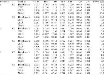
In this section we consider the results for the estimated effect of exposure. In all scenarios we also consider the coverage probability of the confidence intervals based on the unadjusted estimates of the standard errors, which do not account for the additional variation caused by including the estimated first stage residuals as covariates in the second stage. The results of the two continuous exposure Scenarios 1 and 2 are shown in Table 1. For Scenario 1 both two-stage methods can be seen to be unbiased and near nominal coverage probabilities. The naive method has a substantial bias for all sample sizes and very small coverage probability that tends to 0 as the sample size increases. In Scenario 2 with exposure-dependent censoring the 2SLS method is now biased. In Scenario 3, where the linearity assumption for the confounder is violated, 2SRI has a substantial bias, but the coverage probabilities are still close to the nominal level.
Table 1: Results of 50000 simulations for Scenarios 1-3 (continuous exposure) of benchmark (all confounders observed), two-stage residual inclusion (2SRI), two-stage least-squares (2SLS) and naive (confounders ignored) analysis for varying sample sizes n. RMSE=root mean-squared error, SD=standard deviation, ESE=estimated standard error, ESE∗=estimated unadjusted standard error of, CP=coverage probability of 95% confidence interval, CP∗=coverage probability of unadjusted 95% confidence interval
Scenario n Method RMSE Bias SD ESE ESE∗ CP CP∗ Power (%)
1 400 Benchmark 1.031 0.005 1.031 1.029 1.029 0.949 0.949 7.1
2SRI 1.124 -0.030 1.123 1.106 1.114 0.948 0.948 7.4
2SLS 1.118 -0.015 1.118 1.122 1.121 0.952 0.951 6.6
Naive 1.275 1.177 0.489 0.485 0.485 0.310 0.310 93.5 800 Benchmark 0.713 0.004 0.713 0.716 0.716 0.951 0.951 10.3
2SRI 0.775 -0.024 0.774 0.772 0.772 0.950 0.949 9.9
2SLS 0.767 -0.006 0.767 0.776 0.776 0.953 0.953 9.4
Naive 1.218 1.170 0.337 0.339 0.339 0.061 0.061 99.9
2 400 Benchmark 1.083 0.019 1.083 1.086 1.086 0.950 0.950 6.9
2SRI 1.192 0.008 1.192 1.201 1.184 0.955 0.949 6.8
2SLS 1.194 -0.137 1.186 1.184 1.182 0.949 0.949 5.2
Naive 1.287 1.173 0.530 0.530 0.530 0.390 0.390 89.2 800 Benchmark 0.753 0.006 0.753 0.757 0.757 0.951 0.951 9.8
2SRI 0.823 -0.003 0.823 0.829 0.819 0.953 0.949 9.2
2SLS 0.826 -0.136 0.815 0.818 0.818 0.949 0.949 6.6
Naive 1.225 1.168 0.369 0.370 0.370 0.109 0.109 99.5
3 400 Benchmark 1.054 0.008 1.054 1.054 1.054 0.951 0.951 6.9
2SRI 1.117 0.103 1.113 1.129 1.127 0.953 0.953 7.3
2SLS 1.127 0.010 1.127 1.128 1.128 0.951 0.951 6.5
Naive 1.047 0.007 1.047 1.048 1.048 0.951 0.951 6.9
800 Benchmark 0.734 0.001 0.734 0.733 0.733 0.951 0.951 10.3
2SRI 0.785 0.044 0.784 0.787 0.786 0.950 0.950 10.2
2SLS 0.789 -0.001 0.789 0.787 0.787 0.949 0.949 9.4
Naive 0.731 -0.001 0.731 0.731 0.731 0.951 0.951 10.2
is practically unbiased. Although, both methods have a substantially larger root mean-squared error than the benchmark method and the massively biased naive method. The results for Scenario 4 also show clearly that the unadjusted estimator underestimates standard errors resulting in coverage probabilities below the nominal level. In Scenario 5 with a probit model in the first stage the 2SRI is unbiased even though the first stage model is misspecified, while 2SLS has a small bias. In Scenario 6, which is the same as Scenario 5, but with exposure-dependent censoring 2SRI remains unbiased, while the bias of 2SLS increases. There is a notable difference in the coverage probabilities of the adjusted and unadjusted confidence intervals for the exposure effects for the 2SRI method. In the binary scenarios both IV methods do substantially increase the variance of the estimates leading to a large loss of power compared to the benchmark method. This is a general feature of the two-stage IV methods and not specific to our method.
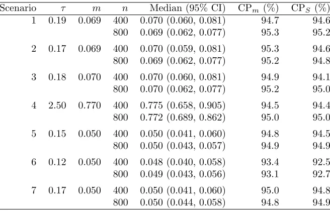
For each of the seven scenarios we also used the 2SRI method to estimate the conditional survival functionS(t|R=r, G=g, L =l) (with covariate values fixed at their mean values in the continuous scenarios). From the estimate ˆS(t|r, g, l) the median is estimated as ˆm = inf{t : ˆS(t|r, g, l) > 0.5}. The confidence interval for the median is obtained by inverting the pointwise confidence interval for
ˆ
Table 2: Results of 50000 simulations for Scenarios 4-6 (binary exposure) of benchmark (all confounders observed), two-stage residual inclusion (2SRI), two-stage least-squares (2SLS) and naive (confounders ignored) analysis for varying sample sizesn. RMSE=root mean-squared error, SD=standard deviation, ESE=estimated standard error, ESE∗=estimated unadjusted standard error of, CP=coverage proba-bility of 95% confidence interval, CP∗=coverage probability of unadjusted 95% confidence interval
Scenario n Method RMSE Bias SD ESE ESE∗ CP CP∗ Power (%)
4 400 Benchmark 0.089 -0.000 0.089 0.088 0.088 0.951 0.951 99.1 2SRI 0.236 -0.004 0.236 0.236 0.232 0.955 0.948 43.0
2SLS 0.239 0.068 0.229 0.238 0.238 0.952 0.952 51.8
Naive 0.088 -0.007 0.088 0.087 0.087 0.950 0.950 99.0 800 Benchmark 0.062 -0.001 0.062 0.062 0.062 0.950 0.950 100.0 2SRI 0.162 -0.001 0.162 0.161 0.160 0.952 0.949 70.8
2SLS 0.173 0.067 0.160 0.166 0.166 0.943 0.943 82.1
Naive 0.062 -0.007 0.061 0.061 0.061 0.949 0.949 100.0
5 400 Benchmark 2.005 0.028 2.005 1.994 1.994 0.949 0.949 24.8
2SRI 4.622 0.001 4.622 4.583 4.413 0.955 0.939 8.5
2SLS 4.766 0.117 4.765 4.775 4.767 0.955 0.954 8.2
Naive 2.668 2.211 1.493 1.480 1.480 0.674 0.674 88.8 800 Benchmark 1.395 -0.013 1.394 1.391 1.391 0.949 0.949 43.4
2SRI 3.149 0.005 3.149 3.142 3.084 0.953 0.945 13.0
2SLS 3.262 0.132 3.260 3.284 3.283 0.953 0.952 12.7
Naive 2.416 2.181 1.040 1.037 1.037 0.440 0.440 99.4 6 400 Benchmark 2.165 -0.055 2.165 2.168 2.168 0.952 0.952 21.1
2SRI 4.809 -0.031 4.809 4.769 4.192 0.950 0.899 8.1
2SLS 4.681 -0.289 4.672 4.677 4.672 0.952 0.952 7.2
Naive 2.607 2.095 1.552 1.550 1.550 0.709 0.709 82.8 800 Benchmark 1.518 -0.021 1.518 1.518 1.518 0.951 0.951 37.8 2SRI 3.272 -0.036 3.272 3.264 3.024 0.950 0.925 11.9 2SLS 3.231 -0.266 3.220 3.238 3.237 0.951 0.951 10.4 Naive 2.379 2.116 1.087 1.088 1.088 0.495 0.495 98.2
using the bootstrap method from Theorem 2, whereτ is chosen in each scenario such that on average approx. 10% of the subjects were still at risk at timeτ.
The results are shown in Table 3. In all scenarios the median estimate has a very small bias and the coverage probabilities are close to the nominal level. Only in Scenario 6, where the linearity assumption for the confounder (Assumption (A5c)) is violated, is the coverage probability of the simultaneous confidence band markedly below the nominal level.
For Scenario 7 with the time-dependent exposure effect the mean of the cumulative effectBR(t) = Rt
0βR(s)ds is shown in Figure 2. Here the naive method is substantially biased and fails to capture
Table 3: Mean of estimated median and 95% confidence intervals of the conditional survival function
S(t|R, G, L) for Scenarios 1-7 and sample sizes n = 400 and 800 in 10000 simulations. Coverage probabilities of 95% confidence intervals for the true medianm (CPm) and simultaneous confidence bands (CPS) for the survival curve on [0, τ]. Simultaneous confidence bands are estimated from 1000 bootstrap replications.
Scenario τ m n Median (95% CI) CPm(%) CPS (%)
1 0.19 0.069 400 0.070 (0.060, 0.081) 94.7 94.6 800 0.069 (0.062, 0.077) 95.3 95.2 2 0.17 0.069 400 0.070 (0.059, 0.081) 95.3 94.6 800 0.069 (0.062, 0.077) 95.2 94.8 3 0.18 0.070 400 0.070 (0.060, 0.081) 94.9 94.1 800 0.070 (0.062, 0.077) 95.2 95.0 4 2.50 0.770 400 0.775 (0.658, 0.905) 94.5 94.4 800 0.772 (0.689, 0.862) 95.0 95.0 5 0.15 0.050 400 0.050 (0.041, 0.060) 94.8 94.5 800 0.050 (0.043, 0.057) 94.9 94.9 6 0.12 0.050 400 0.048 (0.040, 0.058) 93.4 92.5 800 0.049 (0.043, 0.056) 93.1 92.7 7 0.17 0.050 400 0.050 (0.041, 0.060) 95.0 94.8 800 0.050 (0.044, 0.058) 94.8 94.9
4
Application
We consider data from a social experiment conducted by Illinois Department of Employment Security between mid-1984 and mid-1985 to test the effect of cash bonuses in reducing the duration of insured unemployment (W.E. Upjohn Institute, 1987; Woodbury and Spiegelman, 1987). A total of 12101 new claimants for unemployment insurance were randomized into 3 groups, 3952 to the control group (no cash bonus offered), 3963 to the employer bonus group (cash bonus offered to the next employer), and 4186 to the claimant bonus group (cash bonus offered to the claimant). The cash bonus of $500 was only paid if the the claimants found a new job within 11 weeks of claiming unemployment insurance. Thus, it is plausible to assume that the effect of offering the bonus on the duration of unemployment is time-dependent.
We will only analyse the data from the claimant bonus experiment consisting of the control group and the claimant bonus group. Subjects randomized to the control group were not informed about the experiment and not asked whether they wanted to participate. In the claimant bonus group 659 (15.7%) refused to participate for unknown reasons, which suggests that there is unobserved confounding.
This dataset has been previously analysed using a two-stage IV method based on a mixed pro-portional hazards model using the original randomization as the instrument (Bijwaard and Ridder, 2005). We analyse the dataset using the 2SLS and 2SRI methods, both with the cash bonus offer effect modelled as time-dependent and time-independent, and the naive method without any adjustment. The 2SRI is implemented based on the model in Eq. (4), which does not include the main effect of the first stage residual, since including the main effect made the design matrix singular for all event times. Following Bijwaard and Ridder (2005) we include age, the logarithm of pre-unemployment earnings, gender, ethnicity, and the logarithm of the weekly amount of unemployment insurance benefits plus dependence allowance as additional covariates in our first and second stage models.
0.0 0.2 0.4
0.00 0.05 0.10 0.15 0.20 0.25 Time
Cum
ulativ
e e
xposure eff
ect
[image:12.612.151.462.85.287.2]Method True 2SRI Naive Benchmark
Figure 2: Results of Scenario 7. Mean of ˆBR(t) fort∈[0,0.25] of 10000 simulations with sample size
n= 1000.
goodness-of-fit test indicates that the additive hazard model fits the data well for the female subgroup (p = 0.14), but neither the male subgroup (p= 0.006) nor the entire group (p = 1.7×10⁻⁵). We
therefore restrict our analysis to the 3619 female participants in the claimant bonus experiment. The estimated cumulative effects are shown in Web Figure 2 in Web Appendix A. The non-parametric two-stage estimates are slightly larger than the non-non-parametric naive estimate. The 2SRI method in the McKeague-Sasieni model and the 2SLS method in the Lin-Ying model give practi-cally identical results for the effect of the cash bonus offer with the estimated effect 2.84×10⁻³with
standard error 1.19×10⁻³ about 77.5% larger than the naive estimate 1.60×10⁻³ with standard error 1.02×10⁻³. All estimates are positive, i.e. offering the cash bonus increases the hazard of re-employment therefore shortening the duration of uninsurance benefit claims, as expected.
The estimated effect for the 2SRI method is statistically significant (p= 0.008), but not for the naive method (p= 0.059).
5
Discussion
We have provided asymptotic results for the two-stage residual inclusion method in an semi-parametric additive hazard model for binary and continuous exposure. These results include as a special case the general model where all effects are time-dependent. The advantage of the semi-parametric model in connection with 2SRI method is that the effect of the included residual may be time-dependent, while the effect of other covariates can modelled as constant over time.
Our simulations have shown that the 2SRI method avoids the bias of 2SLS when censoring depends on the exposure and when the first stage is a non-linear model. Although the asymptotic results assume a logistic regression model in the first stage, an extension to other generalized linear models would be straightforward. The coverage probabilities of the confidence intervals are near the nominal level even for relatively small sample sizes and the method is seen to be robust when the data is generated from a probit model in the first stage instead of the assumed logistic model. The naive method, which ignores any confounding, had in some cases a very large bias and coverage probabilities far below the nominal level.
It can be seen that the coverage probabilties of the confidence intervals based on the unadjusted standard errors can be substantially below the nominal level. This is despite the difference between the adjusted and unadjusted standard errors seemingly becoming smaller as the sample size increases.
Acknowledgements
This work is independent research arising in part from Dr Jaki’s Senior Research Fellowship (NIHR-SRF-2015-08-001) supported by the National Institute for Health Research. Funding for this work was also provided by the Medical Research Council (MR/M005755/1). The views expressed in this publication are those of the authors and not necessarily those of the NHS, the National Institute for Health Research or the Department of Health.
Supplementary Materials
Figures referenced in Sections 3 and 4 and the R code (R Core Team, 2017) for fitting the two-stage methods to the data set in Section 4 are available with this paper at the Biometrics website on Wiley Online Library.
References
Aalen, O. O. (1989). A linear regression model for the analysis of life times. Statistics in Medicine, 8(8):907–925.
Amado, R. G., Wolf, M., Peeters, M., Van Cutsem, E., Siena, S., Freeman, D. J., Juan, T., Sikorski, R., Suggs, S., Radinsky, R., Patterson, S. D., and Chang, D. D. (2008). Wild-type KRAS is required for panitumumab efficacy in patients with metastatic colorectal cancer. Journal of Clinical Oncology, 26(10):1626–1634.
Andersen, P. K., Gill, R. D., and Keiding, N. (1993). Statistical Models Based on Counting Processes. Springer Science & Business Media.
Angrist, J. D., Imbens, G. W., and Rubin, D. B. (1996). Identification of Causal Effects Using Instrumental Variables. Journal of the American Statistical Association, 91(434):444–455.
Baker, S. G. (1998). Analysis of Survival Data from a Randomized Trial with All-or-None Compli-ance: Estimating the Cost-Effectiveness of a Cancer Screening Program. Journal of the American
Statistical Association, 93(443):929–934.
Bijwaard, G. E. and Ridder, G. (2005). Correcting for selective compliance in a re-employment bonus experiment. Journal of Econometrics, 125(1):77–111.
Chan, K. C. G. (2016). Reader reaction: Instrumental variable additive hazards models with expo-suredependent censoring. Biometrics, 72(3):1003–1005.
Choi, B. Y., Fine, J. P., and Brookhart, M. A. (2017). On two-stage estimation of structural instru-mental variable models. Biometrika, 104(4):881–899.
Gandy, A. and Jensen, U. (2005). On Goodness-of-Fit Tests for Aalen’s Additive Risk Model.
Scan-dinavian Journal of Statistics, 32(3):425–445.
Lenglart, E. (1977). Relation de domination entre deux processus. InAnnales de l’IHP Probabilits et
statistiques, volume 13, pages 171–179.
Li, J., Fine, J., and Brookhart, A. (2015). Instrumental variable additive hazards models. Biometrics, 71(1):122–130.
Lin, D. Y. and Ying, Z. (1994). Semiparametric analysis of the additive risk model. Biometrika, 81(1):61–71.
Martinussen, T. and Scheike, T. H. (2007). Dynamic Regression Models for Survival Data. Springer Science & Business Media.
Martinussen, T., Vansteelandt, S., Tchetgen, T., J, E., and Zucker, D. M. (2017). Instrumental variables estimation of exposure effects on a time-to-event endpoint using structural cumulative survival models. Biometrics, 73(4):1140–1149.
McKeague, I. W. and Sasieni, P. D. (1994). A Partly Parametric Additive Risk Model. Biometrika, 81(3):501–514.
Nie, H., Cheng, J., and Small, D. S. (2011). Inference for the Effect of Treatment on Survival Probability in Randomized Trials with Noncompliance and Administrative Censoring. Biometrics, 67(4):1397– 1405.
R Core Team (2017). R: A Language and Environment for Statistical Computing. R Foundation for Statistical Computing, Vienna, Austria.
Richardson, A., Hudgens, M. G., Fine, J. P., and Brookhart, M. A. (2016). Nonparametric binary instrumental variable analysis of competing risks data. Biostatistics, page kxw023.
Tchetgen Tchetgen, E. J., Walter, S., Vansteelandt, S., Martinussen, T., and Glymour, M. (2015). Instrumental variable estimation in a survival context.Epidemiology (Cambridge, Mass.), 26(3):402– 410.
Terza, J. V., Basu, A., and Rathouz, P. J. (2008). Two-Stage Residual Inclusion Estimation: Address-ing Endogeneity in Health Econometric ModelAddress-ing. Journal of Health Economics, 27(3):531–543. W.E. Upjohn Institute (1987). The Illinois Unemployment Insurance Experiments public use data.
https://upjohn.org/node/950. Accessed: 2017-06-29.
Woodbury, S. A. and Spiegelman, R. G. (1987). Bonuses to Workers and Employers to Reduce Unem-ployment: Randomized Trials in Illinois. The American Economic Review, 77(4):513–530.
Zeng, D., Chen, Q., Chen, M.-H., Ibrahim, J. G., and Groups, A. R. (2012). Estimating treatment effects with treatment switching via semicompeting risks models: an application to a colorectal cancer study. Biometrika, 99(1):167–184.
A
A.1
First stage iid decompositions
We state two well known asymptotic results for the maxmium-likelihood estimators for the logistic and linear regression models, that we need for our proof of Theorem 1. We have
√
n(ˆγ−γ) =n−1/2
n X
i=1
(iγ)+op(1), (12)
where(iγ) (i = 1, . . . , n) are independent and identically distributed mean-zero random (p+q+ 2)-vectors.
1. Logisitic regression: (iγ)=V
−1
1 (1, Gi, L0i)0∆i, whereV1=−E{p(1−p)(1, G, L0)0(1, G, L0)}.
2. Linear regression: (iγ)=V
−1
A.2
Regularity assumptions
A number of regularity assumptions are needed for proving our asymptotic results: (B1) There exist positive definite (p+1)×(p+1) matrices Ω and Σ such thatn−1Rτ
0 Z(t)
0H(t)Z(t)dt−→p
Ω andn−1Rτ
0 Z(t)
0H(t)diag{dN(t)}H(t)0Z(t)−→p Σ, whereH =I−X(X0X)−1X0.
(B2) Fork= 1,2 exist positive definite matrices Γ1k such that
n−1
Z τ
0
Z(t)0H(t)diag{uk(t)}X1dA(q+1+k)(t)
p
−→Γ1k,
whereX1 is then×rdesign matrix of the first stage regression, andu1(t) andu2(t) are vectors
defined byu1i(t) =pi(1−p1)Yi(t) andu2i(t) =u1i(t)Gi, respectively. Let Γ1= Γ11+ Γ12.
(B3) The covariatesR, GandLhave bounded support.
In order to prove uniform consistency ofAand convergence of√n( ˆA−A) to a mean-zero Gaussian process we need the following additional assumptions:
(B4) There exists a positive definite (q+ 3)×(q+ 3) matrix function ξ(t) such that
nsup t
k
Z t
0
{X(s)0X(s)}−1X(s)0diag{dN(s)}X(s){X(s)0X(s)}−1−ξ(t)k−→p 0.
(B5) There exists positive definite (p+ 1)×(q+ 3) matrices Ψ(t) such that sup
t
k
Z t
0
{X(s)0X(s)}−1X(s)0Z(s)ds−Ψ(t)k p
−→0,
wherekAk= maxiPj|aij|for a matrixA= (aij).
(B6) Fork= 1,2 andt∈[0, τ] exist positive definite matrices Γ2k(t) such that sup
t
kn−1 Z t
0
{X(s)0X(s)}−1X(s)0diag{uk(s)}X1dA(q+1+k)(s)−Γ2k(t)k p
−→0.
Let Γ2(t) = Γ21(t) + Γ22(t) fort∈[0, τ].
Furthermore, we also assume the regularity conditions required for asymptotic normality of the maximum-likelihood estimator ˆγin the logistic regression model. Specifically, we assume that
√
n(ˆγ−γ) =n−1/2
n X
i=1
(iγ)+op(1), (13)
where(iγ) are iid random variables defined in the Appendix with covariance matrixK=E(
(γ)0
i
(γ)
i ).
A.3
Proofs
Lemma 1. Under Assumptions (B1), (B3) and (B4)
n−1/2 Z τ
0
Z0Hˆ( ˆX−X)dA=−Γ1n−1/2
n X
j=1
(jγ)+op(1),
and
n−1/2 Z t
0
( ˆX0Xˆ)−1Xˆ0( ˆX−X)dA=−Γ2(t)n−1/2
n X
j=1
Proof. We only prove the first equation, the proof of the second is almost identical. We have ˆX(t) =
X(t) +{0n×(q+1), v1(t), v2(t)}, wherev1i(t) =Yi(t)( ˆ∆i−∆i) =−Yi(t)(ˆpi−pi) and v2i(t) =v1i(t)Gi.
The delta method implies√n(ˆpi−pi) =pi(1−pi)(1, Gi, L0i)
√
n(ˆγ−γ) +op(1). Therefore
n−1/2Rτ
0 Z
0Hˆ( ˆX−X)dA =n−1/2Rτ
0 Z
0Hˆ{v1(t)dA(q+2)(t) +v2(t)dA(q+3)(t)} =−n−1Rτ
0 Z
0Hˆ
diag{u1(t)}X1dA(q+2)(t) + diag{u2(t)}X1dA(q+3)(t)
√
n(ˆγ−γ) +op(1)
Since the covariates are bounded and ˆγ=γ+op(1) we have suptkZ0Hˆ−Z0Hk=op(1). The conclusion
then follows by Assumption (B3) and Eq. (13).
Proof of Theorem 1. LetM = (M1, . . . , Mn)0 be the vector of counting process martingales, where
Mi(t) =Ni(t)− Z t
0
Yi(s)h(s)ds. We have
Rτ
0 Z
0HdMˆ =Rτ
0 Z
0HdNˆ −Rτ
0 Z
0HXdAˆ −Rτ
0 Z
0HZdtβˆ =Rτ
0 Z
0HdNˆ +Rτ
0 Z
0Hˆ( ˆX−X)dA−Rτ
0 Z
0HZdtβˆ since ˆHXˆ = 0. Thus
√
nβ=
n−1 Z τ
0
Z0HZdtˆ −1
n−1/2 Z τ
0
Z0HdNˆ + Z τ
0
Z0Hˆ( ˆX−X)dA−
Z τ
0
Z0HdMˆ
,
and with the definition of ˆβ in Eq. (5) we have
√
n( ˆβ−β) = n−1Rτ
0 Z
0HZdtˆ −1n−1/2Rτ
0 Z
0HdMˆ
−n−1Rτ
0 Z
0HZdtˆ −1n−1/2Rτ
0 Z
0Hˆ( ˆX−X)dA (14)
Since suptkXˆ(t)−X(t)k = op(1) we have suptkn−1Z0HZˆ −n−1Z0HZk = op(1). By Assump-tion (B1) and Lemma 1 the second term on the right hand side becomes
Ω−1Γ1n−1/2
n X
j=1
(jγ)+op(1), (15)
which is a sum of mean-zero iid terms and asymptotic normality follows from the central limit theorem. Asymptotic normality of the first term on the right hand side of Equation (14) follows from the martingale central limit theorem (Andersen et al., 1993). The asymptotic variance of √n( ˆβ −β) follows, since the two terms on the right hand side of Equation (14) are asymptotically independent. Thus, Σβ = Ω−1{Σ + Γ1KΓ01}Ω−1.
For later reference we note that √n( ˆβ−β) admits the following iid decomposition√n( ˆβ−β) =
n−1/2P i
(β)
i +op(1), where
(iβ)= Ω
−1Z
τ
0
{Z·0i(t)−ψ(t)0X·0i(t)}dMi(t) + Ω−
1
Γ1 (γ)
i , (16) whereψ(t)0=Z(t)0X(t){X(t)0X(t)}−1.
Now let ˆQ= ( ˆX0Xˆ)−1Xˆ0, Q= (X0X)−1X0. For showing asymptotic normality of ˆA we start by
noting that
√
n{Aˆ(t)−A(t)}= √nRt
0QdNˆ −
Rt
0QZdsˆ
√
n( ˆβ−β)
−√nRt
0QˆXdAˆ −
√
nRt
0QZβdsˆ +op(1)
= √nRt
0QdMˆ −
√
nRt
0Qˆ( ˆX−X)dA−
Rt
0QZdsˆ
√
The second term on the right hand side is asymptotically equivalent to Γ2(t)n−1/2P
n j=1
(γ)
j , by Lemma 1, and the last term is asymptotically equivalent to−Ψ(t)0n−1/2P
i
(β)
i by Assumption (B2) and Eq. (15). Thus,
√
n{Aˆ(t)−A(t)}=√n Z t
0
ˆ
QdM−Ψ(t)0n−1/2
n X
i=1
(iβ)+ Γ2(t)n−1/2
n X
j=1
(jγ)+op(1). (17)
The martingale central limit theorem and Assumption (B3) imply convergence of the first term on the right hand side to a mean-zero Gaussian process with covariation function (s, t)7→ξ(s∧t). The second term converges to a mean-zero Gaussian process Ψ(·)0mβ where mβ is a mean-zero normal random vector with covariance matrix Ω−1ΣΩ−1. The last term on the right hand side converges to a mean-zero Gaussian process {Γ2(·)−Ψ(·)0Ω−1Γ1}mr where mr is a mean-zero normal random vector with covariance matrixK. All three processes are asymptotically independent, since each(jγ)is time-independent and the covariation between the two martingale processes is 0, by a similar argument as that in Appendix 1 of McKeague and Sasieni (1994). Thus, ΣA(s, t) = ξ(s∧t) + Ψ(s)ΣβΨ(t)0+ Γ2(s)KΓ2(t)0.
In order to prove uniform consistency of ˆAon [0, τ] we divide Eq. (17) by√nand see that all terms converge to 0 uniformly in probability, the first two terms by Lenglart’s inequality (Lenglart, 1977) and the last term because of the law of large numbers.
We have again an iid decomposition√n{Aˆ(t)−A(t)}=n−1/2P i
(A)
i (t) +op(1), where
(iA)(t) = Z t
0
V−1X0
·idMi−Ψ(t)0
(β)
i + Γ2(t) (γ)


![Figure 2: Results of Scenario 7. Mean of ˆnBR(t) for t ∈ [0, 0.25] of 10000 simulations with sample size = 1000.](https://thumb-us.123doks.com/thumbv2/123dok_us/9302467.429950/12.612.151.462.85.287/figure-results-scenario-mean-nbr-simulations-sample-size.webp)
