Analogue Dynamics Engine (ADE)
Final Year Project 2005
Muiris Woulfe
B.A. (Mod.) Computer Science Supervisor: Michael Manzke
Acknowledgements
I would like to express my gratitude to my supervisor, Michael Manzke, for his helpful advice and guidance throughout the project.
Additionally, I would like to take this opportunity to sincerely thank my parents for their continued support throughout my time at college.
Abstract
This report outlines the design and implementation of the Analogue Dynamics Engine (ADE). The ADE is a physics engine constructed from a hybrid, ana-logue and digital, computer. Software physics engines are becoming increas-ingly common in computer games, and the ADE was designed as a hardware equivalent to these software engines. Analogue computers, although currently rare, have useful properties such as their ability to evaluate functions in real-time. The physics engine exploits this functionality while using digital compo-nents to provide reconfigurability.
The core hybrid computer was constructed by connecting twenty nine cus-tom designed reconfigurable analogue cells to thirty two bus lines, using pro-grammable interconnect. Each cell can perform inversion, integration, addition and multiplication. At the periphery of this computer lie two ADCs and two DACs, so that the hybrid computer may provide a digital interface.
In order to make the engine suitable for use with games, it was decided to make simulations multiplexable, so that multiple simulations could be run “concurrently”. This requires simulations to be executed faster than real-time. Additionally, state must be saved and restored, which was achieved through replicating the capacitors.
Finally, this report analyses the viability of this project for use in computer games. Ultimately, it was determined that an analogue computer could be-come a viable replacement for the software physics engines in use today. In fact, it offers benefits that cannot be obtained using today’s software physics engines.
Contents
Acknowledgements
ii
Abstract
iii
Contents
iv
List of Figures
ix
List of Tables
xii
List of Code
xiii
CD Contents
xiv
I
Background
1
1 Introduction 2
1.1 Project Overview . . . 2
1.1.1 Physics Engine . . . 2
1.1.2 Dedicated Hardware . . . 2
1.1.3 Analogue Computer . . . 3
1.1.4 Hybrid Computer . . . 3
1.1.5 Project Definition . . . 4
1.2 Advantages . . . 4
2 Physics Engines 5 2.1 Overview. . . 5
2.2 History . . . 5
2.3 Available Engines . . . 6
2.4 Applications . . . 7
2.4.1 Engineering Analyses . . . 7
2.4.2 Computer Games . . . 7
2.5 Advantages . . . 8
CONTENTS v
2.5.1 Realism . . . 8
2.5.2 Expertise. . . 8
2.5.3 Expense . . . 8
3 Analogue Computers 10 3.1 Overview. . . 10
3.2 History . . . 10
3.3 Applications . . . 12
3.3.1 Simulation . . . 12
3.3.2 Control . . . 13
3.4 Advantages . . . 13
3.4.1 Real-Time . . . 13
3.4.2 Parallelism. . . 14
3.4.3 Potentially Infinite Accuracy . . . 15
3.5 Disadvantages . . . 15
3.5.1 Noise . . . 15
3.5.2 Inflexibility . . . 16
3.5.3 Not Dynamically Reconfigurable . . . 16
4 Hybrid Computers 17 4.1 Overview. . . 17
4.2 History . . . 17
4.3 Applications . . . 18
4.4 Advantages . . . 18
4.4.1 Reconfigurability . . . 18
4.4.2 Leveraging Analogue and Digital . . . 19
4.5 Disadvantages . . . 19
4.5.1 Noise . . . 19
5 Analogue 20 5.1 Overview. . . 20
5.2 Applications . . . 20
5.2.1 Wireless Communications . . . 20
5.2.2 Wireline Communications . . . 22
5.2.3 Sensors . . . 22
5.2.4 Disk Drives . . . 22
5.2.5 Microprocessors and Memories. . . 23
5.2.6 Game Controllers . . . 23
5.2.7 Zoom . . . 23
6 Operational Amplifiers 24 6.1 Overview. . . 24
6.2 History . . . 24
6.3 Terminals. . . 25
6.4 Ideal Operational Amplifier . . . 26
6.5 Practical Operational Amplifier . . . 27
6.6 Circuits . . . 27
6.6.1 Inverter . . . 27
6.6.2 Multiplier and Divider . . . 28
CONTENTS vi
6.6.4 Integrator . . . 29
6.6.5 Differentiator . . . 30
6.6.6 Logarithm Calculator . . . 32
6.6.7 Antilogarithm Calculator . . . 33
6.6.8 Further Operations . . . 33
II
Design and Implementation
34
7 Implementation Background 35 7.1 VHDL-AMS . . . 357.2 Software . . . 36
7.2.1 Mentor Graphics’ SystemVision . . . 36
7.2.2 Xilinx ISE . . . 36
7.3 Behavioural and Structural . . . 36
7.4 Testbenches . . . 37
8 Prototype 1: Mass-Spring-Damper 38 8.1 Background . . . 38
8.1.1 Physics of Mass-Spring . . . 38
8.1.2 Physics of Mass-Spring-Damper . . . 40
8.2 Voltage Sources . . . 41
8.2.1 Voltage Source . . . 41
8.2.2 Sinusoidal Voltage Source . . . 41
8.3 Packages . . . 42
8.3.1 Arithmetic . . . 42
8.3.2 Constants . . . 43
8.3.3 Type Conversion . . . 43
8.3.4 Types . . . 43
8.4 Core Entities . . . 43
8.4.1 Resistor . . . 44
8.4.2 Capacitor . . . 44
8.4.3 Operational Amplifier . . . 45
8.5 Derived Entities . . . 45
8.5.1 Inverter . . . 45
8.5.2 Integrator . . . 48
8.5.3 Differentiator . . . 50
8.6 Mass-Spring-Damper . . . 51
8.7 Simplified Mass-Spring-Damper . . . 53
9 Prototype 2: Vehicle Suspension System 59 9.1 Background . . . 59
9.1.1 Physics of Vehicle Suspension System . . . 59
9.2 Vehicle Suspension System. . . 60
10 Reconfigurable Hybrid Computer 65 10.1 Switch . . . 65
10.2 Variable Resistor. . . 66
10.3 Switchable Resistor . . . 66
CONTENTS vii
10.5 Cell . . . 67
10.6 Hybrid Systems . . . 69
10.7 Router . . . 69
10.8 Cell Router. . . 72
10.9 Computer . . . 72
10.10DAC . . . 73
10.11ADC . . . 77
10.12Digitised Computer. . . 78
10.13ADE. . . 80
11 Multiplexing 81 11.1 Background . . . 81
11.1.1 Key Concept. . . 81
11.1.2 Multiplexing Suggestions . . . 82
11.1.2.1 Suggestion 1: Iterating Outputs . . . 82
11.1.2.2 Suggestion 2: Simulating Change . . . 83
11.1.2.3 Suggestion 3: Capacitor Replication. . . 84
11.2 Capacitor Stack . . . 84
11.3 Cell . . . 85
11.4 Cell Router. . . 86
11.5 Computer and Digitised Computer. . . 86
11.6 Operation Decoder . . . 86
11.7 Operation Decoders. . . 86
11.8 Control Unit . . . 87
11.9 ADE. . . 87
11.10Hierarchy . . . 89
12 Problems and Solutions 93 12.1 Size . . . 93
12.2 Speed . . . 93
12.3 VHDL-AMS Standard . . . 94
12.4 Looped Back Inputs. . . 94
12.5 Resistor and Capacitor Strengths . . . 95
III
Conclusions
96
13 Synthesis 97 13.1 Discrete Components . . . 9713.2 ASICs . . . 97
13.3 FPAAs . . . 98
13.3.1 Zetex Semiconductors TRAC . . . 98
13.3.1.1 Analysis. . . 99
13.3.2 Lattice Semiconductor ispPAC . . . 99
13.3.2.1 Analysis. . . 99
13.3.3 Anadigm FPAAs . . . 99
13.3.3.1 Analysis. . . 100
13.3.4 Other FPAAs . . . 101
13.3.5 Disadvantages . . . 101
CONTENTS viii
13.5 Decision . . . 101
14 PC Interfaces 102 14.1 Peripheral Buses. . . 102
14.1.1 PCI . . . 102
14.1.2 PCIe . . . 102
14.1.3 Motherboard . . . 103
14.2 Graphics Cards . . . 103
14.3 External Device . . . 103
14.4 Conclusions . . . 104
15 Analysis 105 15.1 Interface . . . 105
15.2 Die Area . . . 106
15.3 Design . . . 110
15.4 Timing . . . 110
15.4.1 ADC Conversion Rate . . . 110
15.4.2 Operational Amplifier Bandwidth . . . 110
15.4.3 Execution Speed . . . 111
16 Conclusions 113 16.1 Knowledge Acquired . . . 113
16.2 Future Work . . . 114
16.3 Summary. . . 114
List of Figures
3.1 Parallelism in analogue computers . . . 14
5.1 Analogue and digital signals . . . 21
(a) Continuous time analogue signal. . . 21
(b) Discrete time analogue signal . . . 21
(c) Digital signal . . . 21
6.1 Operational amplifier circuit symbols . . . 25
(a) Complete . . . 25
(b) Simplified . . . 25
6.2 Typical operational amplifier configuration . . . 26
6.3 Inverter . . . 28
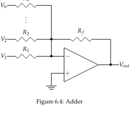
6.4 Adder. . . 28
6.5 Integrator. . . 29
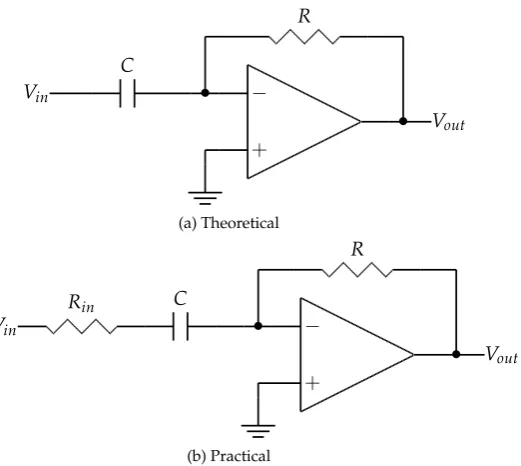
6.6 Differentiator . . . 31
(a) Theoretical. . . 31
(b) Practical . . . 31
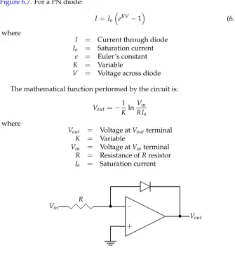
6.7 Logarithm calculator . . . 32
6.8 Antilogarithm calculator . . . 33
8.1 Mass-spring . . . 39
8.2 Behaviour of a mass-spring . . . 39
8.3 Mass-spring-damper . . . 40
8.4 Behaviour of a mass-spring-damper . . . 40
8.5 Operational amplifier in negative feedback configuration . . . . 45
8.6 Schematic of inverter . . . 46
8.7 Comparison of inverter’s behavioural and structural models . . 47
(a) Original . . . 47
(b) Magnified . . . 47
8.8 Schematic of integrator . . . 48
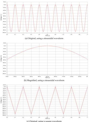
8.9 Comparison of integrator’s behavioural and structural models . 49 (a) Original, using a sinusoidal waveform . . . 49
(b) Magnified, using a sinusoidal waveform . . . 49
(c) Original, using a square waveform. . . 49
(d) Magnified, using a square waveform . . . 50
8.10 Schematic of differentiator . . . 50
8.11 Differentiator . . . 51
(a) Behavioural . . . 51
LIST OF FIGURES x
(b) Structural . . . 51
8.12 Mass-spring-damper analogue computers . . . 54
(a) Original . . . 54
(b) Optimised . . . 55
8.13 Comparison of mass-spring-damper’s behavioural and struc-tural models . . . 56
(a) Displacement in. . . 56
(b) Displacement out . . . 56
(c) Displacement out magnified . . . 56
(d) Velocity . . . 57
(e) Velocity magnified . . . 57
9.1 Walking-beam model for vehicle suspension system . . . 60
9.2 Vehicle suspension system analogue computer . . . 62
9.3 Comparison of vehicle suspension system’s behavioural and structural models . . . 63
(a) Wheel 1 input . . . 63
(b) Wheel 2 input . . . 63
(c) Displacement . . . 63
(d) Displacement magnified . . . 64
10.1 Schematic of switchable resistor. . . 66
10.2 Schematic of switchable capacitor. . . 67
10.3 Schematic of cell. . . 68
10.4 Comparison of hybrid mass-spring-damper’s behavioural and structural descriptions . . . 70
(a) Displacement out . . . 70
(b) Magnified displacement out . . . 70
(c) Velocity . . . 70
(d) Magnified velocity . . . 71
10.5 Comparison of hybrid vehicle suspension system’s behavioural and structural descriptions. . . 71
(a) Displacement . . . 71
(b) Magnified displacement . . . 71
10.6 Schematic of cell router. . . 72
10.7 Schematic of computer . . . 74
10.8 Comparison of computer’s structural mass-spring-damper test-bench against mass-spring-damper’s behavioural description . 75 (a) Displacement out . . . 75
(b) Magnified displacement out . . . 75
(c) Velocity . . . 75
(d) Magnified velocity . . . 76
10.9 Comparison of computer’s structural vehicle suspension system testbench against vehicle suspension system’s behavioural de-scription . . . 76
(a) Displacement . . . 76
(b) Magnified displacement . . . 76
10.10Schematic of digitised computer . . . 78
LIST OF FIGURES xi
(a) Displacement out . . . 80
(b) Magnified displacement out . . . 80
(c) Velocity . . . 80
(d) Magnified velocity . . . 80
10.12ADE’s structural description, using the vehicle suspension sys-tem testbench . . . 80
(a) Displacement . . . 80
(b) Magnified displacement . . . 80
11.1 Multiplexed computer using suggestion one . . . 82
11.2 Multiplexed computer using suggestion two (simplified) . . . . 83
11.3 Schematic of capacitor stack . . . 85
11.4 Schematic of multiplexed cell . . . 85
11.5 Schematic of multiplexed ADE . . . 87
11.6 ADE’s structural model, using the mass-spring-damper testbench 88 (a) Displacement out . . . 88
(b) Magnified displacement out . . . 88
(c) Velocity . . . 88
(d) Magnified velocity . . . 88
11.7 ADE’s structural model, using the vehicle suspension system testbench . . . 89
(a) Displacement . . . 89
(b) Magnified displacement . . . 89
11.8 Multiplexed computer’s structural description, using the mass-spring-damper testbench. . . 90
(a) Displacement out . . . 90
(b) Magnified displacement out . . . 90
(c) Velocity . . . 90
(d) Magnified velocity . . . 91
11.9 Multiplexed computer’s structural description, using the vehi-cle suspension system testbench . . . 91
(a) Displacement . . . 91
(b) Magnified displacement . . . 91
11.10Hierarchy of VHDL-AMS entities. . . 92
List of Tables
2.1 Costs arising from implementing in-house physics software . . 9
15.1 Pins used by the interface physics engine . . . 105 15.2 Die area consumed by the physics engine . . . 107 15.3 Hypothetical die area consumed by a switched capacitor
imple-mentation of the physics engine . . . 109
List of Code
8.1 Behavioural/voltage source.vhd . . . 41
8.2 Behavioural/sinusoidal voltage source.vhd . . . 42
8.3 Behavioural/resistor.vhd . . . 44
8.4 Behavioural/capacitor.vhd . . . 44
8.5 Behavioural/inverter.vhd . . . 46
8.6 Structural/inverter.vhd . . . 46
8.7 Behavioural/integrator.vhd. . . 48
8.8 Behavioural/differentiator.vhd . . . 50
8.9 Behavioural/mass spring damper.vhd . . . 53
10.1 Behavioural/dac.vhd . . . 77
10.2 Behavioural/adc.vhd . . . 78
10.3 Structural/digitised computer.vhd . . . 79
11.1 Structural/ade testbench mass spring damper -multiplexed.vhd . . . 88
CD Contents
/Code/ADE/Mentor/Behavioural/ The entire behavioural level code and associated testbenches, contained in a Mentor Graphics’ SystemVision 2002 project.
/Code/ADE/Mentor/Behavioural/Simulations/ The simulations of the behavioural code. These files may be opened using Mentor Graphics’ Waveform Analyzer.
/Code/ADE/Mentor/Structural/ The entire structural level code and as-sociated testbenches, contained in a Mentor Graphics’ SystemVision 2002 project.
/Code/ADE/Mentor/Structural/Simulations/ The simulations of the structural code. These files may be opened using Mentor Graphics’ Waveform Analyzer.
/Code/ADE/Xilinx/Behavioural/ The digital behavioural level code and associated testbenches, contained in a Xilinx ISE 6.2i project.
/Code/ADE/Xilinx/Behavioural/Simulations/ The simulations of the digital behavioural code. These files may be opened using Model-Sim.
/Code/ADE/Xilinx/Structural/ The digital structural level code and as-sociated testbenches, contained in a Xilinx ISE 6.2i project.
/Code/ADE/Xilinx/Structural/Simulations/ The simulations of the digital structural code. These files may be opened using ModelSim.
/Code/Execution Speed/Linux/ The program used inSection 15.4.3 to measure the execution speed of ODE, compiled for Fedora Core 3. A makefile is provided.
/Code/Execution Speed/Microsoft Windows/VS .NET 2002/ The program used inSection 15.4.3to measure the execution speed of ODE, compiled for Microsoft Windows using Visual Studio .NET 2002. The project files are provided.
/Code/Execution Speed/Microsoft Windows/VS .NET 2003/ The program used inSection 15.4.3to measure the execution speed of ODE, compiled for Microsoft Windows using Visual Studio .NET 2003. The project files are provided.
CD CONTENTS xv
/Code/ExecutionSpeed/ODE/ The nightly snapshot of ODE used throughout project, dated 2004-11-10.
/Documentation/Report/ A hyperlinked PDF version of this report.
Part I
Background
Chapter 1
Introduction
This chapter defines the key idea behind the project. The chapter continues by describing the project’s fundamental elements, namely physics engines, ded-icated hardware, analogue computers and hybrid computers, while outlining the progression of the idea behind the project. After summarising the objective, the main advantages are highlighted.
1.1
Project Overview
The primary objective of this project was to construct a physics engine, using innovative technology. The following sections discuss the conception of the idea and its progression into its final incarnation.
1.1.1
Physics Engine
Today, an increasing number of applications are constructed using physics as their foundation. Physics allow objects modelled by the software to appear as they would in the real world. Typically, these physics calculations are per-formed by a software library termed a physics engine. These engines have re-sulted in computer games becoming increasingly realistic. As time progresses and computing power increases, interest in using physics similarly increases.
However, the complex calculations performed by physics engines make them relatively CPU intensive. Often, this requires game developers to make a tradeoff between graphics and physics. Physics engines would become much more useful if this tradeoff were unnecessary. Conceivably, if physics engines were to be implemented in dedicated hardware, this tradeoff would be over-come.
A more comprehensive overview of physics engines is provided in Chap-ter 2.
1.1.2
Dedicated Hardware
If software is implemented in dedicated hardware, then it will usually perform faster. The CPU is free to perform other tasks while the dedicated hardware concurrently performs its own. Traditionally, dedicated hardware has been
Chapter 1. Introduction 3
created for CPU intensive software, such as Graphics Processing Units (GPUs) and MPEG decoders. Therefore, implementing a physics engine from dedi-cated hardware would be beneficial.
Digital hardware would be the accepted choice for implementing such ded-icated hardware. However, digital hardware operates by successively applying operations to data. This means that, for example, finding the second derivative of a function would take twice as long as finding the first derivative, unless some optimisation was utilised. Since physics is based on complex mathe-matics, this successive application of operations would become a bottleneck. Consequently, digital hardware may not be the most suitable approach for con-structing a physics engine. A more suitable approach could be to implement the hardware as an analogue computer.
1.1.3
Analogue Computer
An analogue computer is a computer that is constructed from analogue com-ponents. Therefore, analogue computers process analogue signals.
The main advantage provided by analogue computers is that they process signals in real-time, effectively eliminating all propagation delays. The deriva-tive of a function may be obtained by inputting that function to a differentiator. If the derivative after one second were desired, then the output would be read after one second. In fact, the output is valid at a potentially infinite range of times. In contrast, a digital computer can only calculate the derivative at dis-crete time steps, and would require nonzero time to perform each calculation. This real-time behaviour is beneficial for computer games, to prevent any in-terruption arising from the time taken to perform a calculation.
Another advantage ensuing from this real-time behaviour is parallelism. Analogue parallelism ensures that the second derivative takes the same time to calculate as the first derivative. In other words, the two differentiators work in parallel. Such an advantage is typically impossible in digital hardware.
Further, analogue computers are ideal for implementing problems that may be described mathematically. Physics fulfils this criterion.
Therefore, it appears that many advantages would be obtained by using an analogue computer to implement a physics engine.
However, one major disadvantage remains with analogue computers: they are not dynamically reconfigurable, unlike their digital counterparts. In fact, the requirement for manual configuration is one of the primary reasons that digital computers have superseded analogue computers. Such a problem would be disastrous for a physics engine. A solution is to couple an analogue computer with digital components, creating a hybrid computer.
Additional information on analogue computers and their advantages is presented inChapter 3.
1.1.4
Hybrid Computer
A hybrid computer is essentially an analogue computer coupled with digital components. Such a computer can exploit the advantages offered by both ana-logue and digital.
dy-Chapter 1. Introduction 4
namic reconfigurability afforded by digital computers. A hybrid computer could also allow other useful digital hardware to be integrated into the so-lution, allowing for greater flexibility and functionality. Finally, digital hard-ware is asine qua nonfor interfacing with the digital computer that will use the physics engine.
Supplementary information on hybrid computers is furnished inChapter 4.
1.1.5
Project Definition
Essentially, this project involves the research, design and implementation of a hardware physics engine using a combination of analogue and digital com-puter components. Ultimately, this project will aim to determine whether such a proposition is viable and whether it offers an improvement over the software physics engines in use today. If it were viable, such hardware could eventually be placed on graphics cards or on new physics cards that communicate with the PC via the PCIe bus.
1.2
Advantages
Chapter 2
Physics Engines
This chapter provides an overview of physics engines, briefly discussing their underlying physics and mathematics. The chapter continues by providing a brief history of physics engines before enumerating some available engines. Finally, the applications of physics engines and the advantages that may be obtained through their use are outlined.
The primary objective of this chapter is to furnish the reader with an expla-nation of physics engines, in addition to the capabilities of currently available engines. The chapter analyses potential applications in order to determine the primary application of the project’s physics engine. This ultimately allowed the design of the project’s physics engine to be enhanced for its desired appli-cation.
2.1
Overview
A physics engine or physics software development kit (SDK) is a middleware solution that performs physics calculations on behalf of other software, to sim-ulate realistically the behaviour of objects. Physics engines may be integrated with software that requires physics calculations to be performed.
Traditionally, physics engines have modelled rigid body dynamics, which describe the interactions between rigid bodies or solid objects. These are typ-ically modelled by ordinary differential equations (ODEs), which are capable of expressing the time-varying behaviour of a system. Recently, physics en-gines have expanded their abilities beyond rigid body dynamics to include related fields. For this project, rigid body dynamics is the only field of concern, but other areas could easily be added at a later stage. Physics engines typi-cally work with Newtonian physics, since the extra accuracy provided by Ein-steinian physics is unlikely to be noticed but substantially increases the com-plexity of the calculations.
2.2
History
Observing the growing use of physics in games, MathEngine released the first physics engine, the Fast Dynamics Toolkit in 1998. However, the engine
Chapter 2. Physics Engines 6
ten created jittering objects in resting contact with a flat surface. According to Eberly [1, p. 4], this resulted from inaccuracies arising from the application of numerical methods to differential equations and from underdeveloped colli-sion detection algorithms.
To resolve this problem, Hugh Reynolds and Dr Steven Collins founded Telekinesys in 1998. After renaming the company Havok.com, they released the Havok Game Dynamics SDK. This was the first physics engine to prove that sophisticated physics simulation could be achieved using consumer level CPUs.
Following the trend already established by GPUs, AGEIA announced PhysX [2], the first physics processing unit (PPU), on 7 March 2005. The PPU is capable of 32,000 rigid bodies, compared to the 200 typical for a CPU. It can handle 40,000 to 50,000 particles when simulating particle dynamics. If the PPU were unavailable, the physics calculations would be performed in software by the NovodeX engine, in the same way that software would be used to render graphics if no GPU were available. AGEIA intends to sell its PPU integrated circuits (ICs) to companies who will design and manufacture suitable boards, similar to what NVIDIA does with its GPUs.
2.3
Available Engines
A large number of commercial software physics engines are currently avail-able.
The best known physics engine is Havok Physics [3]. The engine has been used for films, in addition to over one hundred games. To simplify devel-opment with Havok, plugins are available for Discreet’s 3D Studio Max and Alias’s Maya 3D. The software supports rigid body dynamics, vehicle dynam-ics, fluid dynamdynam-ics, cloth simulation and ragdoll physics.
Recently, Meqon released the Meqon Game Dynamics SDK [4] physics en-gine. It supports the simulation of rigid bodies, vehicle dynamics, liquid sur-faces, particle systems and characters. In addition, Meqon supplies the Meqon Simulator SDK, which provides greater realism for non-game simulations. This supports similar simulations to the Game Dynamics SDK.
RenderWare Physics [5], from Criterion Software, is based on the previ-ously available MathEngine physics engine. It supports character simulation including ragdoll physics, in addition to rigid body dynamics. The software is available as part of a larger package, the RenderWare Platform, which also supports graphics, audio and artificial intelligence (AI).
The NovodeX Physics SDK [6] from AGEIA supports simulation of vehicle dynamics, ragdoll physics and characters, but highlights its collision detection algorithms as the most outstanding feature of the engine. Unlike its competi-tors, it supports multiprocessor systems and Intel and AMD’s upcoming mul-ticore processors.
Chapter 2. Physics Engines 7
In addition to the commercial engines outlined above, there also exist some free, open source engines. However, these are typically less sophisticated.
The primary open source engine is the Open Dynamics Engine (ODE) [8]. This supports only rigid body dynamics, but its realistic simulations have led to its use in a relatively large number of games.
DynaMechs (Dynamics of Mechanisms) [9] allows for rigid body simula-tion, with a particular emphasis on articulated moving objects. However, it appears to be defunct as no updates have been made since July 2001.
AERO (Animation Editor for Realistic Object movements) [10] also offers rigid body dynamics, but it too appears to be defunct. No updates have been made since February 2001, but the last note from the developers had promised a complete rewrite of the engine.
In addition to the general purpose physics engines outlined above, there exist commercial and free physics engines designed for niche markets such as the simulation of only vehicles or robots.
Finally, due to the current demand for physics, some companies have started working on hardware physics engines or PPUs. The first of these, PhysX, will be available shortly. PhysX is capable of simulating rigid body dynamics, universal collision detection, finite element analysis, soft body dy-namics, fluid dydy-namics, hair and clothing. More details are outlined in Sec-tion 2.2.
As can be seen from this discussion, a large number of physics engines are currently available. This highlights the growing demand for these engines.
2.4
Applications
There are two primary applications of physics engines: engineering analysis simulations and computer games. Both of these are discussed below.
2.4.1
Engineering Analyses
Engineering analysis simulations must use physics if they are to predict cor-rectly the behaviour of a system. Examples of such applications would be those used to test if a designed bridge is sufficiently sturdy, or if a building is earthquake-proof.
Physics engines for these applications must be extremely accurate. If they were not, lives could be endangered. However, they do not need to perform their calculations rapidly. If lives depend on a simulation, it is deemed satis-factory if that simulation takes an entire day or longer to execute.
Since the project’s physics engine is not particularly accurate, engineering analysis simulations are not its target market. The primary advantage of the project’s physics engine is its real-time behaviour, which as outlined above, is unnecessary for these applications.
2.4.2
Computer Games
Chapter 2. Physics Engines 8
Physics could be used in games in order to model the suspension system of vehicles or the trajectory of thrown crates.
Physics engines for games must work in real-time. This is extremely impor-tant as the physics engine determines what the graphics engine renders. There must be no processing delay, as the graphics engine cannot wait for results, un-less the game slows down. However, accuracy is not very important. Objects in the game must appear to behave correctly. Nevertheless, they do not need to behave exactly as predicted by physics. In fact, to satisfy the real-time con-straints, software physics engines typically take shortcuts in the calculations performed, thereby reducing the accuracy but not the perceived accuracy.
Games are the main target for the project’s physics engine, since games would benefit from the real-time behaviour of analogue computers but would be unaffected by the minor loss of accuracy.
2.5
Advantages
The three primary advantages that may be obtained using a physics engine are increased realism, leveraging of expertise and reduced expenditure. Each of these is discussed in the proceeding sections.
2.5.1
Realism
As outlined inSection 2.4.2, users are demanding increasing realism from com-puter games. Realism and accuracy are extremely important in engineering analyses (Section 2.4.1). It is extremely difficult to bluff this realism without a physics foundation. Reinforcing this view, Gary Powell of MathEngine plc stated “The illusion and immersive experience of the virtual world, so carefully built up with high polygon models, detailed textures and advanced lighting, is so often shattered as soon as objects begin to move and interact.” [11, p. x] Based on these demands, many software developers now use physics engines to increase the realism of their products.
2.5.2
Expertise
The majority of game developers do not have a substantial knowledge of physics. Therefore, it is often desirable to use an existing physics engine in-stead of replicating the relevant parts inside a product under development. If an existing physics engine is used, the end developer is unburdened from hav-ing to understand the underlyhav-ing physics. Moreover, the physics implemen-tation is typically left to domain experts. These experts should have a greater knowledge of the relevant physics, thereby producing a superior physics en-gine. Therefore, physics engines are commonly used in order to leverage this expertise.
2.5.3
Expense
Chapter 2. Physics Engines 9
If in-house physics software were to be developed, the largest cost would likely result from the need to polish the physics software, and not from tradi-tional software engineering domains, as illustrated inTable 2.1. Therefore, this cost is typically concealed and unplanned, which could prove devastating for small companies.
Research and Development 10% Implementation 10%
Debugging 20%
[image:24.595.212.382.197.250.2]Perfecting the software 60%
Table 2.1: Costs arising from implementing in-house physics software [12, p. 23]
The cost of purchasing a physics engine may be minimal. Indeed, a num-ber of free engines are already available, as discussed inSection 2.3. While the free physics engines are often less sophisticated than their commercial coun-terparts, their functionality is likely to be substantially greater than what could be implemented in-house on a limited development timeframe.
Chapter 3
Analogue Computers
This chapter begins with an overview of analogue computers. It continues with their history before specifying their traditional application domains. Finally, the advantages and disadvantages of analogue computers are discussed.
The primary objective of this chapter is to provide the reader with an in-troduction to analogue computers. Their history provides an insight into their evolution, highlighting the different categories invented. Disadvantages are outlined so that their impact on the project’s physics engine may be analysed.
3.1
Overview
An analogue computer is “a computer which operates with numbers repre-sented by some physically measurable quantity, such as weight, length, volt-age, etc.” [13, p. 432].
It is possible to construct analogue computers that process a number of nat-ural “analogue” phenomena such as hydraulics or mechanics, but the majority of analogue computers process only voltages. Consequently, all further discus-sion will be restricted to voltage processing or electronic analogue computers.
Analogue computers are based on mathematical operations. Therefore, un-like digital computers, they may be used to directly model equations that ad-here to a number of restrictions. Consequently, the analogue computer is often regarded as a more natural tool for evaluating equations than a digital com-puter.
3.2
History
The history of analogue computers could be said to go back into antiquity, since devices like the slide rule can be considered to be analogue computers. However, as stated inSection 3.1, only electronic analogue computers will be considered here.
Between 1937 and 1938, George A Philbrick constructed the first electronic analogue computer while working at The Foxboro Company [14, pp. 131–135]. However, he referred to it as an “automatic control analyzer” as opposed to an analogue computer. It consisted of a hardwired analogue computer, with
Chapter 3. Analogue Computers 11
programming limited to potentiometer and switch settings. It operated much faster than real-time, displaying a steady output on the oscilloscope. The sys-tem was battery powered and attached to a built-in oscilloscope. Unlike later analogue computers, the system contained no operational amplifiers, as the de-vices had not yet been invented. Instead, networks of resistors, capacitors and amplifiers performed the mathematical operations. The machine was released as POLYPHEMUS.
Despite the seemingly limited programmability of the device, it was used for the simulation of a relatively wide variety of systems. For example, it was used for simulating liquid steam mixing baths and liquid level control processes. To simplify operation, a cardboard panel could be attached to the front. This panel illustrated the process under simulation and specified the purpose of the switches and potentiometers. These features meant that POLYPHEMUS was widely used for teaching and experimenting with control circuits.
A successor was constructed between 1945 and 1946. It operated on power from the mains, removing the batteries required by POLYPHEMUS. Addition-ally, two oscilloscopes were provided. Despite the success of these systems, they became the last of their kind.
Although they vary greatly from the operational amplifier based analogue computers used subsequently, they established the idea on which subsequent computers were based. They performed mathematical operations on voltages and displayed their output on an oscilloscope. Moreover, they could be quickly adjusted for rapid prototyping. The subsequent computers owe much to these founding computers.
In 1945, Bell Telephone Laboratories (BTL) began to analyse the viability of operational amplifier based analogue computers [15, p. 10]. Emory Lakatos directed the design of the resultant device, leading to its completion in 1949. However, the MIT’s Dynamic Analysis and Control Laboratory (DACL), de-spite starting work after BTL, completed the world’s first operational amplifier based analogue computer, the Flight Simulator, in 1948.
Despite these earlier computers, the first major development in operational amplifier based analogue computers was the establishment of Project Cyclone in 1946 [16, p. 3]. Constructed by Reeves Instrument Corporation and spon-sored by the US Office of Naval Research (ONR), it was designed to simulate guided missile simulation. The system’s functionality was expanded to form the first commercially available general purpose analogue computer, known as the Reeves Electronics Analog Computer (REAC). One of the defining char-acteristics of the REAC was that multiple computers could be purchased and combined to create one large computer. The system was a great success and was installed in many government laboratories, industrial laboratories and universities. At the ONR, the computer was used to run rapid missile sim-ulations, typically lasting only one minute in duration. The accuracy was sub-sequently improved by executing the same simulation on a digital computer, which took from sixty to 130 hours. Project Cyclone produced the definitive analogue computer, whose design was mirrored by the analogue computer in-dustry for many subsequent years.
Chapter 3. Analogue Computers 12
was never commercialised. The emphasis of the project was on high perfor-mance and high precision. This led to the development to the drift-free DC operational amplifier, which became a requisite component for all subsequent analogue computers.
Both projects had enormous influence on the future of the electronic ana-logue computer. According to Small, “Projects Cyclone and Typhoon were instrumental in establishing the technological basis for the postwar general-purpose electronic analogue computer industry in the USA.” [17, p. 89]
In the UK, the Royal Aircraft Establishment (RAE) had a number of ana-logue computers built for missile simulation. These included the GEPUS (General-Purpose Simulator), TRIDAC (Three-Dimensional Analogue Com-puter) and G-PAC (General-Purpose Analogue ComCom-puter).
In the late 1940s, George A Philbrick Researches, Inc (GAP/R) constructed the first commercial analogue computers [15, p. 12]. Like POLYPHEMUS but unlike the first operational amplifier based computers, these were repetitive operation or “rep op” machines. These machines repeated their simulations much faster than real-time, so that a steady waveform could be displaced on an oscilloscope. This allowed parameters to be adjusted and the effects seen instantly. However, these machines failed to achieve commercial success.
Observing the continued reliance of the militaries of the US and UK on ana-logue computers, commercial interest grew substantially throughout the 1950s. This led to the formation of a substantial number of companies manufactur-ing general purpose analogue computers in the US, UK, USSR, Japan, West Germany and France. In 1955, ninety-five analogue computer installations ex-isted in the US. However, the late 1950s saw a shift in the market. Repetitive operation or “rep op” machines started to gain popularity, eroding the mar-ket share of single shot analogue computers. Although GAP/R had always manufactured repetitive operation analogue computers, a vast improvement in electronic component design finally made these computers competitive.
The early 1960s saw a decline in the number of analogue computers, as hy-brid computers began to grow in popularity (Section 4.2). However, the demise of analogue computers did not occur until the late 1970s, when the increasing speed and power of digital computers made analogue computers a less viable alternative. Digital computers were then able to match the real-time behav-iour of analogue computers for many operations and offered greater flexibility and easy of use for many applications. Additionally, substantial work in the development of algorithms and numerical analysis combined to improve the accuracy of digital computers to be greater than that offered by analogue com-puters [18, p. 59].
3.3
Applications
Analogue computers were used for two primary purposes: simulation and control. Both of these are discussed below.
3.3.1
Simulation
Chapter 3. Analogue Computers 13
used where it would be too hazardous or too expensive to experiment directly. Often simulations were “person in the loop”, meaning they were interactive.
For example, in the early 1960s, NASA ran simulations which placed pilots or astronauts into capsules that were “flown” in simulated orbits or under the sea [18, p. 57]. Other systems included the English Electric Saturn, designed for modelling an entire nuclear power station, and the RAE’s TRIDAC (Sec-tion 3.2), designed for the simula(Sec-tion of aircraft and missile systems [19, pp. 80–85].
In this project, analogue computers were used for simulation, as the pur-pose of a physics engine is to simulate physics systems.
3.3.2
Control
Analogue computers were also used in control systems. “A control system is a group of components assembled in such a way as to regulate an energy input to achieve the desired output.” [20, p. 2] Analogue computers can be used to control the behaviour of a closed loop system, whereby the system’s output is used to influence its input.
Analogue computers were regularly used in the control systems of aircraft, for example in automatic pilot control systems [21, pp. 94–97]. Such systems were designed to keep the aircraft flying on a fixed compass bearing. The con-trol systems monitored the flight of aircraft for deviations and concon-trolled the rudders to perform corrections as necessary. Therefore, these closed loop con-trol systems were able to keep the flight path of aircraft straight. More sophisti-cated analogue computer control systems were found on the Concorde, which used analogue computers to implement fly-by-wire.
3.4
Advantages
An analogue computer operates in real-time, with an inherent parallelism, pro-viding results with potentially infinite accuracy. Each of these benefits is de-scribed in sequence.
3.4.1
Real-Time
When a digital computer performs a calculation, there is a delay called the propagation delay before the result is obtained. This delay is primarily in-fluenced by the complexity of the calculation being performed. As computing power increases, this propagation delay is gradually reduced and becomes less of a problem. However, complex calculations, such as the computation of large prime numbers, still require large amounts of computational power and time. The elimination of this propagation delay would be of great benefit.
Analogue computers eliminate this propagation delay, as they operate in real-time. While this is useful for even a single calculation, the real advantage becomes apparent when the same value must be recalculated at myriad time steps. A single calculation may be left running for a specified period with samples taken at the necessary intervals.
Chapter 3. Analogue Computers 14
perform one thousand calculations to acquire the desired data. In contrast, an analogue computer consisting of a differentiator would be left running for one second, with the output sampled every millisecond. Although modern digital computers should be able to match the performance of the analogue computer in this simple example, this would not hold for cases that are more complex.
If real-time is too slow or too quick for the required application, time com-pression or time expansion can be used to accelerate or decelerate the computa-tion respectively. This may be achieved through modifying the equacomputa-tions used to construct the analogue computer, using simple mathematical manipulation.
3.4.2
Parallelism
Parallelism is both a widely researched and widely implemented method for gaining greater performance from digital hardware. However, for analogue computers, parallelism needs neither to be researched nor implemented, for it exists by default.
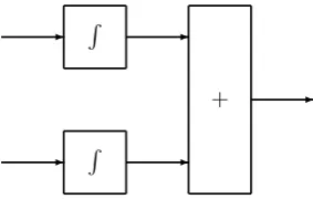
[image:29.595.224.366.494.584.2]As outlined inSection 3.4.1, analogue computers operate in real-time. This real-time behaviour permits analogue computers to achieve greater parallelism than their digital counterparts.
Figure 3.1shows a block diagram of a sample analogue computer. This computer integrates its two inputs and adds the two resultant signals to gen-erate the output. In this computer, the results would be outputted from both integrators simultaneously. Nevertheless, two identical integrators in digital hardware would also work in this way. However, the subsequent addition will happen in effectively zero time since its output will be generated concurrently with the outputs of the integrators. In other words, the adder will instanta-neously add the outputs of the integrators. To recapitulate, the two integra-tions and the addition are performed in parallel. In contrast, digital hardware would typically perform the integrations first, with the addition performed subsequently, leading to theoretically greater delays.
R
R
+
-Figure 3.1: Parallelism in analogue computers
Chapter 3. Analogue Computers 15
To summarise, in an analogue computer the propagation delay is effectively zero, irrespective of the complexity of its function. This is the greatest advan-tage offered by analogue computers.
3.4.3
Potentially Infinite Accuracy
Digital computers represent numbers using a finite number of bits. Conse-quently, digital signals always have a certain finite granularity or resolution. The only way to increase this resolution is to increase the word length, which is essentially the standard number of bits used to represent an entity in a partic-ular architecture, thereby consuming more die area and making the integrated circuits more expensive to manufacture. This finite granularity is clearly a problem since manufacturers are continually attempting to increase the word length of their CPUs, as evidenced by the recent migration of both the IBM PowerPC and Intel 80x86 architectures from 32 to 64 bits.
This has led to the formation of the study of numerical analysis or nu-merical methods. It involves reformulating mathematical problems in order to avoid truncation and rounding errors resulting from this finite number of bits. Such solutions only slightly improve accuracy and do not work in all sit-uations. This represents a problem. As Stoer and Bulirsch state, “Assessing the accuracy of the results of calculations is a paramount goal” [22, p. 1]. It would be advantageous if these problems could be completely disregarded.
Analogue computers represent numbers using continuous signals, with a potentially infinite range of values. Consequently, analogue computers do not suffer from any granularity problem. Therefore, the problems associated with digital may essentially be completely disregarded. This has resulted in com-puter theorists referring to analogue comcom-puters as real comcom-puters, which op-erate on the set of real numbers.
In summation, digital computers represent entities using an approximation while analogue computers represent entities using analogues to those entities.
3.5
Disadvantages
Analogue computers are rare today. This indicates that analogue computers have disadvantages. The main issues are noise, inflexibility and that they are not dynamically reconfigurable. This section discusses each of these in turn and highlights how they are unproblematic for the project’s physics engine.
3.5.1
Noise
Theoretical analogue computers offer infinite accuracy (Section 3.4.3). How-ever, practical analogue computers cannot realise this ideal.
Chapter 3. Analogue Computers 16
the nearest permissible voltage. Furthermore, adding error detection and cor-rection circuits to digital computers is unproblematic, but adding such circuits to analogue computers is relatively difficult.
There are, however, various techniques for reducing noise in analogue com-puters. The most successful technique is to use higher quality and, conse-quently, more expensive components. Additionally, there are a number of de-sign rules that attempt to reduce noise. One such dede-sign rule is specified in Section 6.6.5.
As outlined in Section 2.4.2, the primary application for the project’s physics engine is computer games. High accuracy is unimportant for games. Objects must only appear realistic; their behaviour does not need to be entirely accurate. In the project’s physics engine, any deviations were, as predicted, well within the limits of human perception. Therefore, for this physics engine, noise was almost completely disregarded.
3.5.2
Inflexibility
Analogue computers are inflexible in that they are limited in the variety of functions that they can perform. For computation on an analogue computer, a program must have a mathematical basis. In comparison, digital computers only require programs to have a Boolean algebraic basis, substantially increas-ing the variety of programs that can be created. For example, a program based on string manipulation could be expressed in Boolean algebra, but not in tra-ditional mathematics. This inflexibility was one of the principal reasons why analogue computers have decreased in popularity.
Physics is based on mathematics. Therefore, the inflexibility of analogue computers did not restrict the project’s physics engine. If additional functional-ity were desired, the digital circuits of hybrid computers could be used to sup-plement the capabilities of analogue computers, as discussed inSection 4.4.2.
3.5.3
Not Dynamically Reconfigurable
Traditional analogue computers cannot be dynamically reconfigured. Instead, their components are wired by hand for each objective. Wiring involves con-necting the necessary components together through a “patch-board” or “patch panel” consisting of terminals, similar to manually operated telephone ex-changes. Sophisticated analogue computers had detachable patch-boards that could be removed from the “patch bay” and later replaced, similar to the way programs can be saved on a digital computer.
Chapter 4
Hybrid Computers
Firstly, an overview of hybrid computers is presented. Next, their history is depicted before their traditional application domain is described. Finally, the advantages and disadvantages of hybrid computers are discussed.
This chapter’s objective is to provide the reader with an introduction to hybrid computers. Their history provides an insight into the different hybridi-sation concepts proposed. Disadvantages are outlined so that their influence on the project’s physics engine may be analysed.
4.1
Overview
A hybrid computer is a computer that consists of analogue and digital compu-tational elements. There is a cornucopia of definitions describing what exactly constitutes a hybrid computer, but for the purposes of this report, a hybrid computer is defined to be an analogue computer making use of some digital components.
The construction of such a system is not trivial, since analogue and digital are extremely dissimilar. The outputs generated by analogue components are continuous, while the outputs generated by digital components are discontin-uous.
4.2
History
The first hybrid systems constructed consisted of an existing analogue com-puter connected to an existing digital comcom-puter. They were not entirely new systems but the interconnection of two readily available systems.
The expansion of the US intercontinental ballistic missile (ICBM) pro-gramme in 1954, followed by the space race of the 1960s demanded greater computational power. Greater computational power meant that both analogue computers and their programs would substantially increase in size, making programming difficult and error-prone [17, p. 239]. Hybrid computers were proposed as the solution.
Convair Astronautics designed the first hybrid system in 1954, to perform simulation studies for the Atlas ICBM [15, p. 13]. It consisted of an Electronic
Chapter 4. Hybrid Computers 18
Associates, Inc (EAI) PACE analogue computer connected to an IBM 704 digital computer, via a converter called an Add-a-Verter manufactured by Epsco, Inc. In 1955, Ramo-Wooldridge Corporation developed a second hybrid system, for the same purpose as Convair’s. It also used an Add-a-Verter and a PACE analogue computer, but used a UNIVAC 1103A for its digital computation.
Commercially available computers typically used designs that were more primitive. For example, the HYDAC 2000 added some digital control elements to an analogue computer. It was much later before more sophisticated designs became available.
Despite the quantity of hybrid computers constructed, there was often dis-agreement as to the best way to unite analogue and digital, leading to a multi-tude of esoteric designs. For example, the TRICE system designed by Packard Bell for NASA’s spaceflight simulations used a pulse frequency modulated sig-nal as the information carrier, whereas most used conventiosig-nal sigsig-nals [18, p. 59].
Hybrid computers declined around the late 1970s during the demise of ana-logue computers (Section 3.2). After anaana-logue computers were deemed obso-lete, many believed the analogue component of the hybrid computer was a hindrance and that a digital computer was a better investment. Furthermore, it became increasingly obvious that hybrid computers were losing their niche as the abilities of digital computers improved [17, p. 264].
4.3
Applications
Hybrid computers can potentially be used where either analogue or digital computers are used. However, they were typically used for simulations that needed to model elements too complex for pure analogue computers. In par-ticular, hybrid computers were often used for scientific applications, in contrast to pure analogue computers, which were often used only for engineering ap-plications.
For example, Professor Vincent Rideout from the University of Wisconsin, in associated with NASA, modelled the cardiovascular respiratory system of the human body in 1972 [23, pp. 10–12]. This simulation used 120 differential equations to simulate the human heart, circulatory system, lungs and control systems.
4.4
Advantages
The advantages associated with hybrid computers are their ease of reconfig-urability and the way they unite the advantages of analogue and digital. These advantages are outlined below.
4.4.1
Reconfigurability
Chapter 4. Hybrid Computers 19
Digitally controlled analogue routing elements can be created to dynam-ically route analogue signals. Therefore, for increased flexibility, the control signals for these elements can originate from additional digital computing el-ements. Instead of manually wiring the computer, programs may be written that automatically reconfigure the computer. Such solutions alleviate the dif-ficulty of manually programming an analogue computer. Indeed, one of the motivating factors in the development of hybrid computers was the increasing complexity of analogue computers and the laboriousness of interconnecting their components.
Hybrid solutions impart the propensity to conceive reconfigurable ana-logue computers. This is the catalyst that made the project’s physics engine viable.
4.4.2
Leveraging Analogue and Digital
As outlined inSection 3.5.2, analogue computers have the ability to solve only a subset of the problems solvable on digital computers. However, as outlined inSection 3.4, analogue computers have certain advantages over their digital counterparts.
Hybrid computers can be constructed with analogue and digital partitions of equal status. Then, all functions that can be performed on an analogue com-puter would be performed using the analogue components. All other neces-sary functions would be performed using the digital components. This would allow for the computation of all functions that can be performed using a digital computer while leveraging the unique properties of analogue computers.
Hybrid computers offer a substantial increase in ability over analogue com-puters. However, it transpired that this functionality was not required by the project’s physics engine.
4.5
Disadvantages
Although hybrid computers solve many of the issues arising from analogue computers, the problem of noise remains partially unsolved. This issue is ex-amined below.
4.5.1
Noise
The analogue components in a hybrid computer will suffer from noise. More-over, since results generated by these analogue components will be used by digital components, the digital components will also essentially be affected by noise. A more thorough analysis of noise is provided inSection 3.5.1.
Chapter 5
Analogue
The primary objective of this chapter is to outline how analogue is still widely used today, despite advances in digital technology.
5.1
Overview
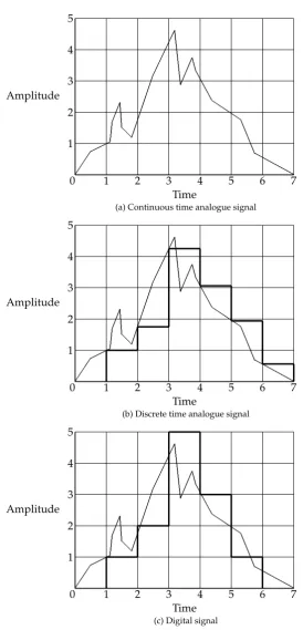
Analogue signals are defined over a continuous range of amplitudes. Typically, they are defined over a continuous range of times, as illustrated inFigure 5.1a. However, in ICs analogue signals are often defined only at discrete time values, as illustrated inFigure 5.1b[24, p. 2]. These are referred to as discrete time or sampled data analogue signals.
In contrast, digital signals are defined only at discrete times and discrete amplitudes, as illustrated inFigure 5.1c. They represent objects using only two values, zero and one.
Since digital is discrete in both time and amplitude, continuous analogue signals potentially allow for more accurate modelling of many objects. The properties of objects rarely have a finite number of levels but an infinite num-ber.
5.2
Applications
Many believe analogue is obsolete, having been superseded by digital. The proliferation of digital computers, digital television, digital cinema, digital ra-dio, digital music, digital cameras, digital camcorders and digital mobile tele-phony reinforces this viewpoint. However, this belief is unfounded.
There are many applications where analogue is still regularly used. Some of these applications are discussed below.
5.2.1
Wireless Communications
Today, there is substantial enthusiasm for wireless communications and this enthusiasm is constantly growing. Mobile telephones, wireless local area net-works (LANs) and wireless broadband all illustrate this trend.
Chapter 5. Analogue 21
Amplitude
Time
1 2 3 4 5 6 7
1 2 3 4 5
0
(a) Continuous time analogue signal
Amplitude
Time
1 2 3 4 5 6 7
1 2 3 4 5
0
(b) Discrete time analogue signal
Amplitude
Time
1 2 3 4 5 6 7
1 2 3 4 5
0
[image:36.595.128.403.114.685.2](c) Digital signal
Chapter 5. Analogue 22
The signals used for wireless communications are often transmitted close to the 1 GHz frequency range with only a few millivolts of amplitude. They will incur substantial noise during transmission. Therefore, a wireless receiver must amplify the appropriate part of the signal and filter out noise before processing, while operating at a very high speed. This can only be performed in analogue electronics, even for digital communications.
Therefore, these wireless devices typically must include both digital and analogue circuits on the same IC. This has led to a growth of interest in mixed-signal design. New languages have been proposed in order to simplify design, while tools allow for a more automated design flow. This is discussed further inSection 7.1.
5.2.2
Wireline Communications
Broadband technologies such as digital subscriber line (DSL) and cable broad-band are analogue-based. These technologies use multiple voltage levels, as opposed to only two digital levels. For example, four levels could be used, sending two merged bits simultaneously. This reduces the bandwidth re-quired. Additionally, to reduce the effects of attenuation and noise, signals are often modulated onto a carrier wave. Both of these techniques result in a conversion of the digital signal to an equivalent analogue one.
However, technologies with a digital basis such as LANs and fibre optic also use analogue processing techniques. In the case of communication over a fibre optic channel, the transmission is made using a laser diode, while the received signal is observed by a photodiode. Both devices are analogue in na-ture. Moreover, additional analogue processing must be performed to amplify the signal before conversion to digital.
5.2.3
Sensors
Sensors are also inherently analogue in nature. This applies for mechanical, electrical, acoustic and optical sensors. For example, the phototransistors in a digital camera produce analogue signals, which are only converted to digi-tal at a later processing step. A different type of sensor is used to control the airbag release mechanism in vehicles [25, pp. 4–5]. This uses a specially con-structed capacitor, which detects the sudden change in velocity indicating that the airbag should be released.
Recent developments in very large scale integration (VLSI) design allow for the sensor’s analogue and digital processing elements to be placed on the same IC as the sensor. This increases the level of mixed signal integration, fuelling the need for greater automation of analogue design.
5.2.4
Disk Drives
Chapter 5. Analogue 23
5.2.5
Microprocessors and Memories
Microprocessors and memories are digital. However, analogue issues arise in the design of these devices. For example, analysis of the distribution of high speed signals requires these signals to be treated as if they were analogue. Non-idealities in the device such as parasitic resistances and capacitances require knowledge of analogue design. In addition, the high speed sense amplifiers in memories are analogue circuits. Based on this, Razavi claims that “High-speed digital design is in fact analog design.” [25, p. 5]
5.2.6
Game Controllers
A game controller is a device used to control a computer game. They were originally entirely digital devices, but they are gradually gaining more ana-logue components.
Joysticks were the first devices to see this transition. Digital joysticks typ-ically had four or eight possible directions, corresponding to the compass points. In contrast, analogue joysticks have a much greater number of possi-ble directions and can determine the force with which they are being directed. However, there are a finite number of possible directions as the analogue out-put of the joystick is later converted to digital.
Buttons on game controllers are also making the transition to analogue. Pre-viously, buttons were either fully depressed or unpressed. Analogue buttons, in contrast, can determine the level to which they are depressed.
By transitioning game controllers to analogue, game developers are em-powered to make more immersive computer games that respond more pre-cisely to the user’s wishes.
5.2.7
Zoom
Chapter 6
Operational Amplifiers
This chapter provides an overview of operational amplifiers, which are the core elements of the analogue computer constructed as part of the project’s physics engine. Operational amplifier characteristics are briefly summarised before key operational amplifier circuits are demonstrated.
6.1
Overview
The operational amplifier or “op amp” is the core component of analogue com-puters. The operational amplifier is an amplifier with a very high open loop gain and a very low output impedance. It can be wired up with auxiliary pas-sive components, which cause the operational amplifier to perform a specific mathematical function. The relation of the output signal to the input signal is determined solely by the arrangement and magnitude of the other circuit elements.
6.2
History
In the early 1940s, George A Philbrick developed the first operational ampli-fier using vacuum tubes [26, p. 541]. Later, in 1962, Burr-Brown Corp and GAP/R developed the first IC-based operational amplifiers. However, in 1963, Fairchild Semiconductor’sµA702 became the first commercially available IC-based operational amplifier.
The best selling operational amplifier of all time is the 741. It was the first internally compensated operational amplifier available, meaning it required no external compensatory components. Released in 1968, it was invented by Dave Fullagar while working at Fairchild Semiconductor. The 741 is still manufac-tured by a number of companies, including National Semiconductor [27] and Texas Instruments [28], and has remained popular to this day. However, many operational amplifiers have since surpassed the 741’s characteristics, exploiting developments in semiconductor fabrication technologies.
Immediately following their introduction, operational amplifiers were a commercial success. In fact, they proved so popular that the commonly ac-cepted analogue design rules were reformulated to accommodate these
Chapter 6. Operational Amplifiers 25
vices. Their success is largely attributable to the availability of high perfor-mance amplifiers in discrete component form [29, p. 2]. To a large extent, the intricacies of an operational amplifier do not need to be comprehended. As a result, they may be treated as a black box, greatly simplifying circuit design.
6.3
Terminals
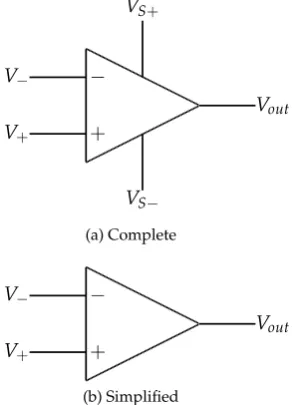
An operational amplifier typically has five terminals, as shown inFigure 6.1a:
V+ noninverting input
V− inverting input
Vout output
VS+ positive power supply
VS− negative power supply
VS+andVS−must always be connected to appropriate power supplies, typ-ically+15 V and−15 V. Therefore, circuit schematics usually eliminate these terminals, creating the circuit symbol depicted inFigure 6.1b. For all practical purposes,V−will be connected to ground.
Vout V−
V+
VS− VS+
+
−
(a) Complete
Vout V−
V+ +
−
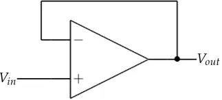
[image:40.595.231.381.391.594.2](b) Simplified
Figure 6.1: Operational amplifier circuit symbols
V− andVoutare used to control the mathematical operation performed by the operational amplifier. One component is typically placed in front of V−. Another is placed on the feedback loop created by connectingV−toVout. Such a configuration is illustrated inFigure 6.2.
Chapter 6. Operational Amplifiers 26
Vin
Vout
• •
+
−
Figure 6.2: Typical operational amplifier configuration. The boxes illustrate where circuit elements may be inserted.
6.4
Ideal Operational Amplifier
An ideal operational amplifier exhibits five main characteristics [29, p. 3]:
Infinite open loop gain The amplification from input to output with no feed-back applied is infinite. This makes the performance entirely dependent on input and feedback networks.
Infinite input impedance The impedance viewed from the two input termi-nals is infinite. This means that no current will flow in or out of either input terminal.
Infinite bandwidth The bandwidth range extends from zero to infinity. This ensures zero response time, no phase change with frequency and a re-sponse to direct current (DC) signals.
Zero output impedance The impedance viewed from the output terminal with respect to ground is zero. This ensures that the amplifier produces the same output voltage irrespective of the current drawn into the load.
Zero voltage and current offset This guarantees that when the input signal voltage is zero the output signal will also be zero, regardless of the in-put source impedance.
These characteristics imply a number of useful properties that may be ex-ploited when constructing operational amplifier circuits [21, pp. 9–12]:
Differential input An operational amplifier has a differential input. In other words, it only responds to the difference betweenV+ andV−. The value
ofV+−V−is essentially the input signal of the operational amplifier.
AC and DC An operational amplifier can process both alternating current (AC) and DC signals.
Chapter 6. Operational Amplifiers 27
6.5
Practical Operational Amplifier
The practical operational amplifier closely approximates the behaviour of the ideal operational amplifier. It deviates from the ideal in a number of details. Most of these may effectively be ignored and the analogue circuit designer can treat the operational amplifier as a black box. However, some of these details have an impact on the design of the project’s physics engine and must be considered. The most relevant of these are:
Finite bandwidth The range of frequency that may be inputted to the opera-tional amplifier is limited. This partially limits the range of signals that may be processed by the project’s physics engine.
Finite open loop gain The maximum amplification provided by the opera-tional amplifier is limited by the magnitude of the supply voltages. This results in upper and lower bounds being placed on the voltages that may be processed by the project’s physics engine.
In addition, it must be noted that some values of passive components will not work in the fashion suggested by the black box model. The values of these components must be within certain ranges if their behaviour is to coincide with that required by the operational amplifier.
Another deviation from ideality is that operational amplifiers typically have a voltage offset. Even when their inputs are zero they generate a small output voltage, which changes over time. This problem is easily overcome as many operational amplifiers include terminals to tune the amplifier.
6.6
Circuits
A vast number of circuits may be constructing using an operational amplifier at their core. The operational amplifier circuits relevant to the project’s physics engine are described below.
6.6.1
Inverter
The inverter is the basic operational amplifier configuration. This circuit can be constructed by placing a resistor at the V− input and another resistor on the feedback loop of an operational amplifier, as illustrated inFigure 6.3. The mathematical function performed by the circuit is:
Vout=−Vin
Rf
Rin
where
Vout = Voltage atVoutterminal Vin = Voltage atVinterminal
Chapter 6. Operational Amplifiers 28
Vin
Vout Rin
• •
+
−
[image:43.595.197.418.446.653.2]Rf
Figure 6.3: Inverter
6.6.2
Multiplier and Divider
By choosing the values ofRf andRin appropriately, the inverter circuit (Sec-tion 6.6.1) may be used to perform multiplica(Sec-tion or division b
![Table 2.1: Costs arising from implementing in-house physics software [12, p.23]](https://thumb-us.123doks.com/thumbv2/123dok_us/902333.602719/24.595.212.382.197.250/table-costs-arising-implementing-house-physics-software-p.webp)