University of Warwick institutional repository: http://go.warwick.ac.uk/wrap
A Thesis Submitted for the Degree of PhD at the University of Warwick
http://go.warwick.ac.uk/wrap/60439
This thesis is made available online and is protected by original copyright. Please scroll down to view the document itself.
012ÿ4567488ÿ
ÿ ÿ
ÿ
ÿ
ÿ
ÿ
ÿ
ÿ
8ÿ !"ÿ!#ÿ
$%&'(&ÿ*+,-%&.&ÿ./&ÿ0+%%+12345ÿ
6788ÿ:;<=>ÿ???????????????????????????????????@ÿ
A:BC=DEBFGÿHIÿ:7<J=D>ÿ??????????????????????????????ÿ
ÿ ÿ
7ÿ K!#ÿ!LM#ÿ
78ÿÿNÿOPQRSTUVPQÿUWVUÿOPQRSÿXYÿSRZ[TUSVU[\PÿVUÿUWRÿ]P[^RST[UY_ÿNÿVXÿSR`O[SRQÿU\ÿQRa\T[UÿXYÿUWRT[Tÿb[UWÿUWRÿ ]P[^RST[UYÿ[Pÿcde1ÿWVSQÿf\aYÿVPQÿ[PÿQ[Z[UVgÿh\SXVUÿeWRÿQ[Z[UVgÿ^RST[\PÿTW\OgQÿP\SXVggYÿiRÿTV^RQÿVTÿVÿ T[PZgRÿaQhÿh[gRÿ
ÿ
77ÿÿeWRÿWVSQÿf\aYÿb[ggÿiRÿW\OTRQÿ[PÿUWRÿ]P[^RST[UYÿj[iSVSYÿeWRÿQ[Z[UVgÿ^RST[\Pÿb[ggÿiRÿQRa\T[URQÿ[PÿUWRÿ A:BC=DEBFGkEÿH:EFBF7FBl:;8ÿm=nlEBFlDGÿopqrstÿ]PgRTTÿ\UWRSb[TRÿ[PQ[fVURQÿoTRRÿ7uÿiRg\btÿUW[Tÿb[ggÿiRÿXVQRÿ \aRPgYÿVffRTT[igRÿ\PÿUWRÿNPURSPRUÿVPQÿb[ggÿiRÿTOaag[RQÿU\ÿUWRÿcS[U[TWÿj[iSVSYÿU\ÿiRÿXVQRÿV^V[gVigRÿ\Pg[PRÿ^[Vÿ [UTÿvgRfUS\P[fÿeWRTRTÿdPg[PRÿwRS^[fRÿoveWdwtÿTRS^[fRÿ
xrUÿaSRTRPU_ÿUWRE=EÿE7J<BFF=yÿzlDÿ;ÿ{;EF=DkEÿy=|D==ÿJGÿm=E=;D}~ÿ{ÿ{}ÿ{ÿ{ÿlDÿ{{=y}BÿVSRÿ P\UÿiR[PZÿQRa\T[URQÿ[PÿpqrsÿVPQÿP\UÿiR[PZÿXVQRÿV^V[gVigRÿ^[VÿvUWdwÿeW[TÿXVYÿfWVPZRÿ[PÿhOUOSR ÿ ÿ
7uÿÿNPÿRfRaU[\PVgÿf[SfOXTUVPfRT_ÿUWRÿWV[Sÿ\hÿUWRÿc\VSQÿ\hÿ2SVQOVURÿwUOQ[RTÿXVYÿZSVPUÿaRSX[TT[\Pÿh\Sÿ VPÿRXiVSZ\ÿU\ÿiRÿagVfRQÿ\PÿaOig[fÿVffRTTÿU\ÿUWRÿWVSQÿf\aYÿUWRT[Tÿh\SÿVÿg[X[URQÿaRS[\QÿNUÿ[TÿVgT\ÿa\TT[igRÿU\ÿ VaagYÿTRaVSVURgYÿh\SÿVPÿRXiVSZ\ÿ\PÿUWRÿQ[Z[UVgÿ^RST[\Pÿo6OSUWRSÿ[Ph\SXVU[\Pÿ[TÿV^V[gVigRÿ[PÿUWRÿ2&ÿ.+ÿ ',23'.2+3(ÿ0+ÿ24/&ÿ&4&&(ÿÿ&(&'*/tÿ
ÿ
7ÿÿÿÿÿ ¡ ¢£ÿÿ¡¤ ÿÿÿ¥¡¦ÿ£ÿ§ÿ¨©¤ªÿ«ÿ©¬«¡ÿ©¡ ¢ÿ®ÿ§«¯°ÿ ±+ÿ'%%ÿ+./&ÿ&(&'*/ÿ&4&&(²ÿ-%&'(&ÿ*+,-%&.&ÿ+./ÿ(&*.2+3(ÿ³'´ÿ'3ÿ³´ÿ&%+15ÿ
ÿ
oVtÿ 1VSQÿ\aYÿ ÿ
NÿWRSRiYÿQRa\T[UÿVÿWVSQÿf\aYÿ\hÿXYÿUWRT[Tÿ[PÿUWRÿ]P[^RST[UYÿj[iSVSYÿU\ÿiRÿXVQRÿaOig[fgYÿV^V[gVigRÿU\ÿ SRVQRSTÿoagRVTRÿQRgRURÿVTÿVaaS\aS[VURtÿvNe1vqÿ[XXRQ[VURgYÿdqÿVhURSÿVPÿRXiVSZ\ÿaRS[\Qÿ\hÿ ???@@@@@@@@@@@@@@ÿX\PUWT6YRVSTÿVTÿVZSRRQÿiYÿUWRÿWV[Sÿ\hÿUWRÿc\VSQÿ\hÿ2SVQOVURÿwUOQ[RTÿÿ ÿ
NÿVZSRRÿUWVUÿXYÿUWRT[TÿXVYÿiRÿaW\U\f\a[RQÿ ÿ ÿÿÿÿÿÿµvwÿ6ÿ¶dÿo$%&'(&ÿ&%&.&ÿ'(ÿ'--+-2'.&tÿ
ÿ
oitÿ ¸[Z[UVgÿ\aYÿ ÿ
NÿWRSRiYÿQRa\T[UÿVÿQ[Z[UVgÿf\aYÿ\hÿXYÿUWRT[TÿU\ÿiRÿWRgQÿ[PÿpqrsÿVPQÿXVQRÿV^V[gVigRÿ^[VÿveWdwÿÿ ÿ
sgRVTRÿfW\\TRÿ\PRÿ\hÿUWRÿh\gg\b[PZÿ\aU[\PT¹ÿ ÿ
vNe1vqÿÿÿºYÿUWRT[TÿfVPÿiRÿXVQRÿaOig[fgYÿV^V[gVigRÿ\Pg[PRÿÿÿÿÿÿµvwÿ6ÿ¶dÿo$%&'(&ÿ&%&.&ÿ'(ÿ'--+-2'.&tÿ
ÿ
dqÿÿÿºYÿUWRT[TÿfVPÿiRÿXVQRÿaOig[fgYÿV^V[gVigRÿ\PgYÿVhURS?@@»QVUR ÿÿosgRVTRÿZ[^RÿQVURtÿ
ÿ ÿ ÿ ÿ ÿ ÿ ÿ ÿÿÿÿÿÿÿÿÿµvwÿ6ÿ¶dÿo$%&'(&ÿ&%&.&ÿ'(ÿ'--+-2'.&tÿ ÿ
dqÿÿÿºYÿhOggÿUWRT[TÿfVPP\UÿiRÿXVQRÿaOig[fgYÿV^V[gVigRÿ\Pg[PRÿiOUÿNÿVXÿTOiX[UU[PZÿVÿÿÿTRaVSVURgYÿ [QRPU[h[RQÿÿÿVQQ[U[\PVg_ÿViS[QZRQÿ^RST[\PÿUWVUÿfVPÿiRÿXVQRÿV^V[gVigRÿ\Pg[PRÿ
ÿÿÿÿÿÿÿÿÿÿµvwÿ6ÿ¶dÿo$%&'(&ÿ&%&.&ÿ'(ÿ'--+-2'.&tÿ ÿ
dqÿÿÿºYÿUWRT[TÿfVPP\UÿiRÿXVQRÿaOig[fgYÿV^V[gVigRÿ\Pg[PRÿÿÿÿÿÿÿÿÿÿµvwÿ6ÿ¶dÿo$%&'(&ÿ&%&.&ÿ'(ÿ'--+-2'.&tÿ
ÿ ÿ ÿ
¼½¾¿ÀÁÿÃÀ¿ÄÁÿÅÁƾ¾Ç ÈÉÈÊËÌÍ
ÎÎÎÎÎÎÎÎÎÎ ÎÎÎÎÎÎÎÎÎÎÎÎÎÎÎÎÎÎÎÎÎÎÎÎÎÎÎÎÎÎÎÎÎÎÎÎÎÎ
ÎÎÎÎÎ
ÎÎÎÎÎÎÎÎÎÎÎÎÎÎÎÎÎÎÎÎÎÎÎÎÎÎÎÎÎÎÎÎÎÎÎÎÎÎÎÎÎÎÎÎÎÎÎÎÎÎÎÎÎÎÎÎÎÎÎÎÎÎÎÎÎÎÎÎÎÎÎÎÎÎÎÎÎÎÎÎÎÎÎÎÎÎ ÎÎÎÎÎÎÎÎÎÎÎÎÎÎÎÎÎÎÎÎÎÎÎÎÎÎÎÎÎÎÎÎÎÎÎÎÎÎÎÎ
ÎÎÎÎÎÎÎÎÎÎÎÎÎÎÎÎÎÎÎÎÎÎÎÎÎÎÎÎÎÎÎÎÎÎÎÎÎÎÎÎÎÎÎÎÎÎÎÎÎÎÎÎÎÎÎÎÎÎÎÎÎÎÎÎÎÎÎÎÎÎÎÎÎÎÎÎÎÎÎÎÎ ÎÎÎÎ
ÎÎÎÎÎÎÎÎÎÎÎÎÎÎÎÎÎÎÎÎÎÎÎÎÎÎÎÎÎÎÎÎÎÎÎÎÎÎÎÎÎÎÎÎÎÎÎÎÎÎÎÎÎÎÎÎÎÎÎÎÎÎÎÎÎÎÎÎÎÎÎÎÎÎÎÎÎÎÎÎÎÎÎÎÎÎÎÎÎÎÎÎÎÎÎÎÎÎÎÎÎÎÎÎÎÎÎÎÎÎÎÎÎ
ÎÎÎÎÎÎÎÎÎÎÎÎÎÎÎÎÎÎÎÎÎÎÎÎÎÎÎÎÎÎÎÎÎÎÎÎÎÎÎÎÎÎÎÎÎÎÎÎÎÎÎÎÎÎÎÎÎÎÎÎÎÎÎÎÎÎÎÎÎÎ
ÎÎÎÎÎÎÎÎÎÎÎÎÎÎÎÎÎÎÎÎÎÎÎÎÎÎÎÎÎÎÎÎÎÎÎÎÎÎÎÎÎÎÎÎÎÎÎÎÎÎÎÎÎÎÎÎÎÎÎÎÎÎÎÎÎÎÎÎÎÎÎÎÎÎÎÎÎÎÎÎÎÎÎÎÎÎÎÎÎ ÎÎÎÎ
thomas j. osgood
SEMANTIC LABELLING OF ROAD SCENES USING SUPERVISED AND UNSUPERVISED MACHINE LEARNING WITH LIDAR-STEREO SENSOR
FUSION
thesis
Submitted to the University of Warwick
for the degree of
doctor of philosophy
SEMANTIC L ABELLING OF ROAD SCENES USING
SUPERVISED AND UNSUPERVISED MACHINE LEARNING
WITH LIDAR-STEREO SENSOR FUSION
thomas j. osgo od
thesis
Submitted to the University of Warwick
for the degree of
d o ctor of philosophy
International Manufacturing Centre
Thomas J. Osgood:Semantic labelling of road scenes using supervised and unsupervised machine learning with LIDAR-stereo sensor fusion,Primarily for the improvement of
All of the biggest technological inventions created by man - the air plane, the auto mobile, the computer - says little about his intelligence, but speaks volumes about his laziness.
C ONTENT S
Acknowledgements xvii
Declaration xviii
Publications xix
Abstract xx
Acronyms xxi
1 introduction 1
1.1 Advanced driver assistance systems (ADAS) 1
1.2 Basic concepts 5
1.2.1 Semantic labelling 5
1.2.2 Stereo vision 6
1.2.3 LIDAR 8
1.2.4 Supervised learning 11
1.2.5 Unsupervised learning 12
1.3 Aims and contributions of thesis 12
1.4 Thesis outline 15
2 literature review 19
2.1 Depth from stereo 19
2.1.1 Image capture, preparation and pre-processing 20
2.1.2 Feature matching 23
2.1.3 Verification of matching 27
2.1.4 Distance calculation 28
2.2 LIDAR to camera calibration 30
contents viii
2.3 Machine learning 31
2.3.1 Artificial neural networks 31
2.3.2 Support vector machines 34
2.3.3 K-means clustering for unsupervised learning 36
2.4 Image processing 38
2.4.1 Edge detection 38
2.4.2 Segmentation 40
2.5 General semantic classification 41
3 lidar calibration and fusion for improved depth maps 47
3.1 Calibration overview 48
3.2 Problem definition 49
3.3 Approach 52
3.3.1 Nelder-Mead algorithm 52
3.3.2 Definition of the objective function 53
3.4 Previous work to determine number of required targets 58
3.5 Collection of test data 61
3.6 Results and discussion 68
3.6.1 Calibration results 68
3.6.2 Validation of results using initial conditions 70
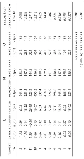
3.6.3 Validation using independent samples 72
3.7 Fusion and merging of sensor data 72
3.7.1 Final calibration 74
3.7.2 LIDAR interpolation 75
3.8 Theoretical stereo noise performance 79
4 data collection and set description 83
4.1 Data collection hardware 84
4.1.1 The ibeo LUX LIDAR 84
contents ix
4.1.3 Point Grey Research bumblebee2 87
4.1.4 Computer hardware 89
4.2 Notes on data collection 89
4.3 Data sets 95
4.3.1 The “A46” set 95
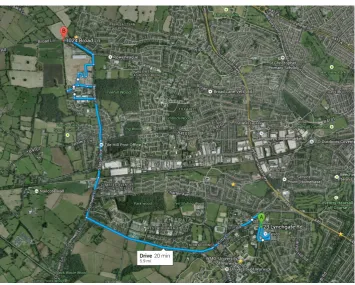
4.3.2 The “RX Residential” set 96
4.3.3 The “Berkswell Auto” set 97
4.3.4 The “Berkswell Manual” set 98
4.3.5 Sample images from the sets 99
5 image segmentation and analysis for training 101
5.1 Colour and contrast correction 102
5.2 Hybrid image segmentation 105
5.2.1 Step 1: Canny edge detection with region closing 107
5.2.2 Step 2: Depth map segmentation 111
5.2.3 Step 3: Mean-shift texture segmentation 114
5.2.4 Step 4: Segmentation fusion 116
5.2.5 Performance of segmentation fusion method 119
5.3 Choice of colour space representation 122
5.4 Texture and shape properties 128
5.5 Choice of depth augmented descriptors 138
5.5.1 Point cloud orientation 140
5.5.2 Point cloud planarity 143
5.6 Discriminatory analysis with principal component analysis 150
5.7 Conclusion 157
6 supervised learning with manually labelled images 159
6.1 Data preparation 160
6.1.1 Frame selection and manual labelling 160
contents x
6.2 Experiment setup 168
6.2.1 Support vector machine configuration 169
6.2.2 Neural network configuration 172
6.2.3 Comparison methodology 176
6.3 Training results 177
6.4 Conclusion 187
7 experiment with unsupervised learning 191
7.1 Experiment setup 194
7.2 Choosing the optimal number of sub-classes 196
7.3 Classification results 200
7.4 Conclusion 203
8 conclusions and further work 207
8.1 Key findings and contributions 208
8.1.1 LIDAR calibration 208
8.1.2 Data collection 210
8.1.3 Segmentation and segment analysis 212
8.1.4 Comparison of classifiers based on supervised learning 217
8.1.5 Evaluation of unsupervised classifier 219
8.2 Recommendations for further work 221
a appendix: video details and code listings 226
a.1 Video result description 226
a.2 Objective function of calibration chapter 229
a.3 Fusion segmentation 230
a.4 Plane orientation 232
LIST OF FIGURES
Figure 1.1 Example of semantic labelling 5
Figure 1.2 Stereo vision diagram 7
Figure 1.3 Basic principle of LIDAR distance measurement 9
Figure 1.4 The ibeo LUX LIDAR 10
Figure 1.5 Example of classification results 13
Figure 1.6 Data flow-chart and function contents page 16
Figure 2.1 Binocular stereo vision geometry 29
Figure 2.2 Artificial neural network diagram 33
Figure 2.3 Semantic labelling example from Posner et al. [148] 44
Figure 2.4 Semantic labelling example from Ess et al. [42] 45
Figure 3.1 Sensor fusion configuration 51
Figure 3.2 Results of preliminary Nelder-Mead calibration work 58
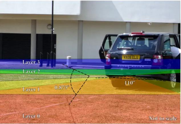
Figure 3.3 Target used for LIDAR calibration 61
Figure 3.4 Physical setup of the fusion system 62
Figure 3.5 Captured data from the camera and the laser scanner 63
Figure 3.6 Required target size at a given distance 64
Figure 3.7 Expected vertical position in the camera image 66
Figure 3.8 ibeo LUX scan layer diagram 67
Figure 3.9 Results of calibration with lens distortion model 70
Figure 3.10 Demonstration of calibrated sensor fusion data 71
Figure 3.11 Sensor mounting positions on data collection vehicle 76
Figure 3.12 LIDAR interpolation and range bound estimation 77
Figure 3.13 Improved stereo after integrating LIDAR depth information 78
List of Figures xii
Figure 3.14 Evaluation of LIDAR to stereo fusion accuracy 81
Figure 3.15 Histogram of error magnitude fromFigure 3.14. 82
Figure 4.1 Land Rover used for data collection 84
Figure 4.2 ibeo LUX four layer LIDAR 86
Figure 4.3 Videre STOC stereo on chip system 87
Figure 4.4 Point Grey Research Bumblebee2 88
Figure 4.5 HP EliteBook8540w 90
Figure 4.6 Example of image tearing due to insufficient processing power while using H264compression codec 93
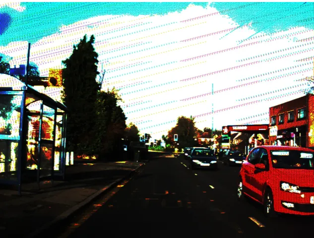
Figure 4.7 Example of decoder noise, contrast greatly enhanced 94
Figure 4.8 Map of route taken for dataset “A46” 95
Figure 4.9 Map of route taken for dataset “RX Residential” 96
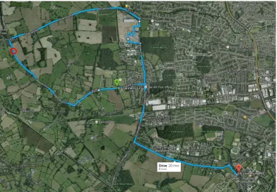
Figure 4.10 Map of route taken for dataset “Berkswell Auto” 97
Figure 4.11 Map of route taken for dataset “Berkswell Manual” 98
Figure 4.12 Sample of set “A46” 99
Figure 4.13 Sample of set “RX Residential” 99
Figure 4.14 Sample of set “Berkswell automatic” 100
Figure 4.15 Sample of set “Berkswell manual” 100
Figure 5.1 Example of ineffective contrast enhancement 103
Figure 5.2 Example of grey-world colour correction 104
Figure 5.3 Example of EDISON mean-shift segmentation 106
Figure 5.4 Demonstration of enhanced Canny segmentation 107
Figure 5.5 Illustration of Canny threshold levels 109
Figure 5.6 Secondary edge search for region closing 110
Figure 5.7 Example of binary morphology operations on test image 110
Figure 5.8 Example of closed region Canny edge detection 111
Figure 5.9 Example depth map to demonstrate depth segmentation 111
List of Figures xiii
Figure 5.11 Merging of depth segmentation with edge segmentation 114
Figure 5.12 Outputs from the three segmentation fusion steps 116
Figure 5.13 Merging of small regions from edge segmentation 118
Figure 5.14 Output of segmentation fusion on sample1 118
Figure 5.15 Output of segmentation fusion on sample2 119
Figure 5.16 Evaluation of segmentation performance 120
Figure 5.17 Example of RGB colour space 124
Figure 5.18 Example of HSV colour space 127
Figure 5.19 Sample image to demonstrate texture descriptors 128
Figure 5.20 Colour coded magnitude maps showing hue mean and hue STD 129
Figure 5.21 Colour coded magnitude maps showing saturation mean and saturation STD 129
Figure 5.22 Colour coded magnitude maps showing intensity mean and intensity STD 130
Figure 5.23 Colour coded magnitude maps showing intensity range and maximum intensity 131
Figure 5.24 Colour coded magnitude maps showing entropy and vertical position 132
Figure 5.25 Colour coded magnitude maps showing solidity and area of segments 133
Figure 5.26 Colour coded magnitude maps showing horizontal GLCM con-trast and correlation of segment 135
Figure 5.27 Colour coded magnitude maps showing horizontal GLCM ho-mogeneity and energy 135
Figure 5.28 GLCM matrix analysis illustration 137
List of Figures xiv
Figure 5.30 Image and disparity map of road segment used to extract point cloud 139
Figure 5.31 Point cloud extracted from road segment 139
Figure 5.32 Linear surface fitted to road point cloud 142
Figure 5.33 Point cloud rotation and offset prior to polynomial surface fit-ting 144
Figure 5.34 Polynomial surface fitted to road point cloud 147
Figure 5.35 Colour coded magnitude maps showing height and plane fit MSE 147
Figure 5.36 Example of robust plane fitting, MSE is less than0.001 149
Figure 5.37 Example of non-robust plane fitting, MSE is0.03 150
Figure 5.38 Box plot of segment measurement data 152
Figure 5.39 Variance explained by each principal component 154
Figure 5.40 1stand 2ndprincipal components 155
Figure 5.41 1stand 3rdprincipal components 156
Figure 6.1 Software used for manual image tagging 162
Figure 6.2 Deriving target class from pixel tagging 164
Figure 6.3 Class membership counts 166
Figure 6.4 Grid search for SVM parameters 171
Figure 6.5 Determining optimal number of hidden nodes 175
Figure 6.6 Confusion matrix for SVM classifier 179
Figure 6.7 Confusion matrix for neural network classifier 180
Figure 6.8 ROC curve for SVM classifier 181
Figure 6.9 ROC curve for neural network classifier 182
Figure 6.10 Confusion matrix for SVM classifier without “None” class 184
Figure 6.11 ROC curve for SVM classifier without “None” class 185
Figure 6.12 Classifier output example one 188
Figure 6.14 Classifier output example three 190
Figure 7.1 Example of sub-class to super-class mapping 193
Figure 7.2 Accuracy of unsupervised method against sub-class count 197
Figure 7.3 BRR of unsupervised method against sub-class count 198
Figure 7.4 Distribution of super-class membership against sub-class count 199
Figure 7.5 Confusion matrix for unsupervised classifier 201
Figure 7.6 Classifier output example four 204
Figure 7.7 Classifier output example five 205
LISTINGS
Listing 3.1 Optimisation report associated with the results inFigure 3.9 69
Listing A.1 Objective function of calibration optimisation,φ 229
Listing A.2 Segmentation fusion 230
Listing A.3 Plane orientation 232
LIST OF TABLES
Table 3.2 Initial values for calibration parameters 68
Table 3.3 Independent samples and resulting projection for calibration validation 73
Table 3.4 Final calibration parameters used during the acquisition of all datasets 75
Table 4.1 Video compression settings for data recording 94
Table 4.2 Summary of "A46" Dataset 95
Table 4.3 Summary of "RX Residential" Dataset 96
Table 4.4 Summary of "Berkswell Auto" Dataset 97
Table 4.5 Summary of "Berkswell Manual" Dataset 98
Table 5.1 Parameters used in EDISON package 115
Table 5.2 Summary of segmentation performance test 121
Table 6.1 Summary of classes and weightings 167
Table 6.2 Summary of classification results 186
Table 7.1 Summary of unsupervised classification results 203
If we knew what we were doing,
it wouldn’t be called research,
would it?
— Albert Einstein[76]
ACKNOWLED GEMENT S
It would not have been possible to write this doctoral thesis without the help and support of the numerous kind people around me both within, and outside of, the University of Warwick. It would be impossible to mention everyone who has been involved here, but the following people have been particularly influential and supportive over the4years
that I have been conducting this research.
Above all I would like to thank my partner Rui Xin and my parents for their unyielding efforts to keep me motivated and working despite my huge reluctance at times! Also my sister, Sally, for putting in all those hours of hand labelling of images for research purposes!
When it came to writing this thesis it would not have been possible without the constant enthusiasm and encouragement from my second supervisor Dr. Emma Rushforth and my initial secondary supervisor Prof. Ken Young who unfortunately could not see my PhD through to its conclusion.
On the academic side, I would like to thank my first supervisor Dr. Yingping Huang for his ideas and great experience in the field of image processing and all of his input during the early stages of the project. On this note I would also like to thank Dr. Thomas Popham and Anna Gaszczak whose contributions to the texture analysis work were invaluable. Finally I would like to gratefully acknowledge Alain Dunoyer and Paul Nichols from the Jaguar Land Rover group for their support throughout the research phases of this work by allowing access to their equipment.
DECL AR ATION
I confirm that the work presented in this thesis is entirely my own work, conducted under the supervision of Dr. Emma Rushforth. No part of the work contained in this thesis has been submitted for a degree at any other university.
Coventry, August 2013
PUBLICATIONS
Some ideas and figures have appeared previously in the following publications:
• Thomas J. Osgood, Yingping Huang, and K. Young. Minimisation of alignment error between a camera and a laser range finder using nelder-mead simplex direct search. In2010 IEEE Intelligent Vehicles Symposium (IV), pages 779–786. IEEE,
June 2010. ISBN 978-1-4244-7866-8. doi: 10.1109/IVS.2010.5548126
• Thomas J. Osgood and Yingping Huang. Sensor fusion calibration for driver asistance systems. In2011 IEEE International Conference on Vehicular Electronics and Safety (ICVES), pages 187–192. IEEE, July 2011. ISBN 978-1-4577-0576-2. doi:
10.1109/ICVES.2011.5983812
• Thomas J. Osgood and Yingping Huang. Calibration of laser scanner and camera fusion system for intelligent vehicles using Nelder–Mead optimization. Meas-urement Science and Technology, 24(3):035101, March 2013. ISSN 0957-0233,
1361-6501. doi: 10.1088/0957-0233/24/3/035101. URLhttp://iopscience.iop.org/ 0957-0233/24/3/035101
ABSTR ACT
At the highest level the aim of this thesis is to review and develop reliable and efficient algorithms for classifying road scenery primarily using vision based technology mounted on vehicles. The purpose of this technology is to enhance vehicle safety systems in order to prevent accidents which cause injuries to drivers and pedestrians.
This thesis uses LIDAR–stereo sensor fusion to analyse the scene in the path of the vehicle and apply semantic labels to the different content types within the images. It details every step of the process from raw sensor data to automatically labelled images.
At each stage of the process currently used methods are investigated and evaluated. In cases where existing methods do not produce satisfactory results improved methods have been suggested. In particular, this thesis presents a novel, automated, method for aligning LIDAR data to the stereo camera frame without the need for specialised alignment grids. For image segmentation a hybrid approach is presented, combining the strengths of both edge detection and mean-shift segmentation. For texture analysis the presented method uses GLCM metrics which allows texture information to be captured and summarised using only four feature descriptors compared to the100’s produced by SURF descriptors.
In addition to texture descriptors, the 3D information provided by the stereo system is also exploited. The segmented point cloud is used to determine orientation and curvature using polynomial surface fitting, a technique not yet applied to this application.
Regarding classification methods a comprehensive study was carried out comparing the performance of the SVM and neural network algorithms for this particular application. The outcome shows that for this particular set of learning features the SVM classifiers offer slightly better performance in the context of image and depth based classification which was not made clear in existing literature.
Finally a novel method of making unsupervised classifications is presented. Segments are automatically grouped into sub-classes which can then be mapped to more expressive super-classes as needed. Although the method in its current state does not yet match the performance of supervised methods it does produce usable classification results without the need for any training data. In addition, the method can be used to automatically sub-class classes with significant inter-class variation into more specialised groups prior to being used as training targets in a supervised method.
ACRONYMS
ADAS Advanced Driver Assistance Systems AGC Automatic Gain Control
ANN Artificial Neural Network BER Balanced Error Rate BRR Balanced Recall Rate
CCD Charge-Coupled Device
CMOS Complementary Metal-Oxide-Semiconductor
EDISON Edge Detection and Image Segmentation FOV Field Of View
FPGA Field-Programmable Gate Array GLCM Gray-Level Co-occurrence Matrix HSV Hue, Saturation, Value
JLR Jaguar Land Rover
LIDAR Light Detection And Ranging MSE Mean Squared Error
PCA Principal Component Analysis PnP Perspective-n-Point
RBF Radial Basis Function
RGB Red, Green, Blue
ROC Receiver Operating Characteristic
SRI Spherical Range Image STOC Stereo On Chip
SVD Singular Value Decomposition SVM Support Vector Machine
1
INTRODUCTION
c o n t e n t s
1.1 Advanced driver assistance systems (ADAS) 1 1.2 Basic concepts 5
1.2.1 Semantic labelling 5 1.2.2 Stereo vision 6
1.2.3 LIDAR 8
1.2.4 Supervised learning 11 1.2.5 Unsupervised learning 12 1.3 Aims and contributions of thesis 12 1.4 Thesis outline 15
1.1
advanced driver assistance systems ( adas)
Cars have become safer for their occupants in recent years due to passive safety features installed by most of the major motor manufacturers in the EEC. Because of this the chances of being seriously injured in a crash have diminished, however, with the recent surge in the number of road users the frequency of collisions continues to rise. More cars on the road means less room for driver error so, consequently, despite passive safety systems there has been little change in the number of collisions leading to personal injury. In fact recent road safety reports from the Department for Transport [53,178] show a small increase in driver casualties since2010in the UK.
1.1 advanced driver assistance systems (adas) 2
Passive systems such as air bags and crumple zones provide a reasonable level of protection to the driver and passengers after impact but, the only sure way of preventing road user injury (and damage to property) is to prevent collisions from occurring in the first place. While some accidents, such as mechanical failure, are truly beyond the driver’s control, the vast majority could be avoided if road vehicles had the ability to predict collisions and take evasive action. This is the principal aim of Advanced Driver Assistance Systems (ADAS)
- systems which assist the driver by detecting and correcting driver mistakes. Some examples ofADASsystems that already exist are lane departure warning systems and automatic parallel parking systems.
The idea for anADASwhich predicts and prevents collisions is not new, several research
groups are already building such systems at the time of writing (e.g. PreVent [180]). All
ADASsystems involve the interaction of many sub-systems from different engineering
disciplines including software, hardware and mechanical aspects, however the two most important components are:
1. The sensing of the area surrounding the vehicle: A vehicle that can predict colli-sions would need to have information about what is happening in its immediate surroundings, particularly regarding other vehicles, pedestrians, solid obstacles and even road signs. These data can be collected in various forms via sensors that already exist, or will soon exist on commercially available vehicles. The purpose of collecting and analysing the data is so that other projects, such as PreVent, can integrate them into systems which perform the second important step in the collision avoidanceADASbelow.
1.1 advanced driver assistance systems (adas) 3
physical intervention in the control of the vehicle including computer controlled brakes and steering override. This aspect of the system will not be covered in this thesis.
Going back to point1, there are a number of ways of collecting this information, using
several types of currently available sensor. When considering which sensors are suitable for this application the priority is to make a selection that can be easily and economically fitted to the majority of road vehicles. The performance of the sensors is the secondary consideration, at the moment, since it will be some time until 3D rotating Light Detec-tion And Ranging (LIDAR) devices, for example, can be fitted to every vehicle at a low
cost (presently even single planeLIDARdevices such as the LUX are in the region of
£14, 000[64]). However, history has shown us that new technologies quickly become
more affordable.
One good choice is to use video cameras – they are so cheap to produce now that some production vehicles, such as the new Land Rover line from Jaguar Land Rover (JLR), already come fitted with a set of cameras that capture a360◦view of the surroundings.
A single camera however can only provide the driver with the means to see behind the vehicle. A pair of cameras, on the other hand, can be used to estimate size, shape and distances using stereo techniques discussed in the next section. Ultra-sound devices are also fitted to the majority of modern cars to assist in parking and manoeuvring however, due to their extremely short range, they are not applicable to collision avoidance at normal driving speeds. The other choices for active distance sensing are radar andLIDAR. Since LIDARoutperforms radar in terms of accuracy and resolution it is generally favoured in
ADASresearch.
1.1 advanced driver assistance systems (adas) 4
nothing but a matrix of values. There is no information about the size, shape, distance and properties of any object seen in that image. On the other hand, the human eye can infer all that information and more just by looking at a single snapshot. The difference lies in the fact that humans can recognise the objects that compose the scene; they know how each of these objects behaves, what size it is, how fast it might be moving and whether it should be a cause for concern, if it appears in the path of the vehicle. In order to help computers determine the more difficult attributes, such as size, sensors such as stereo cameras andLIDARdevices can be used to reconstruct the scene in 3D allowing real world measurements to be made.
Vehicles capable of sensing their surroundings are not only of interest to car manufactures for safety systems, but the underlying systems are also applicable to autonomous space exploration e.g. the Mars rover [115], military applications e.g. the DARPA challenge [171] and fully autonomous passenger cars e.g. [120]. The ability to autonomously detect and avoid pedestrians, for example, would be the next step in the suite of existing vision based driver assistance technologies such as road sign detection (e.g. Broggi et al. [22]) and lane departure warning systems (e.g. McCall and Trivedi [117]).
1.2 basic concepts 5
Figure 1.1: Example of semantic labelling.
1.2
basic c oncep ts
1.2.1 Semantic labelling
Semantic labelling, also know as scene parsing or full screen labelling, is the process of identifying the content in every region of an image. The idea is partly inspired by the way a human perceives a road scene – the goal being to mimic this understanding and to separate the raw data into individual surface types that make up the surroundings. If this can be done, then the data from the sensors can become more than just data, they will become a description, or labelled map of the environment, which can easily be queried to decide, for example, if the space ahead is safe to drive in. So, in the same way that a human can look at an image and identify pedestrians, cars, trees, pavements etc. in the image, this data analysis system will attempt to identify the same regions of the image and label them as that object.
A simplified step-by-step description of this process would look like this:
1.2 basic concepts 6
b. Images will be processed to find edges and boundaries, this is known as segmenta-tion. Simplistically this would be done by detecting lines in the image that separate regions of different colour, or brightness.
c. For each of the segments identified in the previous step, take measurements and make observations on the content of the segment which might help identify what this region contains. This might include measurements such as the colour, the brightness and the texture of the image segment.
d. Supposing that one has some corpus of data which describes the relationship between these observations and what type of object they relate to, then: given all the information that has now been collected about each segment, the content can be identified, or matched, to a known type of object. As a simplified example, suppose it is known that segments that are mostly grey contain road, then any segments matching this description can be labelled as road. The more information that is available the more precise the prediction will be.
e. The result will be a labelled version of the original image and all the associated information these labels infer. SeeFigure 1.1as an example.
This process will be referred to as semantic labelling.
1.2.2 Stereo vision
1.2 basic concepts 7
Left Camera
Right Camera
(xL, yL)
(xR, yR)
(x, y, z)
Epipolar line
Figure 1.2: Stereo vision diagram –(x, y, z)is a point in real space,(xL, yL)is a point on the 2D
projection image captured by the left camera,(xR, yR)is a point on the 2D projection
image captured by the right camera.
of the2images that will allow a system to make decisions based on the distance of objects
from the vehicle.
1.2 basic concepts 8
1.2.3 LIDAR
TheLIDARsensor is used to accurately measure the distance to a given surface using pulses
of laser light. Although it has the same purpose as the stereo vision system mentioned above it has several useful advantages in the application of driver assistance systems. Firstly it is an active sensor as opposed to a passive sensor meaning it generates its own light and is therefore not dependent on the ambient lighting allowing it to work effectively at night and to some extent in foggy weather. Secondly it is significantly more accurate and capable of measuring surfaces much further away from the vehicle than is possible with a stereo vision system. As a rough example a good stereo vision system with high resolution cameras would have a mean error of2.5m at a distance of30m. By contrast
aLIDARdevice can scan a surface at200m away with an uncertainty of less than10cm
[64].
The main reason thatLIDARdevices are not deployed commercially in vehicles is the
prohibitive cost. At the time of writing, aLIDARwith suitable performance would cost
in the region of £14, 000meaning it is simply not economically viable to fit them to
personal vehicles. There are, however, new developments which show that the complex spinning mirror mechanism can be replaced with solid state components allowing the price to be reduced to only a few hundred pounds which would make the prospect of widespread use much more likely. It is for this reason that they have been included in this research.
1.2 basic concepts 9
Figure 1.3: Basic principle of LIDAR distance measurement. Simple figure to show fundamental operation behind a laser range finding device,θ,h,Dare the angle, separation between
source and sensor and the distance to the target respectively.Dis calculated by
ap-plication of trigonometry. Source:http://www.codeproject.com/KB/cs/range_ finder/laser-range-finder-1.gif.
Another implementation of a laser range finder is to project a laser dot on the target then use a conventional CMOS camera to identify the illuminated point. Using the known point of reflection and the relative positions of the laser emitter and camera the distance can be calculated using trigonometry as shown inFigure 1.3.
To extend this theory to the more sophisticated LIDAR models on the market today,
spinning mirrors are used to sweep the laser beam from side to side. Using2mirrors
1.2 basic concepts 10
Figure 1.4: This figure illustrates the operation of a scanningLIDAR, in this case an ibeo LUX device. Laser pulses are emitted in a scanning arc pattern and are received by a detector simultaneously allowing many scans to be performed each second producing a distance graph shown in the top right [64]. Pictured are various marketing images from the IBEO website, the top-right LIDAR scan does not correspond to the illustrations.
the particular orientation the pulse originated from. This is generally done using a unique pattern of frequency modulation on the laser carrier frequency for each pulse however the exact implementation is proprietary [60].
Figure 1.4gives an idea of the performance, and output, produced by commercially available units, the ibeo LUX can scan at50Hz at ranges up to200m with0.25◦angular
resolution over a110◦arc [64]. It does this over4horizontal layers simultaneously. The
1.2 basic concepts 11
1.2.4 Supervised learning
Supervised learning is a type of machine learning which, given a set of input data and a matching set of output data, attempts to reproduce the mapping from input to output. The hope is that the learning algorithm can infer how the given outputs are determined by, or influenced by, the given inputs. Then, using the same inference, determine the correct output for future inputs which were not present in the training data. The input data generally take the form of a description vector, that is a list of numerical attributes describing a sample. For example, in speech recognition, a sample might be a single spoken word and the descriptors could be pitch, duration, amplitude, number of volume peaks etc. The output is generally a single value, such as a class ID indicating which category the sample belongs to, or a floating point number.
As hinted at above there are two main types of supervised learning: classification and function approximation. Function approximation might be used to predict the result of a chemical reaction given quantities of reactants, ambient temperature, presence of catalysts etc. allowing the results of any combination of these factors to be estimated without testing each combination exhaustively. Neural networks are particularly good at approximating general functions of this type where the output can be any real number.
1.3 aims and contributions of thesis 12
1.2.5 Unsupervised learning
Unlike supervised learning, unsupervised learning does not require any training data in order to group observations into separate classes. For this reason it is better described as data clustering. It may, however, have a learning element which allows cluster definitions to be continuously updated to include information gained from new samples passed through the system.
For example, an unsupervised learning algorithm may be used to group measurements from hundreds of leaves from three different plants into three groups without any other prior knowledge. It can do this by looking for similarities in the given samples, then dividing them into three groups such that members of the same group are as similar as possible, while being as dissimilar as possible to samples in the other two groups. If these groups were determined using an initial bulk of data, then the resulting group definitions were used to classify further samples introduced at a later time, then these samples could be used to simultaneously update the group definitions as classifications are made.
1.3
aims and c ontribu tions of thesis
This research aims to produce a working prototype of a system which can take raw vehicle sensor data and use it to produce a fully labelled description of the scene ahead. If this information can be reliably created then it would make possible several major advances in driver assistance and safety systems.Figure 1.5shows an example of the results produced by this prototype. Please refer toFigure 1.6for clarification on the steps involved and how these elements fit together.
1.3 aims and contributions of thesis 13
Figure 1.5: Example of classification results which will be presented inChapter 6. The image on the left has been automatically segmented using the fusion segmentation method presented in this thesis (white lines show segmentation boundaries). Each segment has then been analysed to determine texture, colour and 3D attributes. These are then fed into a trained SVM to produce the segment classification seen on the right. The types of surface which can be predicted are shown along the bottom.
configuration from the user. Based on prices today this would exclude the LUXLIDAR
from being used in this research however representatives from ibeo, the manufacturers of the LUX, seem confident that it will not be long until solid stateLIDARdevices can
be produced. The solid state models would be able to deliver similar performance to current devices but at only a fraction of the cost. For that reason this research assumes that affordableLIDARdevices will soon be common so the benefit of using them should
not be excluded from current research.
Also, because it would be ideal for the system to function without requiring significant amounts of human training, an unsupervised approach is also investigated to see if possibilities exist in this direction. With these aims in mind the following contributions have been produced during the course of this research:
• A novel method of calibrating aLIDARand stereo camera for the purpose of sensor
fusion. The published method allows an unrectified camera system to be aligned with aLIDARprojection without the need for any particular test pattern or precise
1.3 aims and contributions of thesis 14
reverse distortion model for the camera and the necessary transformation matrix to projectLIDARmeasurements directly onto the rectified or unrectified image
stream (seeChapter 3).
• A novel hybrid image segmentation method was developed, it combines a Canny edge detector (modified to create closed regions), the Edge Detection and Im-age Segmentation (EDISON) [32] mean-shift segmentation algorithm and a depth
map segmentation. This method combines the main strengths of the mean-shift algorithm; the clustering of areas of similar texture and of the Canny edge detector; preserving weaker and softer edges between regions. Together these segmentations are fused with the depth map segmentation which separates physical surfaces and creates regions which do not span multiple types of content (seeSection 5.2on page105).Figure 1.5shows an example of an image segmented using this method.
• Demonstrate the use of combined visual and depth derived segment features to describe image segments. The novel use of polynomial surface fitting on extracted point cloud of each segment allows for differentiating between flat man-made surfaces and more natural curved or sweeping objects. Gray-Level Co-occurrence Matrix (GLCM) texture descriptors greatly reduce the dimensional size of the
training data compared to similar techniques giving a solution which is capable of classifying a scene in real time (seeSection 5.4andSection 5.5).
• A comprehensive comparison study was performed to explore the difference in performance between the two most commonly applied supervised classification methods, in the context of road imagery classification. No existing study comparing Support Vector Machine (SVM)s and neural networks, on a dataset comprised of
1.4 thesis outline 15
different driving environments; urban and rural locations, then the results are compared (seeChapter 6).Figure 1.5shows an example of classification results obtained from theSVM.
• A novel classification method capable of producing acceptable results using unsu-pervised learning which is an area under-explored in current literature. Segment descriptors are clustered into a large number of sub-classes then the only human interaction needed is to identify which sub-classes should form the members of a true class (super-class). Hand tagged images are used to provide performance data on the technique (seeChapter 7).
• In addition to the primary contributions above, this research has made available a collection of matched stereo andLIDARdata sets along with several batches of hand tagged images for use in future projects and performance comparisons. Also to help newcomers the data collection chapter documents, the common practical difficulties encountered when setting up a data collection platform and provided solutions for future researchers looking to continue this work (seeChapter 4). Due to the large size of this data it is currently available on request only.
1.4
thesis ou tline
This section will briefly describe the content and motivation of each chapter. For a visual, one page summary of the various sub-projects involved in this thesis, and how they fit together, refer to the flow chart inFigure 1.6on the next page.
1.4 thesis outline 16
ibeo LUX LIDAR Bumblebee 2 Camera
Gray world color correction. Section 5.1 Interpolation of projected points. Section 3.7 Data fusion, producing enchanced depth
map.Section 3.7 Transform 3D data
to image plane. Section 3.1
Point Gray disparity algorithm.
Convert to grayscale. Section 5.3
Convert to HSV colour space.
Section 5.3
Depth map segmentation.
Section 5.2.2
Image edge detection, cleaning and segmentation. Section 5.2.1 EDISON segmentation. Section 5.2.3 Extract segment point clouds. Section 5.5 Perform plane fitting.Section 5.5
Extract hue and saturation data. Section 5.4 Perform GLCM analysis. Section 5.4 SVM classification. Section 6.2.1 Combined segmentation. Section 5.2.4
Raw 3D scan data Rectified left,right images
Left image only
Neural network classification. Section 6.2.2 K-Means Clustering. Chapter 7 All segment data merged
into description vector
Hardware details. Chapter 4
1.4 thesis outline 17
Chapter 2 The literature review gives specific details on the work of other authors which has formed some part of the foundation for this research. This includes meth-ods which have been incorporated into this work in either modified or unmodified forms and the conclusions of others which have influenced implementation de-cisions during this work. Of particular importance is the theory of depth from stereo, sensor calibration for sensor fusion, machine learning and previous works on semantic labelling.
Chapter 3 This chapter presents a novel method for determining both intrinsic and extrinsic calibration parameters required for accurately projectingLIDARscans
onto the image captured by the camera. The method described here was also published inMeasurement Science and Technology[139]. This necessary step allows
the stereo camera and theLIDARto be used together to produce a more accurate
depth map of the scene. The sensor fusion technique that merges the two data sources is presented along with examples and a short evaluation of the accuracy.
Chapter 4 This chapter on data collection first describes the hardware used for the experiments including some devices which were evaluated and found to be un-suitable for this application. Secondly some of the challenges encountered during implementation are discussed and how they were overcome. Finally a brief descrip-tion of each of the datasets created is given and some samples to give an idea of their contents. The datasets cover the three primary road environments, motorway, rural and urban settings.
1.4 thesis outline 18
an investigation into the information provided by each metric is presented using a Principal Component Analysis (PCA).
Chapter 6 This chapter presents the first experiment which focuses on using super-vised learning for segment classification. It details how data is hand tagged to provide learning targets, how training and testing sets were chosen and provides details of data manipulation. It then gives a comparison of different learning meth-ods includingSVMand neural networks before evaluating the relative performance.
Chapter 7 This chapter presents the second experiment using unsupervised learning to attempt to automatically cluster the segments into similar groups. Details on clustering methods are given followed by a performance evaluation using the hand tagged data.
Chapter 8 The final chapter will sum up the main conclusions and findings in each of the preceding chapters. There will also be recommendations for future work to address any limitations that were encountered during this research.
2
LITER ATURE REVIEW
c o n t e n t s
2.1 Depth from stereo 19
2.1.1 Image capture, preparation and pre-processing 20 2.1.2 Feature matching 23
2.1.3 Verification of matching 27 2.1.4 Distance calculation 28 2.2 LIDAR to camera calibration 30 2.3 Machine learning 31
2.3.1 Artificial neural networks 31 2.3.2 Support vector machines 34
2.3.3 K-means clustering for unsupervised learning 36 2.4 Image processing 38
2.4.1 Edge detection 38 2.4.2 Segmentation 40
2.5 General semantic classification 41
2.1
dep th from stereo
In the field of mobile robotics and autonomous systems there is an ever growing number of applications where designers need their products to interact with the real world in a robust and adaptable fashion. Unfortunately the real world, as opposed to controlled
2.1 depth from stereo 20
environments, is unstructured and littered with obstacles. In the case of Advanced Driver Assistance Systems (ADAS) it is a common desire of vehicle manufacturers to have a
system that can monitor the road ahead and alert the driver to any potential hazards, which is both reliable and economical. It is only recently that integrated computing systems and sensors have reached a point where they perform adequately, are sufficiently affordable, and are robust enough for motor vehicles.
In theory, using only a pair of inexpensive cameras and an integrated computer, such a system would be able to know as much about the road ahead as the driver of the car. In practice however, the problem of extracting meaningful data from cameras alone is far from trivial and consists of a number of processing steps each of which still have ongoing difficulties.
There are a number of approaches to thedepth from stereoproblem, but all of them boil
down to the same fundamental objective: find the same point in the left and right images that corresponds to the same physical feature and then measure the linear disparity. With this information it is then a simple case of using triangulation to determine the distance of this point from the cameras, seeFigure 1.2on page7. The difficulties arise in how these points are identified and verified to correspond to the same object.
The following sections will describe the steps common to all depth from stereo techniques and discuss some of the benefits and limitations of the various existing approaches.
2.1.1 Image capture, preparation and pre-processing
2.1 depth from stereo 21
that the images captured are at the same instant in time. The horizontal offset between the cameras, as well as the optical characteristics, are required to properly calibrate the system and rectify the captured images. SeeSection 3.8on page79for full details on this.
The image preparation largely depends on the how points will later be matched, but generally it involves identifying regions, or points of interest, in each of the images to be used for depth recovery. The earliest experiments used an area matching approach, so pre-processing was a case of using operators to identify potentially significant portions of the image, examples of this can be seen in papers by Gennery [63] and Moravec [123]. The operation used in the latter calculated the variation in pixel intensity alone in each orthogonal and diagonal direction, through each point in the image using the8
neighbouring pixel values. The required output of the operator was the smallest of the4
directional variations. After this operation is applied to the entire image, local maxima are then designated points of interest and the region around each one becomes an image patch. The idea is that the operator will respond to uniquely identifiable features in the image and these features should appear in both images such that a correspondence can be established. The approach does produce reliable matching points, but in most cases the quantity and distribution of the features is far too sparse to be sufficient for any kind of reconstruction, or object identification.
An approach that produces a significantly greater number of features is edge detection. Edge detection algorithms are used to locate discontinuities in image intensity which correspond to the boundaries of physical objects captured in the image. These edge segments can then be matched between left and right images.
2.1 depth from stereo 22
paths along the strongest edges which can be expressed as a set of vectors instead of a pixel map. In this paper the Nevatia-Babu algorithm [131] was used to find the best fitting set of line segments which can be expressed as pairs of endpoints. Each line segment has an associated pixel contrast comparing the intensity of pixels on either side of the line segment i.e. the difference in pixel values along a line normal to the segment. The information, along with the implied line orientation, was used to find matching line segments in the second image.
A similar approach was used by Ayache et. al. [11,12,73] to match line segments to the edge map produced by the Marr-Hildreth [110] and Canny [25] edge operators. Compared to Nevatia-Babu [131] this approach makes improvements by using the two edge detectors to cross verify edge points and filter out weak edges that have a lower probability of appearing in both images. Furthermore the chain of line segments found by this step are not used directly in the matching strategy, instead each chain of line segments is first approximated using a polynomial curve which further reduces the amount of data to be considered for matching. Instead of having features consisting of many pairs of line end points, this approach, instead, gives a set of polynomials described by their coefficients, mid-point and orientation.
The key benefit of the line segment approaches is greatly reduced feature data. Instead of attempting to match up pixel edge maps, which may contain thousands of points, a small group of polynomials representing the strongest edges can be compared in only a fraction of the time. Whilst this was an important consideration in the1980’s when these
2.1 depth from stereo 23
2.1.2 Feature matching
Once features such as patches, edge points and line segments have been found in each image the next step is to determine if a feature in one image can be matched to a feature in the second image. A match in this case indicates that the feature point in each image lies on the projection of the same physical point in space. If this is the case then the horizontal displacement between the feature across the two images can be used to determine the distance from the observer (seeFigure 1.2on page7).
Generally, matching strategies depend on the type of features used, camera geometry and configuration. There are many ready built multi-camera rigs available including the most simple binocular setup, trinocular and even camera grid setups composed of over nine cameras. In the cases where more than two cameras are used it is possible to sample a scene from more directions and angles, particularly using a grid of cameras where there are cameras with vertical as well as horizontal offsets. With more samples available, matching strategies are not confined to looking for a single match in a second image, instead there could be a possibility from each image allowing more robust and best fit matches to be made. With this increased information it is possible to perform accurate 3D surface tracking across the entire workspace as shown in the work by Popham [146].
The most common setup is a dual camera (binocular) stereo system with parallel optical axes. Each camera is calibrated such that optical distortions, such as fish-eye effects, are removed and small misalignments in mounting are accounted for. Assuming the calibration is correct then it is known that scan lines in each camera image will cover the same horizontal strip of projected scenery. This means that only a horizontal search is needed making any matching strategy significantly simpler and more efficient.
2.1 depth from stereo 24
order to verify a match, since a single pixel value alone could exactly match any number of pixels in the second image i.e it does not provide sufficient information alone. The general approach is to start at the beginning of the first row and select each pixel with its neighbouring column pixels, then superimpose this strip of pixels at each horizontal position on the second image until the minimum difference in intensity or maximum correlation is found. In general the direction of the displacement will be the same for all pixels, but in practice the strategy is to search in both directions simultaneously i.e. alternately taking one step in each direction.
This brute force approach is effective at matching pixels providing that the images are uniformly lit and each camera has identical intensity level quantisation. In practice this is not often the case as cameras have differences in their sensors that will lead to intensity variation, even when capturing the same scene in the same lighting conditions. The most common solution to this problem is to use the difference in neighbouring pixel values instead of the pixel values directly. This is generally done using a Sobel filter on the image before area matching takes place. By eliminating the bias introduced by the individual sensor errors caused by small differences in contrast, illumination and gain control can be mostly ignored.
A more sophisticated method described by Gehrig and Franke [62], which aims to further increase robustness and estimate disparity to sub-pixel accuracy, uses curve fitting on the pixel intensity values. A low order polynomial is fitted to the values to be matched and to each same-sized window in the destination image. The curve segments are then compared to find the best match, the precise offset between the curve’s saddle points then gives the disparity to an accuracy greater than a single pixel, since the curves are not restricted to integer number space.
2.1 depth from stereo 25
less prone to false matches and more stable in the presence of illumination differences and camera calibration errors. Features generally consist of a group of points in the image and so the disparity calculation can be done on the centroid of these points, again allowing sub-pixel accuracy. Another benefit of feature based matching is that the analysis of the raw pixel data has already been done by the image pre-processing so the matching of detected features requires negligible processing time, however the total time taken by the more complex pre-processing and simple feature matching may not necessarily be less than the time taken to use area based matching on the entire image. These benefits are unfortunately overshadowed by the somewhat poor disparity density obtained using this approach. i.e. the number of confirmed disparity points in the image will only be as great as the number of features found, which is generally significantly less detailed than the results obtained via area based matching.
The two greatest difficulties encountered in stereo matching, regardless of the methods used, are occlusion and featureless surfaces. The occlusion problem comes from the fact that each camera will see a different patch of scenery behind a close object, the effect can be easily seen by holding some paper near your face and alternately closing each eye whilst observing what can be seen beyond the paper. If the left camera is to be used as the reference image for patch matching, and can see some object that is totally hidden in the view from the right camera, then there is no possible way that the area can be matched between images. This will leave a gap in the disparity map and gives close objects a border of missing measurements. Research on this has been met with some success such as the work by Sun et al. [167].
2.1 depth from stereo 26
image, as it will appear to be an identical match. The result is that these areas will appear to have a disparity of zero which translates to a distance of infinity and are generally filtered out by post processing, again giving gaps in the disparity map.
One way of reducing noise and filling in gaps caused by occlusions near discontinuities in scene depth is to apply the assumption that surfaces are mostly smooth i.e. there are not sudden changes in the curvature of the surface. If this assumption is true then it should be reflected in the disparity map as smooth transitions between each disparity level. When there is a large step in the disparity level it can be assumed that one surface has finished and another has begun at a different distance from the camera. If there is a region of missing depth information, between the two disparity levels, then the more distant disparity value can be used to fill in the gap as it is assumed that the distant surface is being occluded by the closer surface. A more sophisticated solution to this problem was proposed by Woodford et al. [187] which aims to produce global stereo. In the case of regions with missing disparity, due to lack of texture, then it is often the case that the edges of the missing region will have similar disparity values since the edges of the texture-less surface can be more easily matched. If this is the case, then the missing region can be filled with a smooth gradient from the disparity at one edge of the region to the other in both directions.
2.1 depth from stereo 27
2.1.3 Verification of matching
Due to the repeating patterns present in the structure and appearance of many surfaces, both man made and natural, there are often cases during local matching where there are several equally strong match candidates for a single patch. For example if the left image is the reference image then there could be several patches in the right image that could make a perfect match. This creates an unresolved ambiguity when trying to determine the true disparity of the area in question. Similarly areas that fluctuate wildly between high and low density are unlikely to represent accurate measurements. To address these scenarios, where disparity does not reflect what is possible in a physical scene, several authors have suggested a systematic set of rules and constraints to ensure disparity results are rational [121].
A method of verifying disparity maps, inspired by biology, was developed by Marr and Poggio [111]. Using a range of studies in psychology as well as eye physiology in humans and other animals they proposed a full sequence of steps for extracting depth from a pair of images including two tests for verification. The first rule is that each item in an image (area patch or line feature etc.) can only be matched against one item in the second image and the same in reverse, this is called the uniqueness test. Secondly the assumption that surfaces are smooth is used as described in the previous section, this is called the continuity test.
2.1 depth from stereo 28
2.1.4 Distance calculation
Figure 2.1shows a generic binocular camera configuration. The optical axes (ZLandZR)
are parallel and are separated by the baseline distance denoted asbin the figure (the
physical distance between the sensors).
The definition of the stereo disparity is shown on the representation of the right-side image plane. It is the distance in pixels between the apparent position of a physical point in the left image and the apparent position in the right image. The further the object is from the cameras the smaller this distance will be.
In the stereo vision problem the goal is to determine the real-world distance of pointP
given the disparitydwhich was determined by finding projected positionsPLandPR
using a matching strategy discussed in the previous section. Using the pinhole camera model [15] this distance can be calculated from the baseline,b, camera resolution in
pixels/mm,r, focal length in mm,fand the disparitydas follows.
distance,g= bfr
d (2.1)
The actual x, y, zlocation of the point P can be recovered using the homogeneous
perspective transform:
x0 y0 z0 W T
=Q
PLx PLy g 1
T
(2.2)
wherex0, y0, z0are intermediate values,Wis the scale factor or homogeneous coordinate, PLxandPLyare the co-ordinates of the projection ofPon the image planeIL(Figure 2.1)
andQis the perspective transform matrix which allows adjustment for the viewer’s
2.1 depth from stereo 29
Figure 2.1: Binocular stereo vision geometry. Shows the stereo disparityddefined as the shift in
projected position of real-world pointP. The axesXL−YL−ZLandXR−YR−ZR
represent the left and right cameras respectively andbis the baseline or the physical
distance between the cameras as mounted. The positionsPLandPRare the projections
of pointPon the left and right image planes,ILandIR.
Q=
1 0 −ex
ez 0
0 1 −ey
ez 0
0 0 1 0
0 0 e1
z 0 (2.3)
whereex, ey, ezare the viewer’s position relative to the surface, the values0, 0, 1are used
when this does not apply. The matrix is normally produced using the intrinsic properties of the camera used, seeChapter 3for a method of finding this matrix. Finally the actual
x, y, zvalues are given using the perspective divide:
x y z T
= 1
W
x0 y0 z0 T
2.2 lidar to camera calibration 30
2.2
lidar to camera calibration
Before the sensors can be used in any fusion application there is an important inter-mediate step; calibration of the sensors. To map Light Detection And Ranging (LIDAR)
measurements to the corresponding areas in the camera image accurately the precise translational and angular offset between the two devices must be known. This is a generic problem in sensor fusion; multiple information sources are useless unless the data from them can be aligned.
The process of converting theLIDARmeasurements in real world 3D space to a location
on the 2D image requires a co-ordinate system transform using these translational and angular offsets followed by a perspective transform requiring information about the cam-era’s field of view and dimensions of the projection plane. Although these parameters can be easily measured from the physical installation or planned precisely before mounting it is the nature of mechanical fixings that there will be unexpected misalignment (and possibly movement after mounting), even careful measurements are unlikely to produce precise correspondence when applied to the data.
Previous works on calibration (Abidi and Chandra [1], Fishier and Bolles [52], Horaud et al. [79] and Quan and Lan [151]) have dealt with pose estimation of a camera using known points on an object in the image as reference points. This led to the general Perspective-n-Point (PnP) problem definition which is used to calibrate a camera relative
2.3 machine learning 31
In support of optimisation methods in general Moreno-Noguer et al. [125] and Schweig-hofer and Pinz [159] present a comparison of different solutions to thePnPproblem;
they both conclude that approaches utilising error minimisation produced the most accurate calibration parameter estimates. However many of these methods assume the camera’s internal calibration parameters are given, some require multiple poses of the camera to be captured for comparison and in the case of the iterative methods can take a considerable time to calculate. Another problem with the non-iterative methods is that in order to reduce calculation time some of them will approximate the error function used to determine the accuracy of the calibration, as a consequence the precision of the results can suffer.
2.3
machine learning
2.3.1 Artificial neural networks
An artificial neural network is a model fitting method inspired by the operation of biological neural networks in animals. The purpose of this is to solve problems that traditional linear computing cannot. The artificial neural network can be trained using a set of input and desired output data so that any future, unknown, input will be processed similarly to previously seen examples without being specifically pre-programmed to accept it. This is useful when input data contains noise which is not easily characterised but has common identifiable features which taken together indicate the required outcome. Artificial Neural Network (ANN)s are particularly well suited to pattern identification
and have been successful in applications such as speech recognition [163].
2.3 machine learning 32
the network depending on the neuron’s position. Without going into unnecessary detail, each input to the neuron connects through a synapse which essentially controls the gain of the signal from each source.
In the mathematical model these synapses are modelled as an input “weight” which scales the signal by some fraction. Input weights can be positive or negative to represent excitatory or inhibitory connections and are generally between−1and1. To determine
the output of the node (artificial neuron) all the inputs are multiplied by their respective weights and summed together, this result is then fed into an activation function which sets the output.Figure 2.2shows a complete artificial neuron.
The activation function can vary depending on the application but at its most basic it takes the average of the weighted inputs, which should be in the range−1to1, and
assigns the output to either0(if average input60) or1(if average input> 0).
The functionality of theANNis mostly dependent on how the pool of nodes are connected
together. The two main topologies are feed-forward networks, where information can only flow from input to output via numerous intermediate nodes provided there are no feedback loops, and recurrent neural networks, where nodes can feed back to previous nodes in the chain. When there is feedback the network may settle to a stable state for a given input or it may exhibit dynamic behaviour that constitutes the output of the system. In either case the nodes can be classified to one of three groups; input nodes that take input from outside, hidden nodes that take input from input or other hidden nodes and output nodes which send information out of the system. Smagt and Van Der [163]
2.3 machine learning 33
w
k0w
k1w
k2w
kpx
0x
1x
2x
p(==)
θ
kw
k0= b
k===(bias)v
ky
kInput=
signals SynapticWeights
Summing= Junction
Threshold Activation=
Function
Ouput Fixed=input=x0===±1=
Figure 2.2: This demonstrates the operation of a classifying neural network,xare the input values, ware the node weights,vis the output value before clipping,ϕis the activation
function, generally a binary step function,θis the threshold to trigger the activation