A diffuse interface model of surfactants in multi phase flow

(1)

warwick.ac.uk/lib-publications

A Thesis Submitted for the Degree of PhD at the University of Warwick

Permanent WRAP URL:

http://wrap.warwick.ac.uk/99133

Copyright and reuse:

This thesis is made available online and is protected by original copyright.

Please scroll down to view the document itself.

Please refer to the repository record for this item for information to help you to cite it.

Our policy information is available from the repository home page.

(2)

M A

O

D

C

S

A Diffuse Interface Model of Surfactants in

Multi-Phase Flow

by

Oliver Dunbar

Thesis

Submitted for the degree of

Doctor of Philosophy

Mathematics Institute

The University of Warwick

(3)

List of Tables

4.1 The table displays the results of the timestepping test series where timestep size is given by(∆t)i = _N1_i. We present differences between the computed

solution (and their gradients) for runiand the computed reference solution (with ∆t = 0.001, N = 1000). The definition of the norms are given in (4.4) and EOC in (4.1). We provide estimated orders of convergence between subsequence steps. . . 107 4.2 The table displays the results of the timestepping test series where timestep

size is given by(∆t)i = _N1_i. We present differences between the computed

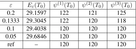
solution (and their gradients) for runiand the computed reference solution (with ∆t = 0.001, N = 1000). The definition of the norms are given in (4.3) and EOC in (4.1). We provide estimated orders of convergence between subsequence steps. . . 108 4.3 The table displays the results of the first test series. The value of the

sur-factant potentialqεis taken at the point 0,

√ 3 2

at different sizes of. ‘ref ’ is the solution of the sharp interface problem(4.5)at the points=L. The notation is defined in(4.1)-(4.2). . . 113 4.4 The table displays the results of the second test series. The value of the

surfactant potentialqε is taken at the point 0,

√ 3 2

at different sizes of. ‘ref ’ is the solution of the sharp interface problem(4.5)at the points=L. The notation is defined in(4.1)-(4.2). . . 113 4.5 The table displays the measured angles (discussed for the diffuse setting in

the test setup) of the test series at timeT0 = 0.4in the absence of

(7)

(8)

List of Figures

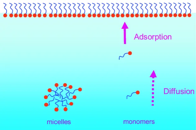
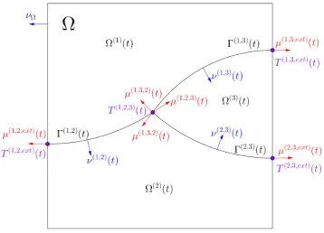
1.1 Schematic displaying surfactant molecular structure, and behaviour in so-lution including the adsorption monolayer formation. The image source is given in the Declaration. . . 2 2.1 We display geometric features of a domainΩpartitioned into three time

de-pendent subdomains Ω(i)(t), separated by interfacesΓ(i,j)(t) which meet at a triple junctionT(i,j,k)(t)and at the boundariesT(i,j,ext)(t). For com-pleteness we display the normals and conormals to the interfaces . . . 14 4.1 Inital conditions for a lens represented by solid lines. Ω(3) is trapped

be-tween two fluidsΩ(2)andΩ(3). The dashed and dotted lines represent snap-shots of the of the relaxation we expect at some timet1 > 0andt2 > t1

respectively in the absence of external forces. . . 102 4.2 Figure displaying the state of the system at timet =T0. The bottom right

displaysϕ(3)ε field, with ϕ(εi) = 0.5 level sets in white (appearing in all

diagrams). The top right shows pressure field. The left shows the velocity vector field where the size and colour of the arrows represent the magnitude of the velocity field. . . 105 4.3 Figure displaying the state of the system at timet=T0+ 0.5. The bottom

right displaysϕ(3)ε field, withϕ(εi)= 0.5level sets in white (appearing in all

diagrams). The top right shows pressure field. The left shows the velocity vector field where the size and colour of the arrows represent the magnitude of the velocity field. . . 106 4.4 Figure displaying the state of the system at timet = T0+ 1. The bottom

right displaysϕ(3)ε field, withϕ(εi)= 0.5level sets in white (appearing in all

(9)

4.5 The figure displays the total discrete energy valueE_εn, that is, the discreti-sation of (2.170)(see Section 3.2.3 for two phase matched density case). For clarity we have not displayed every solution in the test series, but have captured the full range of accuracies, and the reference solution is given by the solid black line. . . 109 4.6 A magnified section of Figure 4.5 displaying the right hand edge where the

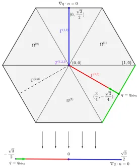
EOCs in Tables 4.1 and 4.2 were calculated. In this figure, the symbols are placed at every evaluation of the time stepping scheme . . . 109 4.7 Setup for theε-convergence test for the surfactant equation as considered

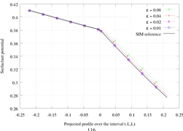
in Section 4.3.1. . . 110 4.8 The profile of the computed potentialqε at at differentεvalues and

com-pared to the solution of the sharp interface problem(4.5). Values were taken at timet= 0.01, and the diffuse approximation was sampled along the path displayed in Figure 4.7 and transformed to be displayed over the interval

−L, L

. . . 115 4.9 A magnified section of Figure 4.8 displaying the right hand end of the profile

of computed potentials. We display the solutions over the interval(L₂, L). . 115 4.10 The profile of theqε at different εvalues and compared to the solution of

the sharp interface problem (4.5). Values were taken at time t = 0.01, the diffuse approximation was sampled along a path as in Figure 4.7 and projected onto the interval −

√ 3 2 ,

√ 3 2

. The triple junction is centred at0. 116 4.11 A section of Figure 4.10 displaying the profile of the computed potentialqε

at at differentεvalues and compared to the solution of the sharp interface problem(4.5). We display the path only from −

√ 3 8 ,

√ 3 8

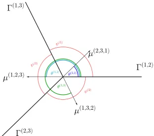
to observe the approximation of the triple junction. . . 116 4.12 Diagram of a triple junction between three hypersurfacesΓ(i,j) _{and their}

conormalsµ(i,j,k). The anglesθ(i,j)represent the angles described by the Neumann triangle relation of the surface tensionsσi,j, and the anglesψ(k)

are the angles between the corresponding branchesΓ(j,k),Γ(k,i). . . 117 4.13 Figure displaying the state of the system at timet=T0. We see theϕ

(·) ε =

0.5level sets for each phase field, as well as theϕ(1)ε =ϕ(2)ε =ϕ(3)ε = 1₃

level set points. We have coloured themε = 0.05(blue),ε= 0.1(green),

ε= 0.15(red) andε= 0.2(purple). . . 121 4.14 Figure displaying the state of the system at timet=T. We see theϕ(ε·) =

(10)

4.15 Figure displaying the state of the system at timet=T0. We see theϕ( ·) ε =

ε= 0.15(red) andε= 0.2(purple). . . 123 4.16 Figure displaying the state of the system at timet=T. We see theϕ(ε·) =

level set points.We have coloured themε = 0.05(blue), ε = 0.1(green),

ε= 0.15(red) andε= 0.2(purple). . . 123 4.17 Figure displaying the state of the system at timet = T0 for ε = 0.1test

run. The left displays theϕ(ε·) = 0.5level sets for each phase field over the

background showing surfactant potential (hereq = 0). The right displays the velocity stream lines coloured by their magnitude. . . 127 4.18 Figure displaying the state of the system at time t = T0 + 0.6. The left

displays theϕ(ε·) = 0.5level sets for each phase field, the black lines show

a reference solution without surfactant. The white shows the effect of the background surfactant potential displayed. The right displays the velocity stream lines coloured by their magnitude. . . 128 4.19 Figure displaying the state of the system at timet=T. The left displays the

ϕ(ε·) = 0.5level sets for each phase field, the black lines show a reference

solution without surfactant. The white shows the effect of the background surfactant potential displayed. The right displays the velocity stream lines coloured by their magnitude. . . 128 4.20 Figure displaying the state of the test series at timet = T. We see the

ϕ(ε·) = 0.5 level sets for each phase field, as well as theϕ(1)ε = ϕ(2)ε = ϕ(3)ε = 1₃ level set points. From Left to Right, we have theε= 0.05(blue), ε= 0.1(green),ε= 0.15(red) andε= 0.2(purple). . . 129 4.21 Figure displaying thex-coordinates of the right hand triple junction of each

lens over the periodt = 0tot = T charted in ParaView. The final step is shown by Figure 4.20. The time step number of the printed solution is

τ = 10∆t= 0.1and so the surfactant is introduced atT0 = 24τ and final

time is T = 65τ. The displayed profiles are for ε = 0.05 (blue cross),

ε= 0.1(green square),ε= 0.15(red plus) andε= 0.2(purple circle). . . 129 4.22 Figure displaying the L2 norm of the velocity over the period t = 0 to

t=T. The surfactant is introduced att= 2.4, and the final step is shown by Figure 4.20. The displayed profiles are forε= 0.05(blue cross),ε= 0.1

(11)

4.23 Inital conditions for a coupled bubble represented by solid lines. Ω(1) is an encapsulating fluid containing a coupled droplet of two fluidsΩ(2)and

Ω(3)_{. The left demonstrates the}_ϕ(1)

ε = 0.5level set resolution. The middle

displays a slice aty = 0ofϕ(1)ε and the right displays the same slice with

initial values forϕ(2)ε . . . 131

4.24 Dynamics soon after initial conditions att = 0.1. The left hand side dis-plays theϕ(1)ε = 0.5 level set coloured by theϕ(3)ε phase (shows the

dif-ferentiation between the coupled droplets). The right hand side displays the pressure over a slice with velocity field given by the glyphs - large red arrows are higher velocity. . . 134 4.25 Dynamics soon after initial conditions att = 1.4. The left hand side

dis-plays theϕ(1)ε = 0.5 level set coloured by theϕ(3)ε phase (shows the

dif-ferentiation between the coupled droplets). The right hand side displays the pressure over a slice with velocity field given by the glyphs - large red arrows are higher velocity. . . 135 4.26 Snapshot taken soon after initial conditions att = 0.04. The level sets of

the surfactant concentration are shown, the inflow concentration is around

0.28at the top of the domain, as the snapshot is taken during the relaxation period(T0, T0+Tq). . . 135

4.27 Dynamics soon after initial conditions att= 0.04. Displayed is theϕ(1)ε =

0.5level set coloured by theϕ(3)ε phase (shows the differentiation between

the droplets). The left hand side displays the simulation with surfactant present, the right hand side displays the simulation with no surfactant present.136 4.28 Dynamics soon after initial conditions att= 0.2. Displayed is theϕ(1)ε =

the droplets). The left hand side displays the simulation with surfactant present, the right hand side displays the simulation with no surfactant present.136 4.29 Dynamics soon after initial conditions att= 0.33. Displayed is theϕ(1)ε =

(12)

Acknowledgments

I am indebted to both of my supervisors Bj¨orn Stinner and Andreas Dedner for their

guid-ance, honesty, and at times their considerable patience. I would also like to thank my

examiners James Sprittles and Vanessa Styles, who had the perseverance to read, correct

and examine me on this thesis, and to Dwight Barkley for advising on the examination and

for chairing my personal advisory committee in the last 3 years. Also to all others with

whom I have consulted, and worked with, or those who have helped proofread my thesis, I

thank you.

I also would like to thank my parents Chris and Alistair and my sister Charlotte, I

am overwhelmed by their persistent love and support. As well as their frequent supplies of

vegetables, honey, eggs, and generally hilarious company.

I would like to thank all my friends of MASDOC and at Warwick who have made

life as a PhD student into a true pleasure. Those in my cohort deserve a special credit,

in order of proximity to my desk, thank you to John, Jack, Jamie, Adam, Yulong, Luke,

Rodolfo, and Matt. Also to the lost MASDOC’er Jake who has remained a great friend.

To Rebecca, the girl who has kept me sane by pretending to listen for hours on end

about the hardships of a PhD life, who has given me so much love and support in these last

few months, which have kept me on track and happy through all the stress. I love you, and

thank you.

I would like to thank the MASDOC centre and all of its staff and the training it

provided, and to the Mathematics department for their wine and Statistics department for

their coffee. Finally, I would like to thank EPSRC and as this work was supported by their

(13)

Declarations

This thesis is submitted to the University of Warwick in support of my application for the

degree of Doctor of Philosophy. It has been composed by myself and has not been submitted

in any previous application for any degree.

The work has been carried out by myself. There has been collaboration in Chapter

2 with Bj¨orn Stinner, and I was given support for the code development from Andreas

Dedner. The use of code packages and numerical libraries from other developers has been

well documented in Chapter 1.

Figure 1.1 in the introduction was originally from

(14)

Abstract

We investigate a free boundary problem arising in fluid dynamics, by modelling

multiple incompressible fluids over subdomains with different material quantities, and in the

presence of surface tension reducing chemicals known as surfactants. We construct a free

energy for this system, and we require it obey the second law of thermodynamics, leading

to the formulation of an energy minimisation problem (the sharp problem). This problem

is degenerate, so we regularise it by constructing a new energy of Ginzburg-Landau type,

parametrised by a (small) constant >0and when→0the sharp problem is recovered in

the sense ofΓ−convergence. This multi-phase energy is formed from a multiwell potential

and gradient term, and the minimisers are known as phase field variables. The phase field

variables approximate characteristic functions of the subdomains, and the model is rewritten

as functions of them. Beneficially, the energy analysis can be repeated as before to obtain a

diffuse interface model.

We construct and perform numerical analysis of a novel discretisation scheme for

a Cahn-Hilliard Navier-Stokes system. Here we create a fractional-theta coupling scheme

which is importantly proved to be of second order in time. The key property of this scheme

is that it uses weighted operator splitting to separate the different nonlinearities that appear

in a Cahn-Hilliard Navier-Stokes system. That is, the Cahn-Hilliard multiwell potential, the

incompressibility condition and the convection. We discuss stability and the extension to

surfactants. We implement the novel scheme in DUNE (Distributed Unified Numerics

En-vironment), a finite element package and use simulation to run tests to validate the stability

and consistency of the schemes, convergence of the diffuse interface model with respect to

(15)

Chapter 1 Introduction

1.1 General introduction

Surfactants (surface active agents) are chemicals which are identified by their ability to lower the surface tension along the interfaces between different fluids. The reduction of

surface forces is caused by the chemical structure of the molecules: they are amphiphilic,

that is, they have a hydrophilic (water attractive) head and hydrophobic (water repulsive) tail. It is therefore beneficial for the surfactant to adsorb to fluid-fluid interfaces, that is,

to form an oriented, single molecule thick layer there. Figure 1.1 displays this process and

furthermore shows the tendency of surfactants to self assemble into complex bulk structures such as micelles. At high concentrations they may also self assemble to form bilayers [86],

vesicles, and even liquid crystal lattices [132], these structures minimize contact between

the repulsive tails and the surrounding solution. The behaviour and formation of the single layers along fluid interfaces can vary widely due to solubility of the surfactant in the fluids,

and the interactions between the molecules such as electrostatic forces of polar surfactants. Having formed these monolayers, the surfactant cannot bond as strongly to other molecules

as the pre-existing liquid-liquid bonds can. It requires less energy to break these bonds,

and the surface tension is reduced. The chemistry of these products are widely known, for example, these are explained in the introductory chapters of [78, 99].

The importance of manipulation of surface tension can be seen in the change of

force balance within the fluid. Consider a regime where surface forces dominate a fluid’s evolution. If a surfactant is then added, inertial or viscous forces may dominate over the

now reduced surface tension (possibly by several orders of magnitude, see [110]) leading to

different drivers of evolution and hence an altered macroscopic behaviour. A good review of Marangoni forces, the induced dynamics due to concentration gradients across liquid

(16)

[image:16.595.163.479.104.314.2]

Figure 1.1:Schematic displaying surfactant molecular structure, and behaviour in solution including the adsorption monolayer formation. The image source is given in the Declara-tion.

[123], and some examples of the surfactants that induce these behaviours in [111].

Surfactants can occur naturally and are vital to a wide range of physical,

chemi-cal and biologichemi-cal systems [125]. Material scientists may also synthesize surfactants from natural (fatty acids and alcohols) or petrochemical ingredients. The ability to control the

chemical structure and concentrations of the surfactants in a solvent, has lead to a wealth

of commercial products, such as detergents, dispersents, wetting agents, emulsifiers (for example in oil recovery [115]), and in industries such as agrochemicals, pharmaceuticals

and cosmetics. A more complete view of the vast scale of applications for different species

of surfactant is given in [125].

This thesis focuses on activity of surfactants in a system of more than two fluids.

In many of the industries mentioned, there are applications involving these systems. For

example there is great interest in surfactant effects to water-in-oil-in-water emulsions, in the food industry for naturally occuring emulsions [83], or in pharmaceutical or cosmetic

industries for prolonging drug release [87, 74]. Surfactants used in enhanced oil recovery are introduced to stabilize foaming for ternary solutions [107] or non aqueous solutions

[51].

Many surfactant induced phenomena have been examined experimentally in mate-rial science. More recently in applied mathematics, the simulation of these systems has

be-come possible through developments of mathematical tools and computational techniques

(17)

model a system of fluids, each described by the incompressible Navier-Stokes equations in

isothermal conditions, and demarcated by material parameters such as mass densityρand dynamic viscosityη([63]).

In order for Newton’s laws to hold, these equations are supplemented with derived

interfacial force conditions where two fluids meet, and some contact line force conditions if

three of these dividing interfaces meet at a triple junction. From this mathematical perspec-tive, the aforementioned effects of surfactants on their environment are modelled, through

the form of force balancing conditions and their dependence upon the concentration of

ad-sorbed surfactant at the fluid-fluid interfaces.

1.2 Thesis contributions

The objective of this thesis is to provide new developments towards modelling surfactants in multi-phase flow in two core areas.

First, we construct a diffuse interface model extending [54] (which investigated

two phase flow with surfactant) to three or more phases. We emphasize the inclusion of surfactants dissolved in three fluids and adsorbed along interfaces between them. In some

applications surfactant mixtures are used [109], for simplicity we shall only model a single species of surfactant, however it is a straightforward generalization to multiple surfactants

and is remarked upon when relevant. We also present numerical simulations to support

some analytic results.

Second, we propose a new numerical timestepping scheme for multi-phase flow

with surfactant based on the idea of a fractional time splitting introduced in [26]. The

nu-merical investigation tackles stability and consistency. Supported by nunu-merical benchmark-ing against several test problems, it demonstrates the scope and accuracy of the scheme. We

also assess the validity of the model we construct in this way, by looking at both qualitative

and quantitative simulation for benchmarks of multi-phase fluid with surfactant.

The fundamental mathematical technique we apply is known as phase field

mod-elling [8]. This is a method for approximating a system with several interacting (usually

time dependent) subdomains that cover a domain of interest by replacing the separating hypersurfaces between domains with thin interfacial layers of a (small) positive interface

width, denoted byεthroughout. These are described by a phase field variable (or order pa-rameter) which distinguishes between different phases. In the bulk phases, the phase field variable takes a near-constant value, and in the interfacial layers, it smoothly changes value

between the different constants. A good introduction to these “diffuse” methods for fluid

(18)

1.2.1 Diffuse interface model of surfactants in multi-phase flow

Many methods exist for accounting for different classes of surfactants. For insoluble

surfac-tants, which are modelled with no bulk presence, one can describe their evolution and be-haviour purely from their interfacial concentrations. Here, research directions are directed

to methods which accurately and efficiently predict the interface evolution. In particular

techniques that exploit the fact that the interface dimension is one less than the bulk, and treat the surfactant efficiently with a surface partial differential equation. One popular idea

is that the interface can be tracked explicitly with marker particles (Lagrangian points [45]),

that is, the computational mesh tracks the interface. These may be coupled with a Navier-Stokes solver, such as an embedded boundary method [84]. One may also use tracking

for the interface but solve for the surfactant using a finite volume method [68, 88]. Another

field of investigation is for solving problems over a fixed grid and employ techniques to cap-ture or reconstruct the interface, such as volume of fluid methods [73] (relying on volume

conservation to construct the interface), level set methods [138] (a level set of a function

represents the interface [101, 102]) or novel fixed grid methods such as segment projection methods [79] (the interface is segmented and parametrised by simple functions on chosen

coordinate planes). Finally, one may use a carefully chosen smoothing function that pre-serves key mathematical structure, and replaces the (sharp) hypersurface with a (diffuse)

thin interfacial region. This technique is known as a phase field model or diffuse interface

model [92], with a more general discussion in [8]. One particular benefit of this method over any others mentioned (including the level set formulation), is that the approximation

it provides to the free boundary problem is more mathematically grounded. In particular

there is much stronger notion of convergence as our interfacial region shrinks to a hypersur-face, and this allows for the recovery of the equations for the entire free boundary problem.

We shall utilize this latter method in this thesis, and the corresponding asymptotic analysis

which characterises the recovery will be presented in a forthcoming article [42].

Methods have also been developed for soluble surfactants, that is, where the

sur-factant is present as both an interfacial quantity as a monolayer concentration, and a bulk

quantity dissolved in one or more of the fluids. The difficulty of this extension is twofold: we must both solve for the bulk surfactants and the behaviours they may exhibit (such as

structure formation [132]), and we must account for kinetics of the surfactant

adsorption-desorption process (the formation of a monolayer along a fluid-fluid boundary). In different scenarios, either factor may dominate in influencing the system dynamics. Typically the

surfactant is modelled by a surface PDE at the interfaces and also a bulk PDE within each

fluid region where it is soluble. These are coupled by boundary conditions related to the ki-netics of the adsorption-desorption process. In early attempts, the surfactant was accounted

(19)

diffusion and assumption that the concentration of surfactant was near constant in the bulk

[75]. Developments have lead to solving in the bulk regions too. This can be handled with

explicit tracking [32, 98], redistributing mesh methods [14] or embedded boundary methods [80] as in the insoluble surfactant case, assuming an equilibrium relation for the sorption.

The fixed grid reconstructions and interface capturing methods have also been developed

in this direction - see, for example level set methods [139] and the phase field methods [46, 127, 92].

Despite the high accuracy of the explicit tracking methods, fixed grid capturing

methods are widely studied as well, as they allow for more complex dynamic geometrical features to be accounted for naturally. In particular, they may describe fluid systems which

undergo topological changes. This is because the information pertaining to the geometry

of the problem is contained within fields and equations and not within the mesh grids or computational set up. Problems of geometry then become problems in partial differential

equation theory, and so the library of techniques for differential equations can be utilized to solve them.

We discuss phase field methods in this thesis, and in this case the aforementioned

fields known as phase field variables are subjected to the Allen-Cahn or Cahn-Hilliard equations (orginally in [30, 29]). The reformulation not only approximates the geometry

of the original problem but also the accompanying energy framework. In fact, it has been

known [96] that the system energy for the phase field model (ordiffuse interface model) will converge (in the sense ofΓ-Convergence [24]) to the system energy of the model it

approximates (the sharp interface model) as the width of the interfacial region tends to 0. In particular, this means that the minimisers of the diffuse interface model energy will converge strongly to minimisers of the sharp interface model energy. This fact potentially

provides significant benefit over other interface capturing approaches, as it increases the

amount of information that is recoverable through the interface representation, for example, by preforming an asymptotic analysis. For application of this technique to a Stefan problem

see [49], and for examples of recovered equations from curvature driven evolution see [52].

The governing equations of the previous techniques required an equilibrium rela-tion known as an isotherm (for example [85], which connected the surface and bulk fields.

Analysis [136, 39, 40] and experiments [76] have shown that this assumption implies that

the rate of any kinetic properties (for example orientation of molecules or effects of inter-molecular charge forces) can be quick relative to the timescale of diffusion when forming

the surfactant monolayer at interfaces. This is a good approximation for certain non-ionic

surfactants out of mixture, however for ionic surfactants, or larger molecule surfactants, this equilibrium is not immediately satisfied. The relevant extension to the free energy

(20)

analysis in [54], where a thermodynamically consistent model for soluble surfactant in two

phase flow is considered.

Extending work in [54], we generalize the model of a binary flow found in [1] to the multi-phase (i.e three or more phases) case and include the presence of a soluble

surfactant. In particular we use a vector phase field (diffuse interface) model construction

and focus our study on the modelling of contact lines or triple junctions where three fluid-fluid interfaces meet. The model for theM ≥3phases we consider is that of a vector Cahn-Hilliard type system, which is a partial differential equation over the domain, for order

paramaters (phase field variables)ϕε = (ϕ(1)ε , . . . , ϕ(εM)), parametrized by an interfacial

layer widthε. Their motion is governed by two features of the energy framework. The first is a smooth multi-well potential that ensures the lowest energy states will take the form

whereϕεapproximatesek(thekthstandard basis vector) in the fluid region (or “phase”)k.

The second energetic feature is a multi-phase gradient energy that ensures the phase field

variables are regularized enough so that they smoothly transition between valueseiandej

across interfacial layers or contact regions between 3 phases.

We describe fluid flow through the language of continuum mechanics, that is, from

a macroscopic scale - treating molecular effects as negligible. Studying from this viewpoint involves finding the velocityv(x, t), the pressurep(x, t)at any point in the fluid volume

x∈ Ω ⊂ _Rd_,_d_{= 2}_,₃_{and time interval}_t _∈ _[0_{, T}_]_{. The individual flows (i.e phases) are}

assumed incompressible, and so the fluid densityρ(x, t)is assumed constant within the bulk region of each fluid. The phase fieldsϕεdescribe the geometry, thus the density variation

originates from the dependenceρ≡ρ(ϕε), acting as an interpolation over interfacial layers between bulk density values. Other material quantities that are constant in each fluid phase, such as viscosity, are attributed a similar dependencyη≡η(ϕε).

The limiting model whenε→0, known as the sharp interface model, also involves a natural free energy framework. It is a classical description of the system where one as-sumes that the interfaces between fluids can be represented as hypersurfaces and is the basis

of front tracking approximation methods. It is derived using the same procedure as for the

phase field model: We postulate balance equations for the fluids. These are supplemented with corresponding interface force balance equations between phasesiandj by opposing surface tension forcesσi,j (as in [103]) with bulk fluid pressures and viscous stresses. We then use the system energy to derive constitutive assumptions and suitable boundary con-ditions to close the system and ensure thermodynamic consistency. This consistency is the

agreement of the model with the second law of thermodynamics, that is, the decay of the

global system energy over time.

The surfactants are accounted for through the surface tension σi,j ≡ σi,j(c(i,j))

(21)

arises as the surfactants are themselves subject to fluid transport, and will depend on the

ge-ometry of the interfaces. To derive the corresponding approximating phase field model for

the surfactants, we are motivated by the work of [6] and [54] which we extend to multiple phases. The equivalence between distributional forms for interfaces and contact lines, with

using characteristic test functions of these features allows us to reform our surfactant

con-centration equations in the latter form. We regularize the characteristic functions, using the carefully chosen distributions, and then construct surfactant dependent free energies which

also satisfy energy decay laws under corresponding conditions. This flexible approach

al-lows for solubility of the surfactant in one or more phases, and receives benefits of the phase field formulation described earlier.

In Chapter 2 we first present our sharp interface description of the problem in

Sec-tion 2.1. We use mass and momentum balance equaSec-tions to derive the governing equaSec-tions, and close the system with appropriate boundary conditions and constitutive assumptions

that lead to a thermodynamically consistent system seen in Section 2.1.8. In Section 2.1.9 we consider the particular case of local equilibrium of the surfactant potential around

inter-faces and present the resulting model in this case in Section 2.1.10. Finally we state some

choices for the adsorption isotherms under this equilibrium. In Section 2.2 we present the diffuse interface description of the problem. We follow similar methods as in the sharp

in-terface case and arrive once more at a thermodynamically consistent system seen in Section

2.2.5. We then proceed with the diffuse approximation of the case of local equilibrium of the surfactant potential and present this model in Section 2.2.7. We finally list some

pos-sible choices for mobilities and multiwell potentials for the phase field model in Section

2.2.8.

1.2.2 A scheme for multi-phase flow

The notion that a fluid interface could have a nonzero thickness, and this thickness could be determined by an equation of state due to a density profile, dates back to the work of

Rayleigh and van der Waals [112, 113]. The theory was built upon by Korteweg [82],

to construct constitutive laws for the fluid stress tensor in terms of density and density gradients. The ideas were then reformulated by Cahn and Hilliard [30, 29], with regards

to a more general construct of a phase field variable. One of the earliest approaches for

modelling binary fluids through this phase field approach was the so called “model H” introduced by [71] which used a Cahn-Hilliard equation with a (soft enforcing) smooth

phase field potential for the phase field coupled to the Navier-Stokes equations with constant

mass density for the fluid mechanics. This construction was formulated with a restriction on the mass density of the fluids, and more recently was shown to obey a form of the second law

(22)

lead to the extension of this original model to include varying mass densities [93], and more

recently to enforce divergence free velocities ([41, 20]) and also frame indifference and

thermodynamic consistency [1]. These properties greatly improve the quality of numerical schemes which can be constructed for these models.

Many schemes in the literature currently available for multi-phase flow, are based

on robust schemes for the phase field systems, to which the fluids scheme is then attached. In practice, the fluid mechanics becomes very expensive to solve accurately especially with

large Reynold’s numbers [134] or large density variations between different phases. We

take a different approach. We inspect the literature ([89]) for a reliable scheme for general incompressible fluids, and this we then develop into an accurate and efficient scheme for

multi-phase flow, which is shown to be stable in several diverse test problems. We now

describe the current state of the field for these types of fluid systems.

A large class of methods for incompressible flows are corrective schemes (velocity

or pressure), created by Chorin [33, 34] and Temam [128, 129]. In pressure correction, the most basic scheme comprise two substeps. In the first step, one solves for a velocity field

while treating the pressure with some degree of extrapolation (perhaps using a previous

timestep as the approximation). In the second step, one projects the computed velocity into a desired solution space - a divergence free Sobolev space.

Numerical boundary layers limit this accuracy to first order, unless one takes more

complex forms of the scheme ([64]) and use more previous timesteps for extrapolation. The benefits of these schemes are to separate the treatment of the two core difficulties of the

incompressible Navier-Stokes: the incompressibility constraint and the inertial effects.

Ve-locity correction methods are similar (in fact, regarding error analysis, they are equivalent), but the substep order is reversed compared with the pressure correction. Evidence suggests

they are more stable than pressure correction for second order or higher accuracy [116, 77],

though typically less easy to implement. They still contain boundary layers which limits accuracy. Consistent [65], and Gauge-Uzawa [100] methods eliminate artificial splitting

errors and results are compared in [64].

There have been generalizations of these splitting techniques for variable density flows for finite differences by [16, 5], and, additionally, for finite volumes and finite

ele-ments [50, 66]. A novel form of the Navier-Stokes equations is presented in [66], which

conserves kinetic energy in the discrete setting. This property has lead to the development of an unconditionally stable scheme for three phase Cahn-Hilliard-Navier-Stokes in [95].

The difficulty addressed in this thesis is to create a coupling scheme which allows for the

Cahn-Hilliard system to be transported by a non divergence free velocity field, and for this scheme to ensure decay of the discrete system energy over time. More recently

(23)

have obtained some results for convergence and stability even for higher density ratios. A

two phase flow scheme has been constructed using these techniques by Shen and Yang in

[117, 118, 119].

We wish to investigate another promising class of splitting methods, which solve

time discrete initial value problems by splitting the physical time interval into subintervals

and solving different problems over different subintervals. These can be thought of similar to Strang splitting [124], and a good introduction can be found in [60]. The key assumption

of these schemes are that the system operatorF can be decomposed into F = F1 +F2,

whereF1andF2are mathematically simpler objects thanF. In the incompressible

Navier-Stokes, these will be an operator for the incompressibility (a Stokes type operator) and a

convection type operator for the inertial term (a Burgers type operator). The simplest case

of these splittings, is the Peaceman-Rachford scheme [104], where one splits thenth time interval[n∆t,(n+ 1)∆t]of size∆tinto two equally sized subintervals about the midpoint

(n+ 1₂)∆t. The Peaceman-Rachford scheme [104] solves for a solution with F1 taken

implicitly and F2 taken explicitly in the first half-step, then F2 taken implicitly and F1

taken explicitly in the second step. One can demonstrate from eigenvalue analysis that this

scheme is very accurate, of second (almost third) order accuracy [60] in time, however there are issues with slow convergence similarly observed in a Crank-Nicholson scheme (which

is in fact a particular case of the Peaceman-Rachford scheme), making it an inappropriate

choice for stiff systems.

A promising scheme from this field (with praise in [134]) is the fractional theta scheme. This scheme contains three substeps,[n∆t,(n+θ)∆t], [(n+θ)∆t,(n+1−θ)∆t]

and[(n+ 1 −θ)∆t,(n+ 1)∆t]. Solving for the variable u, the split system operator

F(u) =F1(u) +F2(u)forms the fractional scheme as follows:

1. [n∆t,(n+θ)∆t], lengthθ∆t, solve the substeptn→tn+θ,

un+θ₋_un

θ∆t +F1(u

n+θ_{) +}_F

2(un) = 0 (1.1)

2. [(n+θ)∆t,(n+ 1−θ)∆t], length(1−2θ)∆t, solve the substeptn+θ→tn+1−θ,

un+1−θ−un+θ

(1−2θ)∆t +F2(u

n+1−θ_{) +}_F

1(un+θ) = 0 (1.2)

3. [(n+ 1−θ)∆t,(n+ 1)∆t], lengthθ∆t, solve the substeptn+1−θ →tn+1,

un+1₋_un+1−θ

θ∆t +F1(u

n+1_{) +}_F

(24)

So the operator F1 is treated implicitly-explicitly-implicitly over the timestep, andF2 is

treated explicitly-implicitly-explicitly. With correct choice ofθone can obtain second order accuracy, strong A-stability, and thus demonstrate robustness regarding stiff systems. This method has been applied to the Navier-Stokes equations by [26] and a finite element method

for the spatial discretisation has been analyzed by [81] and [97] for fixed densities. The

stability and accuracy of the scheme have been demonstrated in numerical simulations, such as [134]. Some of the good properties of the scheme can be shown through a link with

the Augmented Lagrangian formulation for saddle point problems [61].

We present a variable density form of the scheme, and show it still satisfies second order accuracy with the correct choice of theta. We further couple it to a Cahn-Hilliard

system by using a technique found in [36]. For this coupled system we perform a stability

analysis in the case of matched densities. In the variable density case we show consistency and verify this complication does not yield loss of accuracy.

In Chapter 3 we present the abstract fractional-theta scheme and then develop the operator splitting for the fixed density two phase Cahn-Hilliard Navier-Stokes scheme for

the weak time discrete problem in Section 3.1.2. We present the fully discrete scheme in

Section 3.2.1, and investigate stability for the discrete energy in Section 3.2.3. Extensions to multiple phases and variable density are formed in Section 3.3 and Section 3.4. The proof

that the variable density scheme is of second order accuracy in time is in Section 3.4.2.

1.2.3 Benchmark testing

We additionally provide validation to our modelling framework and our numerical schemes

by using simulation benchmarks for qualitative and quantitative verification in Chapter 4. We assess the scheme by validating the second order accuracy in time proved in

Chapter 3 and to commenting on stability in Section 4.2. We construct a relaxing liquid

lens problem for three fluids of variable density and comparison of discrete solutions to a reference solution on a very fine time step resolution gives us orders of convergence, which

we find to be of second order for the velocity.

To assess the validity of the diffuse interface model constructed in Chapter 2, we investigate the convergence of the surfactant equations as the interfacial width parameterε

tends to 0. We demonstrate this in Section 4.3.1 by setting up a test problem in which a

flow of surfactant travelling through a stable, relaxed, triple junction. We compare this to the solution of the corresponding sharp interface solution and observe the convergence. We

also present a qualitative simulation for the convergence asεis reduced of the marangoni effect on a triple junction, for a liquid lens in Section 4.3.3. We find that if the interfacial width is large then interfacial effects are more dominant over inertial effects in the bulk,

(25)

with soluble surfactant is still novel for phase field descriptions, this provides insight into

the size ofε which may be required in for accurate results. We finally demonstrate the flexibility of the scheme by considering a rising coupled droplet in three space dimensions with surfactant in Section 4.4. Here we use a qualitative example to demonstrate the effects

of surfactant presence on a variable density multi-phase flow. We run two experiments,

with and without surfactants and observe the changes in behaviour of the droplets that are captured by the simulation. In particular the surfactants induce a topological change as the

coupled droplet decouples into two disjoint droplets.

The reader is additionally directed to the YouTube channel, where I have records of some of the videos from simulations in the thesis.

https://www.youtube.com/channel/UC0K4vFNJzPyiHofVOU8aAJg

1.2.4 Software development

The software element to this thesis required substantial effort, and thus, the tools used

throughout were of vital importance. This section highlights the key software that was

developed and used of for the duration of the project. Documentation and cleanup of this code will shortly be completed, for other users.

The implementation for the numerical schemes were performed using the

Dune-Fem toolbox, part of DUNE(-2.5) Distributed and Unified Numerics Environment. DUNE is a modular software for solving partial differential equations using methods such as finite

elements, finite volumes and finite differences, of which we use the first extensively in our

code. We direct the reader towww.dune-project.org/modules/dune-fem/for

the current software webpage, and cite [38] for an overview of the core principals of this

module and accompanying Dune-Fem-Howto module with accompanying documentation

for some example code. The Navier-Stokes solver is already in use by other members of DUNE development team. The version control and writing of software was managed by

creating a git repository on GitLab and creating a new module where the software and some supporting documents are kept.

We utilize some external software in the finite element simulations. For grid

man-agement we use ALUGrid, through the module Dune-ALUGrid [4], which provides the parallelizable adaptive grids that are used in the grid construction. Also linked in are some

external solvers (direct and iterative) for linear systems and corresponding preconditioners.

These use the flexible PETSc interface [12, 11, 13], where we make use of the UMFPACK SuiteSparse package [37] for serial problems, the MUMPS direct matrix solver [7], and the

HYPRE BoomerAMG preconditioner [47] for parallel problems .

(26)

so-lutions from the simulation, and for graphical output, I have used GNUPlot. I have written

some finite difference simulations (for example in the epsilon convergence tests) in

(27)

Chapter 2 Models

We begin by deriving a model for multi-phase flow with surfactant. It is an extension of

the work [54] which studied two phase flow with surfactant. Firstly, we fix the notation and terminology of the thesis. Then we derive a model using local balance laws of mass

and momentum, giving rise to a free energy formulation of the problem. By considering a

suitable free energy, we can pose constitutive assumptions and find closing conditions and natural boundary conditions for our problem. The summary of this sharp interface model

will be described in Section 2.1.8. We also note an important version of the model, when

it is under the assumption of local chemical equilibrium, which will ease the numerical simulation. This is summarised in Section 2.1.10.

We approximate the sharp interface model (2.58) – (2.67) with a phase field

method-ology. The construction of the phase field model follows similarly to the derivation of the sharp interface model, and these links will be noted throughout. The balance laws, free

energy formulation and choices of constitutive assumptions are detailed in subsequent

Sec-tions 2.1.2 to Section 2.1.5 and the summary of the diffuse model approximating (2.58) – (2.67) can be found in Section 2.2.5. Under a local chemical equilibrium at interfaces, the

model (2.82) – (2.90), also has a diffuse interface counterpart. This is detailed in Section

2.2.7.

The ending of this chapter deals with some more specific choices of key potentials

(28)

2.1 Sharp interface model

2.1.1 Notation and preliminaries

LetΩ⊂_Rd_,_d_{∈ {}₂_,₃_}_{, be a bounded domain and}_I _{= (0}_{, T}₎_,_T _∈_[0_,_∞₎_{be a time}

inter-val. Assume thatΩis partitioned by moving hypersurfacesΓ(i,j)(t)intoMtime dependent open subdomainsΩ(k)₍_t₎_,_{i, j, k} _{∈ {}₁_{, . . . , M}_}_{. Intersections of three hypersurfaces are}

denoted byT(i,j,k)(t)and form triple points (d= 2) or form triple lines (d= 3) ending in quadruple pointsQ(i,j,k,l)(t),i, j, k, l∈ {1, . . . , M}. For simplicity, with regards toT(i,j,k)

we will only talk abouttriple junctionsin the following. Similarly, on the external boundary

∂Ωthere are triple points or linesT(i,j,ext)(t)with quadruple pointsQ(i,j,k,ext)(t)ifd= 3. The unit normal onΓ(i,j)(t)pointing out ofΩ(i)(t)intoΩ(j)(t)is denoted byν(i,j)(t)and byνΩ on ∂Ω. For the conormal ofΓ(i,j)(t) inT(i,j,k)(t) pointing intoΩ(k)(t)we write

µ(i,j,k)(t), and we writeµ(i,j,ext)(t)for it on∂Ω. Figure 2.1 is a sketch of a configuration as we have it in mind. Henceforth, for brevity, we omit writing the time dependence of

[image:28.595.139.498.365.623.2]

these objects.

Figure 2.1:We display geometric features of a domainΩpartitioned into three time depen-dent subdomainsΩ(i)(t), separated by interfacesΓ(i,j)(t) which meet at a triple junction

T(i,j,k)(t)and at the boundariesT(i,j,ext)(t). For completeness we display the normals and conormals to the interfaces

(29)

Ω→ _Rd_{, i.e., for each point}_x _∈ _Ω(i)₍_t₎_{there is a point}_x

0 ∈ Ω(i)(0)such thatx = ζ(t)

whereζ : [0, t] → Rdis the solution to∂˜tζ(˜t) = v(˜t, ζ(˜t))with initial valueζ(0) = x0,

and similarly for the interfaces, triple junctions, and quadruple points. We assume the fluids are immiscible, and so interfaces are impermeable. An implication of the properties ofvis that

[v]j_i = 0, u(i,j)=v·ν(i,j) onΓ(i,j), (2.1)

where [·]j_i = (·)(j) −(·)(i) stands for the jump from domain Ω(i) into Ω(j) across the

interface Γ(i,j) _and_u(i,j) _{is the normal velocity of} _Γ(i,j) _{in direction} _ν(i,j)_{. The match}

of tangential components of the velocity is typically required for stable viscous fluid-fluid

interfaces [15], although recently it has been shown that polymer fluids are modelled with

slip conditions [105]. Furthermore

u(i,j,k) =P₍_T(i,j,k)₎⊥v inT(i,j,k), (2.2)

whereu(i,j,k)is the normal velocity ofT(i,j,k)andP₍_T(i,j,k)₎⊥is the projection to the plane

normal toT(i,j,k).

Further notation concerns the material velocity for a fieldw: [0, T)×Ω→_R,

∂_t•(v)w:=∂tw+v· ∇w. (2.3)

Thanks to the above assumption that velocity transports the interfaces, this operator is

well-defined for fields restricted to a hypersurfaceΓ(i,j). We denote the surface derivative and

divergence along the hypersurfaceΓ(i,j)by∇_Γ(i,j) and∇_Γ(i,j)·, respectively. Some useful

identities such as a transport identity on evolving surfaces and integration by parts formula

on surfaces are provided in Chapter 6.

2.1.2 Balance equations

M ∈Nrepresents the number of fluids we consider in our system. They are assumed to be immiscible, incompressible, and Newtonian, and each fluid occupies a subdomainΩ(i)(t). Denoting byρ(i)the mass density of fluidi∈ {1, . . . , M}, the mass and linear momentum balances inΩ(i)read

∇ ·v= 0, (2.4)

∂t(ρ(i)v) +∇ ·(ρ(i)v⊗v) =∇ ·T(i), (2.5)

(30)

For simplicity we only consider a single surfactant. Its bulk and surface mass

den-sities are denoted byc(i)(t) : Ω(i)(t) → Rand c(i,j)(t) : Γ(i,j) → R, respectively. We consider only mass balance equations for surfactant and effects on the ambient fluids’ mass and momentum are neglected. This assumes that we model only a dilute surfactant solution,

and is taken implicitly in much of the literature, for example [19, 138, 137]. A range of

ap-plications for dilute surfactant can be explored in [125]. There are also apap-plications with high surfactant concentration where this modelling assumption is unsuitable, see [125, 83].

Following the derivation in [54] the surfactant mass balance equations read

∂_t•(v)c(i)=−∇ ·j_c(i), inΩ(i)(t), (2.6)

∂_t•(v)c(i,j)+c(i,j)∇_Γ(i,j) ·v=−∇_Γ(i,j)·j(_ci,j)+q_AD(i,j) inΓ(i,j)(t), (2.7)

wherej(c·)andj(

·,·)

c are associated bulk and surface diffusive fluxes andq(_ADi,j)is the

adsorp-tion desorpadsorp-tion flux. We determine the form of this sorpadsorp-tion flux and a closing condiadsorp-tion for the triple junction in the following calculation.

Let V(t) ⊂ Ω be an arbitrary material test volume, with V ∩∂Ω = ∅. Let

νV(x, t)be the external unit normal of ofV(t)andµ(Vi,j)(x, t)be the external conormal of V(t)∩Γ(i,j)(t)in∂V(t)∩Γ(i,j)(t). Letc(i), c(i,j)represent the concentration of surfactant dissolved into fluidsΩ(i)and interfacesΓ(i,j). This implicitly assumes the surfactants are soluble in fluid regions and may adsorb to all interfaces (discussion of this assumption is

found in Remark 2.1.1).

We integrate the balance equations (2.6) and (2.7) and sum over allΩ(·), Γ(·,·):

X

i

Z

V(t)∩Ω(i)₍_t₎

(∂_t•(v)c(i)+c(i)∇ ·v) +X

i<j

Z

V(t)∩Γ(i,j)₍_t₎

(∂_t•(v)c(i,j)+c(i,j)∇_Γ(i,j) ·v)

(2.8)

=X

i

Z

V(t)∩Ω(i)₍_t₎

−∇ ·j(_ci)+X

i<j

Z

(−∇_Γ(i,j) ·j(_ci,j)+q

(i,j)

AD ). (2.9)

We have used incompressibility of the fluid (2.4) here. Now we apply the Reynold’s

Trans-port Theorem (6.1) and the Surface TransTrans-port Theorem (6.2) to the integrals in (2.8):

d dt

X

i

Z

V(t)∩Ω(i)₍_t₎

c(i)+X

i<j

Z

c(i,j)

(31)

and we apply the Divergence Theorem to the integral ofj(ci)in (2.9) to obtain:

−X i

Z

∂V(t)∩∂Ω(i)₍_t₎

j(_ci)·νV −

X

i<j

Z

(j(_ci)·ν(i,j)+j(_cj)·ν(j,i)),

and finally we apply the Surface Divergence Theorem (6.4) to the integral ofj(ci,j)in (2.9)

to obtain:

X

i<j

Z

q_AD(i,j)−X i<j

Z

∂V(t)∩Γ(i,j)₍_t₎

j(_ci,j)·µ(_Vi,j)

− X i<j<k

Z

V(t)∩T(i,j,k)₍_t₎

(j(_ci,j)·µ(i,j,k)+j(_cj,k)·µ(j,k,i)+j_c(k,i)·µ(k,i,j)).

As the fluxj(ci,j)is tangential, the curvature term vanishes jc(i,j)·κ(i,j) = 0. Overall we

obtain:

d dt

X

i

Z

V(t)∩Ω(i)₍_t₎

c(i)+X

i<j

Z

c(i,j) (2.10)

= −X

i

Z

∂V(t)∩∂Ω(i)₍_t₎

j(_ci)·νV −

X

i<j

Z

∂V(t)∩Γ(i,j)₍_t₎

j(_ci,j)·µ(_Vi,j) (2.11)

+X

i<j

Z

(q(_ADi,j)−[j_c(·)]i_j ·ν(i,j)) (2.12)

− X i<j<k

Z

V(t)∩T(i,j,k)₍_t₎

(j(_ci,j)·µ(i,j,k)+j(_cj,k)·µ(j,k,i)+j_c(k,i)·µ(k,i,j)), (2.13)

due toV ∩∂Ω = ∅, we do not admit any boundary integrals. The identity reads that the (instantaneous) change of surfactant mass in the material volumeV(t) (2.10) is given by the surfactant mass flux across∂V(t)(2.11). In the absence of source or sinks, we wish for the mass of surfactant to be conserved over the test volume. Therefore we require that there

is no creation or destruction of surfactant during the adsorption-desorption process. With this in mind, we can determine a form of the sorption fluxes from (2.12):

q_AD(i,j)=j_c(i)·ν(i,j)+j_c(j)·ν(j,i)= [j_c(·)]i_j ·ν(i,j). (2.14)

We additionally define the more convenient one-sided sorption fluxq_ad(i,j)from domainΩ(i)

to interfaceΓ(i,j)through

(32)

soq(_ADi,j)=q_ad(i,j)+q(_adj,i). From (2.13), we assume the diffusive surface fluxes obey:

j(_ci,j)·µ(i,j,k)+j(_cj,k)·µ(j,k,i)+j(_ck,i)·µ(k,i,j)= 0 inT(i,j,k). (2.16)

We define a one-sided sorption fluxq(_adi,j,k)interfaceΓ(i,j)_to_T(i,j,k)_by,

q_ad(i,j,k):=j_c(i,j)·µ(i,j,k). (2.17)

The assumption (2.16) states that no surfactant mass is created, destroyed or stored in the

triple points ifd = 2nor in triple lines or quadruple points if d = 3. The triple junction contribution of (2.13) vanishes.

Remark 2.1.1. We have assumed for(2.10)–(2.13)that the surfactant is soluble in each fluid and adsorbs to all interfaces between fluids. However surfactants may be insoluble in some regionΩ(k) or may not adsorb to some interface Γ(k,l). This is often due to the compatibility of structures in the fluids and surfactants. Empirically it is measured by the hydrophile-lipophile balance (HLB) described in [78, 62] which assesses the strength of the hydrophilic subgroups of a surfactant against the lipophilic subgroup of the surfactant. For example, adding low HLB surfactants to an oil-water mixture causes water droplets to disperse in oil; a water-in-oil emulsion. Adding high HLB surfactants causes an oil-in-water emulsion. Fortunately the model can easily take into account insolubility (see Remark 2.1.5), S and we will show in the following section, that one may simply setc(i) = 0or

c(i,j) = 0in the relevant fluid regions or interfaces.

2.1.3 Free energy

In order to close the balance equations and relate the fluxes to the conserved fields we con-sider an energetic framework. With regards to the surfactant we postulate bulk free energies

gi(c(i))and surface free energiesγi,j(c(i,j))which are strictly convex, i.e.g_i00(c(i))>0and

γ_i,j00 (c(i,j))>0. The total free energy including the kinetic free energy then is

E :=X

i

Z

Ω(i)

ρ(i)

2 |v|

2₊_g i(c(i))

!

+X

i<j

Z

Γ(i,j)

γi,j(c(i,j)). (2.18)

Related to the surface free energy we define thesurface tension

σi,j(c(i,j)) :=γi,j(c(i,j))−c(i,j)γi,j0 (c(i,j)). (2.19)

(33)

∂V ∩∂Ω = ∅; boundary conditions for the problem will be briefly discussed in Section 2.1.7. LetνV(x, t)be the external unit normal of ofV(t)andµ(_Vi,j)(x, t)be the external

conormal ofV(t)∩Γ(i,j)₍_t₎_in_∂V₍_t₎_∩_Γ(i,j)₍_t₎_.

For brevity we drop the(x, t) dependence in the notation. Due to the transport identities (6.1) and (6.2) and the incompressibility of the fluids (2.4):

d dt

 

X

i

Z

V∩Ω(i)

ρ(i)

2 |v|

2₊_g i(c(i))

!

+X

i<j

Z

V∩Γ(i,j)

γi,j(c(i,j))

 

=X

i

Z

V∩Ω(i)

(ρ(i)v·∂_t•(v)v+g_i0(c(i))∂_t•(v)c(i))

+X

i<j

Z

V∩Γ(i,j)

(γ_i,j0 ∂_t•(v)c(i,j)+γi,j∇Γ(i,j)·v), (2.20)

We insert the balance law (2.5) (noting (2.4)) to replace the velocity term, and the balance law (2.6) to replace the bulk concentration term. Hereafter we drop the argument ofgi:

X

i

Z

V∩Ω(i)

(ρ(i)v·∂_t•(v)v+g_i0(c(i))∂_t•(v)c(i))

=X

i

Z

V∩Ω(i)

v·(∇ ·T(i)) +g_i0(−∇ ·j(_ci)), (2.21)

we further insert the balance law (2.7) (noting the definitions (2.15) and (2.19)) to replace

the surface concentration terms in the second integral. Hereafter we drop the argument of

γi,j:

X

i<j

Z

V∩Γ(i,j)

(γ_i,j0 ∂_t•(v)c(i,j)+γi,j∇_Γ(i,j) ·v)

=X

i<j

Z

V∩Γ(i,j)

γ_i,j0 − ∇_Γ(i,j) ·j(_ci,j)+ [j(_c·)]i_j·ν(i,j)

+σi,j∇Γ(i,j)·v

(34)

DefineD(v) = 1₂(∇v+ (∇v)⊥). Sum (2.21) and (2.22). Use the symmetry ofT(i), and applying (6.4) andj(ci,j)·κ(i,j)= 0(the flux is tangential). Then,

X

i

Z

V∩Ω(i)

v·(∇ ·T(i)) +g0_i(−∇ ·j(_ci))

+X

i<j

Z

V∩Γ(i,j)

γ_i,j0 − ∇_Γ(i,j)·j(_ci,j)+ [j(_c·)]i_j·ν(i,j)

+σi,j∇_Γ(i,j) ·v

=X

i

Z

V∩Ω(i)

(−D(v) : T(i)+∇g_i0·j(_ci)) +

Z

∂V∩Ω(i)

(T(i)v−g_i0j(_ci))·νV

+X

i

X

j6=i

Z

V∩Γ(i,j)

(T(i)v−g0_ij(_ci))·ν(i,j)

+X

i<j

Z

V∩Γ(i,j)

∇_Γ(i,j)γ_i,j0 ·j_c(i,j)+ [γ_i,j0 j(_c·)]i_j·ν(i,j)− ∇_Γ(i,j)σ_i,j·v−σ_i,jκ(i,j)·v

+X

i<j

Z

∂V∩Γ(i,j)

(γ_i,j0 j(_ci,j)+σi,jv)·µ(_Vi,j)

+ X

k6=i,j

Z

V∩T(i,j,k)

(−γ_i,j0 j(_ci,j)+σi,jv)·µ(i,j,k),

with the external conormalµ(_Vi,j), rewriting the double sums we obtain the following form for (2.20) d dt   X i Z

V∩Ω(i)

ρ(i)

2 |v|

2₊_g i(c(i))

!

+X

i<j

Z

V∩Γ(i,j)

γi,j(c(i,j))

 

=X

i

Z

V∩Ω(i)

(−D(v) :T(i)+∇g_i0·j(_ci)) +X

i<j

Z

V∩Γ(i,j)

∇_Γ(i,j)γ0_i,j·j(_ci,j) (2.23)

+X

i<j

Z

V∩Γ(i,j)

(γ_i,j0 −g0₍_·₎)j_c(·)i_j·ν(i,j) (2.24)

+X

i<j

Z

V∩Γ(i,j)

[T(·)]i_jν(i,j)− ∇_Γ(i,j)σi,j−σi,jκ(i,j)

·v (2.25)

+ X

i<j<k

Z

V∩T(i,j,k)

σi,jµ(i,j,k)+σj,kµ(j,k,i)+σk,iµ(k,i,j)·v (2.26)

− X i<j<k

Z

V∩T(i,j,k)

γ_i,j0 j(_ci,j)·µ(i,j,k)+γ_j,k0 j_c(j,k)·µ(j,k,i)+γ_k,i0 j(_ck,i)·µ(k,i,j)

(35)

+X

i

Z

∂V∩Ω(i)

(T(i)νV)·v−gi0j(ci)·νV

(2.28)

+X

i<j

Z

∂V∩Γ(i,j)

−γ_i,j0 j(_ci,j)·µ_V(i,j)+σi,jµ(_Vi,j)·v

. (2.29)

2.1.4 Dynamic sorption

The adsorption-desorption dynamics of the surfactant at interfaces is an important govern-ing factor to the overall dynamics of the system, and this can be observed by the phase field

approximation we will construct in Section 2.2. The variation in these dynamics which

we investigate in particular are the differences when the rate of adsorption-desorption is on a comparable timescale to other system motions (discussed here), and when the rate of

adsorption-desorption on some or all interfaces is on a fast timescale compared with the

other system dynamics (discussed in Section 2.1.9).

We are directed by the free energy calculation in Section 2.1.3, as we wish the

energy to be dissipative (upto external forcing) to make consitutive assumptions ensuring

this. In particular, (2.24) and (2.27) direct us to make assumptions on the surfactant fluxes. In the interfaceΓ(i,j), due to (2.24), we assume that:

αi,jj(_ci)·ν(i,j) =−(γ_i,j0 (c(i,j))−g_i0(c(i))), (2.30)

whereαi,j ≥0for eachi < jpair, may be a function of(c(i), c(i,j)). In general we permit

thatαi,j 6= αj,i , that is, the adsorption rate of surfactant fromΩ(i) into Γ(i,j) can differ from the adsorption rate of surfactant fromΩ(j)intoΓ(i,j). We can interpretαi,j ≥0as a factor which relates the adsorption (desorption) at the interfaceΓ(i,j) from (into) the bulk

to the deviation from chemical equilibrium.

In the triple junctionT(i,j,k)_{, due to (2.27), we assume that:}

j(_ci,j)·µ(i,j,k):=βj,k↔i,j(γi,j0 (c(i,j))−γj,k0 (c(j,k))) +βk,i↔i,j(γi,j0 (c(i,j))−γk,i0 (c(k,i))),

(2.31)

where the coefficientsβi,j↔A,B≥0satisfy the following symmetries

βi,j↔A,B=βA,B↔i,j, βA,B↔i,j =βB,A↔i,j, βA,B↔i,j =βA,B↔j,i.

for(A, B)∈ {(j, k),(k, i)}.

One can see in the Appendix 6.2 how these choices achieve the desired properties.

The choice assumes a linear relation between fluxes, which is not physically derived, but

does allow for interpretation that the βi,j↔A,B ≥ 0 can be viewed as a factor relating

(36)

Other more complex choices satisfying the symmetries and positivity could be constructed

this investigation is outside the scope of our current study.

Further investigation of the calculations in Section 2.1.3, the terms in (2.23) moti-vate us to assume the surfactant fluxes have the form

j(_ci)=−M_c(i)∇g0_i(c(i)) inΩ(i), (2.32)

j(_ci,j)=−M_c(i,j)∇_Γ(i,j)γ_i,j0 (c(i,j)) inΓ(i,j), (2.33)

with mobilitiesMc(i) ≥ 0 andMc(i,j) ≥ 0 that may be functions of thec(i) and thec(i,j)

respectively. Theg_i0 andγ_i,j0 are exactly the chemical potentials of the bulk and interfacial surfactants, thus the evolution of the surfactant is determined primarily by the gradients of the chemical potentials.

Remark 2.1.2. We may regain Fick’s law for diffusivities of the surfactant by choosing the mobilities:

M_c(i):=−D 1

g00_i(c(i)₎ in the bulk, andM (i,j)

c :=−D

1

γ_i,j00 (c(i,j)₎ on the interface.

for a positive constant diffusivityD. Indeed, the chain rule implies

j(_ci)=−Dg 00

i(c(i))∇c(i)

g00_i(c(i)₎ =−D∇c

(i)_, _{and similarly,} _j(i,j)

c =−D∇c(i,j).

2.1.5 Further constitutive assumptions

We now may make an assumption on the stress tensorT(·)found in (2.5):

T(i)=−pI+ 2η(i)D(v), (2.34)

whereI denotes the identity. The rate of strain tensorD gives a sign to ensure the dissi-pation of the free energy term in (2.23), while the fluid pressurep, is seen as a lagrange multiplier to enforce incompressibility (2.4) without effect the energy dissipation.

At the interfacesΓ(i,j)_{we assume, due to the term (2.25), that the force balance at}

the interface is given by

[T(·)]i_jν(i,j)=σi,j(c(i,j))κ(i,j)+∇_Γ(i,j)σi,j(c(i,j)), (2.35)