Original citation:
Chen, Mingli (2016) Estimation of nonlinear panel models with multiple unobserved effects. Working Paper. Coventry: University of Warwick. Department of Economics. Warwick economics research papers series (WERPS) (1120).
Permanent WRAP URL:
http://wrap.warwick.ac.uk/90460 Copyright and reuse:
The Warwick Research Archive Portal (WRAP) makes this work by researchers of the University of Warwick available open access under the following conditions. Copyright © and all moral rights to the version of the paper presented here belong to the individual author(s) and/or other copyright owners. To the extent reasonable and practicable the material made available in WRAP has been checked for eligibility before being made available.
Copies of full items can be used for personal research or study, educational, or not-for-profit purposes without prior permission or charge. Provided that the authors, title and full bibliographic details are credited, a hyperlink and/or URL is given for the original metadata page and the content is not changed in any way.
A note on versions:
The version presented here is a working paper or pre-print that may be later published elsewhere. If a published version is known of, the above WRAP URL will contain details on finding it.
Warwick Economics Research Paper Series
Estimation of Nonlinear Panel
Models with Multiple Unobserved
Effects
Mingli Chen
March, 2016
Estimation of Nonlinear Panel Models with Multiple
Unobserved Eects
∗
Mingli Chen†
March 10, 2016
Abstract
I propose a xed eects expectation-maximization (EM) estimator that can be ap-plied to a class of nonlinear panel data models with unobserved heterogeneity, which is modeled as individual eects and/or time eects. Of particular interest is the case of interactive eects, i.e. when the unobserved heterogeneity is modeled as a factor analytical structure. The estimator is obtained through a computationally simple, iter-ative two-step procedure, where the two steps have closed form solutions. I show that estimator is consistent in large panels and derive the asymptotic distribution for the case of the probit with interactive eects. I develop analytical bias corrections to deal with the incidental parameter problem. Monte Carlo experiments demonstrate that the proposed estimator has good nite-sample properties.
Keywords: Nonlinear panel, latent variables, interactive eects, factor error struc-ture, EM algorithm, incidental parameters, bias correction
JEL Classication: C13, C21, C22
∗This paper is based on the rst chapter of my doctoral thesis, and I would like to thank Victor
Cher-nozhukov, Iván Fernández-Val, Marc Rysman, Pierre Perron for guidance, support and encouragement on this project. I would also like to thank Manuel Arellano for helpful suggestions and for pointing out this paper's estimator as a new EM-type estimator. I am grateful to Brad Larsen, Whitney Newey and Martin Weidner for very helpful discussions. This paper also beneted from conversations with Jushan Bai, William Greene, Matt Johnson, Hiroaki Kaido, Ao Li, Yuan Liao, Áureo de Paula, Johannes Schmieder, Zhongjun Qu, and many others at various institutions as well as many BU graduate students and faculty.
1 Introduction
Panel data allow the possibility of controlling for unobserved heterogeneity. Such heterogene-ity can be an important phenomenon, and failure to control for it can result in misleading inference. For example, in demand estimation, unobserved individual heterogeneity is an important source of variation.
In this paper, I model unobserved heterogeneity as individual-specic eects to control for individual heterogeneity, and/or time specic eects to control for common shocks that occur to each individual. The way I control for those individual and time eects in nonlinear models is to treat each eect as a separate parameter to be estimated, and I propose a xed eects expectation-maximization (EM) estimator that can be applied to a class of nonlinear panel data models with those individual and/or time eects. Of particular interest is the case of interactive eects, i.e., when the unobserved heterogeneity is modeled as a factor analytical structure. To the best of the author's knowledge, the current paper presents the rst xed eects EM-type estimator for nonlinear panel data models.
Interactive eects relax the invariant heterogeneity assumption and allow a more general model of time-varying heterogeneity. These interactive eects can be arbitrarily correlated with the observable covariates, which accommodates endogeneity and, at the same time, allows correlations between individual eects. As an example of why these interactive ef-fects are important, Moon et al. (2014), in a demand estimation setting, demonstrate that interactive xed eects can capture strong persistence in market shares across products and markets, and nd evidence that the factors are indeed capturing much of the unobservable product and time eects leading to price endogeneity.
The nonlinear panel data models with unobserved xed eects that I consider in this paper have the following latent representation:
Yit∗ = Xit0β+g(αi, γt) +εit, (1)
Yit = r(Yit∗), (2)
for t= 1, ..., T and i= 1, ..., N. The econometrician observes Yit, the dependent variable for
individualiat timet(or tcan be a group), andXit, the time-variantK×1regressor matrix.
The econometrician does not observeYit∗ (the latent dependent variable), αi (the unobserved
time-invariant individual eect), γt(the unobserved time eect), orεit (the unobserved error
a known transformation of the unobserved latent variable. The individual eectsαi and time
eects γt are allowed to be correlated with the regressor matrix. I do not make parametric
assumptions on the distribution of either individual eects or time eects; hence the model is semiparametric.1 The method proposed here can be applied to many functional forms
between αi and γt. The leading case I consider is when g(αi, γt) = α
0
iγt where both αi and
γt are R ×1 vectors; note that this includes the special case settings with only individual
eects or settings with additive individual and time eects.
Substantial theoretical and computational challenges are present in nonlinear panel mod-els involving a large number of individual and time eects. In particular, in these modmod-els it is in general not possible to remove the unobserved eects by dierencing as is commonly done in linear models. The incidental parameter problem, rst pointed out by Neyman and Scott (1948), may also be present due to the fact that an estimator of β will be a function
of the estimators of αi and γt, which converges to their limits at slower convergence rates
than that of β.
To deal with these problems, I propose a xed eects expectation-maximization (EM) type estimator, which I denote IF-EM when applied to the interactive eects case. The estimator is obtained through an iterative two-step procedure, where the two steps have closed-form solutions. The rst step (the E-step) involves obtaining the expectation of the mean utility function (the latent index) conditional on the observed dependent data.2 The
second step (the M-step) involves maximizing the resulting linear model. In practice, the estimator is simple and straightforward to compute. Monte Carlo simulations demonstrate it has good small-sample properties.
The incidental parameters problem might be present because estimates of xed eects are partially consistent, and structural parameters of interest are functions of these estimates.3
For example, I discuss a panel probit model with interactive xed eects (which I denote PPIF) and demonstrate that its estimator PPIF is biased. I develop analytical bias correc-tions to deal with the incidental parameter problem. The correction is based on adapting to my setting the general asymptotic expansion of xed eects estimators with incidental
1Relaxing parametric assumptions on the distribution of unobserved heterogeneity in nonlinear models is important, because often such restrictions cannot be justied by economic theory.
2As shown later, this is essentially an inverse distribution approach. For the exponential class of distri-butions, under Bregman loss, the conditional expectation is optimal in terms of MSE.
parameters in multiple dimensions under asymptotic sequences where both dimensions of the panel grow with the sample size (as in Fernández-Val and Weidner (2014)). In addition to model parameters, I provide bias corrections for average partial eects, which are functions of the data, parameters, and individual and time eects in nonlinear models.
The proposed model and estimates can have wide applications in economics. For example, factor structures have been used in a probit setting to represent market structure (as in Elrod and Keane (1995)) or, in a linear setting, to explain labor and behavioral outcomes (Heckman et al. (2006)) or estimate the evolution of cognitive and noncognitive skills (Cunha and Heckman (2008); Cunha et al. (2010)). International trade partner choices (as in Helpman et al. (2008)) oers another example of the use of the xed eects approaches. The estimator is also particularly useful in empirical nance and in long time-series settings. Furthermore, the estimation procedure can easily be extended to multinomial choice models.
This paper is related to multiple strands of the literature. First, it is related to the liter-ature on linear panel data models with factor structures. Bai (2009) estimates factors using the method of principal components. Moon et al. (2014) extend the standard BLP random coecients discrete choice demand model and propose a two-step procedure to calculate the estimator. Other related papers include Holtz-Eakin et al. (1988); Ahn et al. (2001); Bai and Ng (2002); Bai (2003); Ahn et al. (2013); Andrews (2005); Pesaran (2006); Bai (2009); Moon and Weidner (2010a), and Moon and Weidner (2010b). Some of these papers (e.g. Bai (2009)) let N → ∞ and T → ∞ while others (e.g. Ahn et al. (2013)) have T xed and N → ∞.
This paper is also related to the literature on nonlinear panel data models and bias correction, such as Arellano and Hahn (2007); Hahn and Newey (2004); Hahn and Kuersteiner (2002); Fernández-Val (2009); Bester and Hansen (2009); Carro (2007); Fernández-Val and Vella (2011); Bonhomme (2012); Chamberlain (1980); and Dhaene and Jochmans (2010). Charbonneau (2012) extends the conditional xed eects estimators to logit and Poisson models with exogenous regressors and additive individual and time eects. Fernández-Val and Weidner (2014) develop analytical and jackknife bias corrections for nonlinear panel data models with additive individual and time eects. Freyberger (2012) studies nonparametric panel data models with multidimensional, unobserved individual eects when T is xed.
Chen et al. (2013) develop analytical and jackknife estimators for a class of nonlinear panel data models with individual and time eects which enter the model interactively.
(1972); Dempster et al. (1977); Pan (2002); Meng and Rubin (1993); Laird (1985); and Pastorello et al. (2003).
The remainder of the paper is structured as follows. Section 2 introduces the model, the leading examples and their estimators. I also discuss the convergence of the estimation procedure. Section 3 presents consistency and asymptotic results for probit with interactive xed eects. Section 4 presents some extensions and discussions. Section 5 contains Monte Carlo simulation results. Section 6 concludes. All proofs are contained in the Appendix.
2 Models and Estimators
In this section, I start with the panel probit with interactive individual and time eects case. I rst specify the model and present the parameters and functional of interest and then show how the model can be estimated using the proposed EM procedure.
2.1 Panel probit with interactive xed eects (PPIF)
2.1.1 Model
I consider the following interactive xed eects probit model
Yit∗ = Xit0β+α0iγt+εit,
Yit = 1{Yit∗ ≥0}, (3)
for i = 1, ..., N and t = 1, ...., T. Here, Yit is a scalar outcome variable of interest, Xit is a
vector of explanatory variables, andβis a nite dimensional parameter vector. The variables αi and γt are unobserved individual and time eects that in economic applications capture
individual heterogeneity and aggregate shocks, respectively. The model is semiparameteric in that I neither specify the distribution of these eects nor their relationship with the explanatory variables; but, given that I consider probit in this section, I do specify ε to be
normally distributed with unit variance.
Denoting the cumulative distribution function of εit asΦ(·), the standard normal
distri-bution, the conditional distribution of Yit can then be written using the single-index
speci-cation
P(Yit= 1|Xit, β, αi, γt) = Φ(Xit0β+α
0
iγt).
and time eects as parameters to be estimated. I collect all these eects in the vector
φN T = (α1, ..., αN, γ1, ..., γT)0. The model parameter β usually includes regression
coe-cients of interest, while the unobserved eectsφN T are treated as nuisance parameters. The
true values of the parameters are denoted by β0 and φ0
N T = (α01, ..., α0N, γ10, ..., γT0)
0. Other
quantities of interest involve averages over the data and unobserved eects, such as average partial eects, which are often the ultimate quantities of interest in nonlinear models. These can be denoted
δN T0 =Eφ[∆N T(β0, φN T0 )], ∆N T(β, φN T) = (N T)−1
X
i,t
∆(Xit, β, α
0
iγt), (4)
where∆(Xit, β, α
0
iγt)represents some partial eect of interest andEφdenotes the expectation
with respect to the distribution of the data, conditional on φ0
N T and β0.
Some examples of partial eects are the following:
Example 2.1. (Average partial eects) IfXit,k, thek-th element ofXit, is binary, its partial
eect for model specied by (3) on the conditional probability of Yit is
∆(Xit, β, α
0
iγt) = Φ(βk+X
0
it,−kβ−k+α
0
iγt)−Φ(X
0
it,−kβ−k+α
0
iγt), (5)
where βk is the k-th element of β, and Xit,−k and β−k include all elements of Xit and β
except for the k-th element. If Xit,k is continuous, the partial eects of Xit,k for model (3)
on the conditional probability of Yit is
∆(Xit, αi, γt) =βkφf(X
0
itβ+α
0
iγt), (6)
here φf(·) is the derivative of Φ.
The study of international trade partner choice provides a specic application of this model. For example, Helpman et al. (2008) consider panel of unilateral trade ows between 158 countries for the year 1986. They use a probit model for the extensive margin of a gravity equation with exporter and importer country eects to allow for asymmetric trade.
Example 2.2. (International Trade)
P(T radeij = 1|Xij, αi, γj) = Φ(Xij0 β+α
0
iγj), ∀i, j ∈V, i6=j,
Here T radeij is an indicator for positive trade from country j to country i, Xij includes
log of bilateral distance, and nine indicators for geographic, institutional and cultural dier-ences.4 In this setting, N ≈T.
2.1.2 Estimator for panel probit with interactive xed eects
In this section, I describe how the model with interactive xed eects can be estimated using the proposed EM procedure. I discuss the case where the model has a known number of factorsR.5 I will start with R = 1; the case forR >1will be discussed in Section 4. For full
identication, I assume γ1 = 1, though dierent normalization restrictions can be imposed
and will require dierent maximization steps; however, this does not aect the estimation of
β as the factor structure enters into the model jointly as αiγt.
Denition 2.1. (PPIF) The EM procedure for estimating the panel probit model with interactive xed eects is as follows:
(1) Given initial (β(k), αi(k), γt(k)), denote µit(k) =Xit0β(k)+αi(k)γt(k),
(2) E-step: Calculate
ˆ
Yit(k) : = E[Yit∗|Yit, Xit, β(k), α (k) i , γ
(k) t ]
= µ(itk)+ (Yit−Φ(µ (k)
it ))·φf(µ (k)
it )/{Φ(µ (k)
it )(1−Φ(µ (k) it )},
(3) M-step: This contains three conditional maximization (CM) steps CM-step 1: Given αi and γt, the parameter β can be updated by
β(k+1) =
N
X
i=1 T
X
t=1
XitX
0
it
!−1( N X
i=1 T
X
t=1
Xit
ˆ
Yit(k)−αi(k)γ(tk)
)
,
CM-step 2: Given β and γt, the parameter αi can be updated by
α(ik+1)=
( T
X
t=1
( ˆYit(k)−Xit0β(k+1))γt(k)
) .XT
t=1
n
γt(k)o
2
,
4See Helpman et al. (2008) for additional details.
CM-step 3: Given β and αi, the parameterγt can be updated by
γt(k+1)=
( N
X
i=1
( ˆYit(k)−Xit0β(k+1))α(ik+1)
)
.XN
i=1
n
α(ik+1)o
2
,
(4) Iterate the above steps until convergence.
Convergence and consistency, along with the asymptotic distribution of β will be
dis-cussed in the next sections.
The EM procedure proposed here is simple, easy to implement and has closed-form solutions in each step. The conditional maximization steps involve replacing the functional of the current estimates of the other parameters.6
Note that the estimation procedure can be adapted to linear panel data models with interactive xed eects, e.g. Bai (2009). In a linear panel data model, Y∗ is observed, and
hence the E-step described here will not be needed. However, the conditional maximization procedure can still be applied.
Remark 2.1. Dierent normalizations for the individual and time eects can lead to dierent estimation procedures, even for linear models. For example, with the normalization γ1 = 1,
the linear panel data model with interactive xed eects Yit = Xit0 β +αiγt+εit, can be
estimated by replacing Yˆit as Yit.
Since individual eects and additive individual and time eects are special cases of in-teractive eects, I will present results for the individual eects case only.7 For the case with
additive individual and time eects, see Appendix A.1.
2.2 Panel probit with only individual xed eects
In this setting, I consider the following model:
Yit∗ = Xit0β+αi+εit,
Yit = 1{Yit∗ ≥0}, (7)
for i = 1, ..., N and t = 1, ...., T. Here, Yit is a scalar outcome variable of interest, Xit is a
vector of explanatory variables,β is a nite-dimensional parameter vector,αi are unobserved
6This is an expectation and conditional maximization (ECM) procedure, see Meng and Rubin (1993) for more details about ECM.
individual eects.
Similarly to Section (2.1), I model the conditional distribution ofYitusing the single-index
specication
P(Yit = 1|Xit, β, αi) = Φ(Xitβ+αi).
Denition 2.2. The xed eects EM estimator for panel probit with individual xed eects is dened by
(1) Given initial (β(k), α(k)
i ), denote µ (k) it =X
0
itβ(k)+α (k) i ,
(2) E-step: Calculate
ˆ
Yit(k) :=µit(k)+ (Yit−Φ(µ (k)
it ))·φf(µ (k)
it )/{Φ(µ (k)
it )(1−Φ(µ (k) it )},
(3) M-step: This contains two conditional maximization steps CM-step 1: Given αi, the parameterβ can be updated by
β(k+1) = (
N
X
i=1 T
X
t=1
XitX
0
it)
−1{ N
X
i=1 T
X
t=1
Xit( ˆY (k) it −α
(k) i )},
CM-step 2: Given β, the parameter αi can be updated by
α(ik+1) = 1
T
T
X
t=1
( ˆYit(k)−Xit0 β(k+1)),
(4) Iterate until converge.
This is essentially the case γt = 1,∀t = 1, .., T (and that is another motivation for the
normalization of the interactive eects case is chosen such that γ1 = 1). Note that the
CM-step 2 here is just the average over time usingYˆ(k)
it as surrogate forY
∗
it. This estimation
procedure does not involve computing the inverse of the Hessian.
2.3 Nonlinear panel models with multiple unobserved eects
In this section, I describe how a general nonlinear panel data model with individual and time eects can be estimated using the proposed EM procedure.
Denition 2.3. The xed eect EM estimator for a class of nonlinear panel data model with individual and time eects is dened by
(1) Given initial (β(k), α(k) i , γ
(2) E-step: calculate Yˆ(k)
it :=E[Yit∗|Yit, Xit, β(k), g(α(ik), γ (k) t )],
(3) M-step:
(β(k+1), α(k+1), γ(k+1))∈arg min
β,α,γ
S(β(k), α(k), γ(k)) = ( ˆYit(k)−Xit0β−g(αi, γt))2), (8)
(4) Iterate until convergence.
Convergence and consistency of βˆ, dened as the output from the iteration, will be
discussed in the following sections. Note that this procedure is dierent from the traditional EM algorithm (discussed in Dempster et al. (1977)), which is used to maximize the expected log-likelihood function when there are latent variables, and its E-step is to augment the incomplete likelihood with conditional likelihood for Yit∗|Yit; while here, the E-step is to
calculate a surrogate, Yˆit, for the unobserved Y∗
it when there are unobserved individual and
time eects. This dierence leads to a dierent strategy of proof. Specically, I adopt the approach of using the conditional expectation of Yit∗ because under Bregman loss the
conditional expectation is optimal in terms of mean squared error. Under certain conditions, e.g., the density of the error term is in the exponential class of distributions, as shown in Section 3, as well as for probit, those two have the same score functions. This is due to the quadratic loss function of the probit model.
Remark 2.2. Depending on the functional form of the individual and/or time eects, the M-step can be as follows:
CM-step 1: Given αi and γt, the parameter β is updated via
β(k+1) = (
N
X
i=1 T
X
t=1
XitX
0
it)
−1{ N
X
i=1 T
X
t=1
Xit( ˆY (k) it −g(α
(k) i , γ
(k) t ))},
CM-step 2: Given β, the parameters αi and γt are updated by maximizing
− N
X
i=1 T
X
t=1
( ˆYit(k)−Xit0β−g(α(ik), γt(k)))2,
2.3.1 Convergence
In this section, I show that the resulting estimate from the estimation procedure converges to a point that maximizes the observed log-likelihood function.8 I focus on the interactive xed
eects case, which is more complex due to the high degree of nonlinearity of the unobserved eects term (all the other cases are concave in the xed eects, though the convergence rates are dierent). Consistency results are discussed in Section 4. The IF-EM for probit suers from asymptotic bias because the xed eects converge slowly, which I address in Section 3.
For a binary model, denote the negative log-likelihood function
−LN T =−
X
i,t
logF(qit(Xit0 β+α
0
iγt)),
whereqit:= 2Yit−1andF is the cdf ofYit conditional onXit,αi and γt. For brevity, assume
F is symmetric. Dene the hazard function h(θ1) := −∂logF(θ1)/∂θ1 for a particular
argument θ1.
Recall the quadratic loss function S(β(k), α(k), γ(k)) = ( ˆY(k) it −X
0
itβ −g(αi, γt))2 of the
M-step that the proposed xed eects EM-type estimator depends on. The strategy of the proof is to show that the negative log likelihood function of the model under consideration is majorized by this quadratic function (up to some constant), which is satised by the following propositions
Proposition 2.1. Suppose X is a three-dimensional matrix with p sheets (N ×T ×p), β
and βe are p×1 vectors, α and e
α are N ×R matrices, and γ and eγ are T ×R matrices.
Dene ehit :=h(qit(Xit0βe+ e
α0ieγt)) and zeit =X
0
itβe+ e
α0ieγt−qitehit, then
−LN T(β, α, γ)≤ −LN T(β,e e
α,eγ)−1 2
X
i,t
eh2it+
1 2
X
i,t
(zeit−Xit0β−α
0
iγt)2.
Proof: See Appendix A.2.
Proposition 2.2. (i) Up to a constant that depends on(β(k), α(k), γ(k)) but not on (β, α, γ),
the function S(β(k), α(k), γ(k)) majorizes −LN T(β, α, γ) at (β(k), α(k), γ(k)).
(ii) Let(β(k), α(k), γ(k)), k= 1,2, ..., be a sequence obtained by the IF-EM procedure. Then S(β(k), α(k), γ(k))decreases ask increases and converges to a local minimum of−L
N T(β, α, γ)
as k goes to innity.
The proof of part (i) follows by applying the result from Proposition 2.1. The proof of part (ii) follows from the property of the quadratic majorization.
This proves the convergence of the general EM procedure. Note that although I show the proof for an interactive xed eects model, the same procedure can be adapted to other single index models with individual and time xed eects. I discuss consistency in Section 4. Since the asymptotic distribution diers for dierent models, in the next section I will show the asymptotic distribution for the probit model, in which the incidental parameter problem occurs; for this, I provide an analytical bias correction solution.
The EM procedure proposed here is simple, easy to implement, and has a closed form solu-tion in each step. The method can be extended in a straightforward way to handle composite data which consist of both binary and continuous variables. While the binary variables are modeled with Bernoulli distributions, the continuous variables can be modeled with Gaussian distributions. Including some continuous variables corresponds to adding some Gaussian log-likelihood terms to the existing log-log-likelihood expression. Since the Gaussian log-log-likelihood is quadratic, the ultimate function would still be majorized by a quadratic function.9
3 Asymptotic theory for panel probit with interactive xed eects
In this section, I discuss consistency and asympototic bias of the proposed estimator. I do so in the context of PPIF, but my method of proof can be extended to a wider class of models.
3.1 Consistency
I show PPIF is consistent but suers from incidental parameters bias. I will also discuss bias corrections to the parameter and average partial eects in the next section.
I consider a panel probit model with scalar individual and time eects that enter the likelihood function interactively through πit = αiγt. In this model, the dimension of the
incidental parameters is dimφN T =N +T. I prove the consistency of PPIF under
assump-tions on the indexes. Since the proposed xed eects EM estimator has the same score as that of MLE, I derive its properties directly through the expansion of the score of its prole likelihood function.
In this section, the parametric part of the model takes the form
log Φ(qit(Xit0β+πit)) = `it(β, πit).
Hence, the log-likelihood function is
LN T(β, φN T) = LN T(β, π) =
1
N T
X
i,t
`it(β, π) =
1
N T
X
i,t
log Φ(qit(Xit0β+πit)).
I make the following assumptions:
Assumption 1. Let v >0 and µ > 4(8+v v). Let ε >0 and let B0
ε be a subset of Rdimβ+1 that
contains an ε-neighborhood of (β0, π0
it) for all i, t, N, T.
(i) Asymptotics: Consider limits of sequences where N T →κ
2, 0< κ <∞, as N, T → ∞.
(ii) Sampling: Conditional on φ, {(YT
i , XiT) : 1 ≤ i ≤ N} is independent across i, and
for each i, {Yit, Xit: 1< t≤T}is α-mixing with mixing coecients satisfying supiai(m) =
O(m−µ) as m → ∞, where a
i(m) := sup t
sup
A∈Ai
t,B∈Bit+m
|P(A∩B)−P(A)P(B)| and for Zit =
(Yit, Xit),Ait is the sigma eld generated by(Zit, Zi,t−1, ...), andBti is the sigma eld generated
by (Zit, Zi,t+1, ...).
(iii) Moments: The partial derivatives of`it(β, π)w.r.t. the elements of(β, π)up to fourth
order are bounded in absolute value uniformly over(β, π)∈ B0
ε by a functionM(Zit)>0a.s.,
and maxi,tEφ[M(Zit)8+v] is a.s. uniformly bounded over N, T. There exist constants bmin
and bmax such that for all (β, π) ∈ Bε0, 0 < bmin ≤ −Eφ[∂π2`it(β, π)] ≤ bmax a.s. uniformly
over i, t, N, T.
(iv) Non-colinearity condition: Let F ={γ :γ0γ/T = 1}, ∃c >0, such that
inf
γ∈F
1
N TT r(Mα0XMγX
0
)> c.
(v) Factor: (a) 1 T
P
t(γ 0 t)2
p → σ2
γ >0 and kγ0k1 ≥T mini|α0i|; (b) 1 N
P
i(α 0 i)2
p →σ2
α >0
and kα0k
1 ≥Nmint|γt0|.
Assumption (i) denes the large-T asymptotic framework. Assumption (ii) denes the
data sampling conditions. Assumption (iii) denes the nite moment condition. Assumption (iv) states that no linear combination of the regressors converges to zero, even after projecting any factorγ. Note that this rules out time-invariant and cross-sectional invariant regressors.
Dene the xed eects EM estimator for PPIF as βˆP P IF.
Lemma 3.1. Under Assumption 1, βˆ
P P IF =β0+oP(1).
The proof is found in Appendix B.1 and contains two steps. I rst show the consistency of the index with the generalized residuals from the E-step. Then, in step two I show that the residuals satisfy the conditions imposed on the linear panel data models with interactive xed eects as in Bai (2009). The consistency of βˆ
P P IF follows.
3.2 Asymptotic results
Dene the nonlinear dierencing operator
Dβπq`it:=∂πq+1`it(Xit−Ξit), f or q = 0,1,2
where Ξit is a dimβ-vector including the least squares projections of Xit on the space of
incidental parameters spanned by α0iγt0(αi+γt)weighted by Eφ(−∂π2`it), i.e.,
Ξit,k =α0iγt0(α
∗
i,k+γ
∗
t,k), (9)
(α∗k, γk∗)∈arg min
αi,k,γt,k
X
i,t
Eφ[−∂π2`it(Xit−α0iγt0(αi,k +γt,k))2].
LetHbe the(N+T)×(N+T)expected value of the Hessian matrix of the log-likelihood
with respect to the nuisance parameters evaluated at the true parameters, i.e.,
H =Eφ[−∂φφ0L] =
H(αα) H(αγ)
H 0
(αγ) H(γγ)
,
where H(αα) = diag(
P
t(γ 0
t)2Eφ[−∂π2`it])/(N T), H(αγ)it = (α0iγt0Eφ[−∂π2`it])/(N T), and
H(γγ) = diag(Pi(αi0)2Eφ[−∂π2`it])/(N T). Furthermore, let H −1 (αα), H
−1 (αγ), H
−1
(γα), and H
−1 (γγ)
denote the N ×N,N ×T, T ×N and T ×T blocks of the inverse H−1 of H. Then
Ξit=−
1
N T
N
X
j=1 T
X
τ=1
(H−(αα1)ijγτ0γt0+H(−αγ1)iτα0jγt0 +H(−γα1)tjα0iγτ0 +H−(γγ1)tτα0iα0j)Eφ(∂βπ`jτ). (10)
Let E := plimN,T→∞. The following theorem establishes the asymptotic distribution of
Theorem 3.1. (Asymptotic distribution of βˆP P IF). Suppose that Assumption 1 holds, that
the following limits exist
B∞ = −E
" 1 N N X i=1 PT t=1 PT
τ=tγ 0
tγτ0Eφ[∂π`itDβπ`iτ] +12
PT
t=1(γ 0
t)2Eφ(Dβπ2`it)
PT
t=1(γt0)2Eφ(∂π2`it)
#
,
D∞ = −E
" 1 T T X t=1 PN
i=1(α 0
i)2Eφ(∂π`itDβπ`it+12Dβπ2`it)
PN
i=1(α0i)2Eφ(∂π2`it)
#
,
W∞ = −E
" 1 N T N X i=1 T X t=1
Eφ(∂ββ0`it−∂π2`itΞitΞ
0
it)
#
,
and that W∞>0. Then,
√
N T( ˆβP P IF −β0) d
−→W−∞1N(κB∞+κ−1D∞, W∞).
The detailed proof is in Appendix B.2.
LetXeit=Xit−Ξitbe the residual of the least squares projection ofXiton the space spanned by
the incidental parameters weighted byEφ(ωit), forωit = (φf(X
0
itβ+α0iγt0))2/[Φ(X
0
itβ0+α0iγt0)(1−
Φ(Xit0 β+αi0γt0))].
Remark 3.1. For the probit model with Xit strictly exogenous, observe that
B∞ = E[ 1 2N
N
X
i=1
PT
t=1(γ 0
t)2Eφ[ωitXeitXe
0
it]
PT
t=1(γt0)2Eφ[ωit]
]β0,
D∞ = E[ 1 2T T X t=1 PN
i=1(α 0
i)2Eφ[ωitXeitXe
0
it]
PN
i=1(α 0
i)2Eφ[ωit]
]β0,
W∞ = E
" 1 N T N X i=1 T X t=1
Eφ[ωitXeitXe
0
it]
#
.
The asymptotic bias is therefore a positive-denite-matrix of the weighted average of the true parameters.
3.3 Asymptotic distribution of the average partial eects
on the function∆ that denes the partial eects:
Assumption 2. (Partial eects). Let v >0, >0, and B0
all be as in Assumption 1
(i) Sampling: for all N, T,{αi}N and {γt}T are deterministic, {Xit}N T is identically
distributed across i (and stationary across t).
(ii) Model: for all i, t, N, T, the partial eects depend on αi and γt through αiγt:
∆(Xit, β, αi, γt) = ∆it(β, αiγt). The realizations of the partial eects are denoted by ∆it :=
∆it(β0, α0iγt0).
(iii) Moments: The partial derivatives of ∆it(β, π) with respect to the elements of (β, π)
up to fourth order are bounded in absolute value uniformly over (β, π) ∈ B0
ε by a function
M(Zit)>0 a.s., and maxi,tEφ[M(Zit)8+v] is a.s. uniformly bounded over N, T.
(iv) Non-degeneracy and moments: mini,tV ar(∆it) > 0 and maxi,tV ar(∆it) < ∞,
uni-formly over N, T.
Analogous to Ξit in equation (10), dene Ψit = −N T1 N P j=1 T P τ=1
(H−(αα1)ijγ0
τγt0+H
−1
(αγ)iτα0jγt0+ H−(γα1)tjα0
iγτ0 +H
−1
(γγ)tτα0iα0j)∂π∆jτ, which is the population projection of ∂π∆it/Eφ[∂π2`it] on
the space spanned by the incidental parameters under the metric given by Eφ[−∂π2`it].
Let δ0
N T be the APE as dened in equation (4), and δˆbe its estimator ∆N T( ˆβ,φˆN T) = 1
N T
P
i,t∆(Xit,β,ˆ αˆiˆγt). The following theorem establishes the asymptotic distribution of ˆδ.
Theorem 3.2. (Asymptotic distribution of δˆ). Suppose that the assumptions of Theorem
3.1 and Assumption 2 hold, and that the following limits exist:
(Dβ∆)∞=E[ 1 N T N X i=1 T X t=1
Eφ(∂β∆it−Ξit∂π∆it)],
Bδ∞= (Dβ∆)
0
∞W −1
∞B∞+E[
1 N N X i=1 PT t=1 PT τ=tγ
0
tγτ0Eφ(∂π`it∂π2`iτΨiτ)
PT
t=1(γ 0
t)2Eφ(∂π2`it)
]
−E[ 1 2N
N
X
i=1
PT
t=1(γt0)2[Eφ(∂π2∆it)−Eφ(∂π3`it)Eφ(Ψit)]
PT t=1(γ
0
t)2Eφ(∂π2`it)
],
Dδ∞= (Dβ∆)
0
∞W −1
∞D∞+E[1
T
T
X
t=1
PN
i=1(α0i)2Eφ(∂π`it∂π2`itΨit)
PN
i=1(α0i)2Eφ(∂π2`it)
]
−E[ 1 2T
T
X
t=1
PN
i=1(α 0
i)2[Eφ(∂π2∆it)−Eφ(∂π3`it)Eφ(Ψit)]
PN
i=1(α0i)2Eφ(∂π2`it)
],
Vδ∞=E{ 1
N T N X i=1 [ T X t,τ=1
Eφ(∆eit∆e
0
iτ) + T
X
t=1
Eφ(ΓitΓ
0
for some Vδ∞ > 0, where ∆eit = ∆it−E(∆it) and Γit = (Dβ∆)
0
∞W −1
∞Dβ`it−Eφ(Ψit)∂π`it.
Then, √
N T(ˆδ−δN T0 −T−1Bδ∞−N−1Dδ∞)−→d N(0, Vδ∞).
The bias and variance are of the same order asymptotically under the asymptotic sequence of Assumption 1(i).
Remark 3.2. (Average eects from bias-corrected estimators). As in the case of the probit with additive eects (Fernández-Val and Weidner (2014)), the rst term in the expressions of the biases Bδ∞ and Dδ∞ comes from the bias of the estimator of β. It drops out when
the APEs are constructed from asymptotically unbiased or bias-corrected estimators of the parameter β, i.e., eδ = ∆(β,e φˆ(βe)), where βeis such that
√
N T(βe−β0)
d
→ N(0, W−∞1). The
asymptotic variance of eδ is the same as in Theorem 3.2.
Similarly, I show the bias formuals for the binary regressor case when the APEs are constructed from asymptocially unbiased estimators of the model parameters:
Example 3.1. Consider the partial eects dened in (5) and (6) with∆it(β, αiγt) = Φ(βk+
Xit,0 −kβ−k+αiγt)−Φ(X
0
it,−kβ−k+αiγt) and ∆it(β, αiγt) = βkφf(X
0
itβ+αiγt).
Denote Hit=φf(X
0
itβ+α0iγt0)/[Φ(X
0
itβ0+αi0γt0)(1−Φ(X
0
itβ+α0iγt0))]and use notations
previously introduced, the components of the asymptotic bias of eδ are
Bδ∞=E[ 1 2N
N
X
i=1
PT
t=1[2
PT
τ=t+1Eφ(Hit(Yit−Φit)ωiτΨeiτ)−Eφ(Ψit)Eφ(Hit∂ 2Φ
it) +Eφ(∂π2∆it)]
PT
t=1Eφ(ωit)
],
Dδ∞=E[ 1 2T
T
X
t=1
PN
i=1[−Eφ(Ψit)]Eφ(Hit∂ 2Φ
it) +Eφ(∂π2∆it)
PN
i=1Eφ(ωit)
],
whereΨeit is the residual of the population regression of−∂π∆it/Eφ[ωit]on the space spanned
by the incidental parameters under the metric given by Eφ[ωit]. If all the components of Xit
are strictly exogenous, the rst term in the numerator of Bδ∞ is zero.
3.4 Bias-corrected estimators
The results of the previous sections show that the asymptotic distributions of the interactive xed eects estimators of the model parameters and APEs can have asymptotic bias under sequences whereT grows at the same rate asN, as also discussed in Chen et al. (2013). In this
for the asymptotic validity of the analytical bias corrections. The proof is an extension and application of Lemma C.2 of Fernández-Val and Weidner (2014) to the interactive eect case. The analytical corrections are constructed using sample analogs of the expressions in Theorems 3.1 and 3.2, replacing the true values of β and φ by the estimated ones. For
any function of the data, unobserved eects and parameters ϕitj(β, αiγt, αiγt−j) with 0 ≤
j < t, let ϕˆitj = ϕit( ˆβ,αˆiˆγt,αˆiγˆt−j) be its estimator, e.g., Eφ[\∂π2`it] denotes the
estima-tor of Eφ[∂π2`it]. Let Hˆ−1
(αα), Hˆ
−1 (αγ), Hˆ
−1
(γα) and Hˆ
−1
(γγ) denote the blocks of the matrix Hˆ
−1,
where Hˆ =
ˆ
H(αα) Hˆ(αγ)
ˆ
H0(αγ) Hˆ(γγ)
, with
ˆ
H(αα) = diag(−
P
t(ˆγt)2Eφ[∂[π2`it])/(N T), Hˆ(αγ)it =
−αˆiγˆtEφ[∂[π2`it]/(N T), and Hˆ(γγ) = diag(−Pi( ˆαi)2Eφ[∂[π2`it])/(N T).
LetΞˆit =− 1 N T
N
P
j=1 T
P
τ=1 ( ˆH−1
(αα)ijγˆτγˆt+ ˆH
−1
(αγ)iταˆjγˆt+ ˆH
−1
(γα)tjαˆiγˆτ+ ˆH
−1
(γγ)tταˆiαˆj)Eφ(∂\βπ`jτ),the
k-th component ofΞˆit corresponds to a least square regression of Xit on the space spanned
by the incidental parameters weighted by−Eφ(∂dπ2`it).
The analytical bias-corrected estimator of β0 is
e
βA= ˆβ−B/Tˆ −D/N,ˆ
where
ˆ
B = −1
N
N
X
i=1
PL
j=0(T /(T −j))
PT
t=j+1γˆtγˆt−jEφ(∂π`it\Dβπ`i,t−j) + 12
PT
t=1(ˆγt)2Eφ(D\βπ2`it)
PT
t=1(ˆγt)2Eφ(∂[π2`it)
,
ˆ
D = −1
T
T
X
t=1
PN
i=1( ˆαi) 2
Eφ(∂π`\itDβπ`it+ 12D\βπ2`it)
PN
i=1( ˆαi)2Eφ(∂[π2`it)
,
and L is a trimming parameter such that L→ ∞ and L/T →0, see Hahn and Kuersteiner
(2011).
Asymptotic (1 −η)- condence intervals for the components of β0 can be formed as
e
βA
k ±z1−η
q
c
Wkk−1/(N T), k ={1, ...,dimβ0}, where z
1−η is the (1−η) quantile of the
stan-dard normal distribution, and Wckk−1 is the (k, k)-element of the matrix cW−1 with cW =
− 1 N T
N
P
i=1 T
P
t=1E
The analytical bias-corrected estimator of δ0 N T is
e
δA=eδ−Bˆδ/T −Dˆδ/N,
where eδ denotes the APE constructed from a bias corrected estimator of β. Let Ψˆit =
− 1 N T
N
P
j=1 T
P
τ=1
( ˆH(−αα1 )ijγˆτγˆt+ ˆH−(αγ1)iταˆjˆγt+ ˆH(−γα1)tjαˆiˆγτ+ ˆH(−γγ1)tταˆiαˆj)∂\π∆jτ, then the estimated
asymptotic biases are
ˆ
Bδ = 1
N
N
X
i=1
PL
j=0[T /(T −j)]
PT
t=j+1ˆγtγˆt−jEφ(∂\π`i,t−j∂[π2`itΨˆit)
PT
t=1(ˆγt)2Eφ(∂dπ2`it)
− 1 2N
N
X
i=1
PT
t=1(ˆγt) 2[
Eφ(∂\π2∆it)−Eφ(∂[π3`it)Eφ(Ψcit)]
PT
t=1(ˆγt)2Eφ(∂dπ2`it)
,
ˆ
Dδ = 1
T
T
X
t=1
PN
i=1( ˆαi) 2[
Eφ(∂π`it\∂π2`itΨit)− 1
2Eφ(∂\π2∆it) + 1
2Eφ(∂dπ3`it)Eφ(Ψbit)]
PN
i=1( ˆαi)2Eφ(∂dπ2`it)
].
The estimator of the asymptotic variance depends on the assumptions about the distribu-tion of the unobserved eects and explanatory variables. Assumpdistribu-tion 2(i) requires imposing a homogeneity assumption on the distribution of the explanatory variables to estimate the rst term of the asymptotic variance. For example, if {Xit : 1 ≤ i ≤ N,1 ≤ t ≤ T} is
identically distributed over i, this term is given by
ˆ
Vδ = 1
N T
N
X
i=1 [
T
X
t,τ=1 ˆ
e
∆it∆eˆ
0
iτ + T
X
t=1
Eφ(Γ[itΓ
0
it)],
for ∆eˆit = ˆ∆it−N−1
PN
i=1∆ˆit.
The following theorems show that the analytical bias corrections eliminate the bias from the asymptotic distribution of the xed eects estimators of the model parameters and APEs without increasing the variance, and that the estimators of the asymptotic variances are consistent.
Theorem 3.3. (Bias correction for βˆ) Under the conditions of Theorem 3.1, Wc p
−→ W∞,
and if L→ ∞ and L/T →0, √
N T(βeA−β0)
d
Theorem 3.4. (Bias correction forδˆ) Under the conditions of Theorems 3.1 and 3.2,Vˆδ →p
Vδ∞, and if L→ ∞ and L/T →0, √
N T(eδA−δN T0 )
d
→N(0, Vδ∞).
Remark 3.3. Split-panel jackknife as described in Chen et al. (2013); Fernández-Val and Weidner (2014) can also be applied.
4 Discussions and Extensions
4.1 Comparison with the existing estimators: No xed eects or only individual eects
Proposition 4.1. For panel probit models, the proposed EM-type estimator is equivalent to the MLE.
Proof: See Appendix C. When applying the proposed xed eects EM-type estimator to probit (or for the general exponential family), its E-step involves calculating the conditional expectation of the error, which is exactly the score of expected, complete data, log-likelihood function or the score of the observed log-likelihood (it also corresponds to the notion of generalized residuals proposed in Gourieroux et al. (1987) for cross-sectional data). Hence, the xed eects EM-type estimator directly works with the observed score. For the case when there are no unobserved eects, the EM method is equivalent to MLE and there is no asymptotic bias. For the cases when there are unobserved eects, and when there are incidental parameter problems, an iterated bias correction to the score can be easily implemented through the E-step. In addition, as mentioned before, dierent normalization of the factor term could result in dierent estimation results.
Proposition 4.2. For the panel probit model with individual eects, the dierence between the proposed xed eects EM-type estimator and Newton's method lies in whether inverting the Hessian of the observed data log-likelihood function.
Proof: See Appendix C. I explicitly compare the two iterative steps of the xed eects EM-type estimator and the Netwon's method. Each iteration of the proposed xed eects EM-type estimator is a least squares calculation (with the generalized residual); it does not use the inverse of the Hessian of the observed data log-likelihood function.10
4.2 PPIF with multiple factors
In this setting, the model, written in matrix notation, is
Y =1{Xβ+αγ0+ε≥0},
where Y = (Y1, ..., YN)0 (with Yi = (Yi1, ..., YiT)0, a T ×1 vector) is an N ×T matrix and
X (with Xi = [Xi1, ..., XiT]
0
is a T ×p matrix) is a three-dimensional matrix with p sheets
(N ×T ×p), the `-th sheet of which is associated with the `-th element of β(` = 1, ..., p). α= (α1, ..., αN)
0
is anN ×R matrix, whileγ = (γ1, ..., γT)0 is a T ×R matrix. The product
Xβ is an N ×T matrix and ε = (ε1, ..., εN) is an N ×T matrix.
Since αγ0 = αA−1Aγ0 for any R×R invertible A, identication is not possible without
restrictions.
Condition 1. (Normalization) (i) γ0γ/T =IR; (ii) α0α= diagonal.
Under dierent normalization conditions, the estimation procedure (the conditional max-imization steps) for the factor is dierent.
Denition 4.1. The EM procedure for estimating a panel probit model with multi-dimensional interactive xed eects under Condition 1 is dened by the following:
(1) Given initial (β(k), αi(k), γt(k)), denote µit(k) =Xit0β(k)+ (α(ik))0γt(k),
(2) E-step: Calculate
ˆ
Yit(k) =µit(k)+ (Yit−Φ(µ (k)
it ))·φf(µ (k)
it )/{Φ(µ (k)
it )(1−Φ(µ (k) it )},
(3) M-step: This contains three conditional maximization (CM) steps CM-step 1: Given αi and γt, the parameter β is updated via
β(k+1) =
N
X
i=1
Xi0Xi
!−1( N X
i=1
Xi0( ˆYi(k)−α(ik)γ(k))
)
,
CM-step 2: Given β and αi, the parameterγ is updated via
γ(k+1) = eig[ 1
N T
N
X
i=1
( ˆYi(k)−Xiβ(k+1))( ˆY (k)
CM-step 3: Given β and γt, the parameter α is updated via
α(k+1) =T−1( ˆY(k)−Xβ(k+1))γ(k+1),
(4) Iterate until convergence.
The CM-step 2 calculates the R largest eigenvector of the matrix in brackets, arranged
in decreasing order. It imposes the normalizations of Condition 1 by using eigenvectors. An alternative estimation procedure based on a QR decomposition that does not impose Condition 1(ii) is also proposed below.
Denition 4.2. The QR-based decomposition EM procedure for estimating a panel probit model with multi-dimensional interactive xed eects is dened by the following:
(1) Given initial (β(k), α(k) i , γ
(k)
t ), denote µ (k) it =X
0
itβ(k)+ (α (k) i )
0γ(k) t ,
(2) E-step: Calculate
ˆ
Yit(k) =µit(k)+ (Yit−Φ(µ (k)
it ))·φf(µ (k)
it )/{Φ(µ (k)
it )(1−Φ(µ (k) it )},
(3) M-step: This contains three conditional maximization (CM) steps CM-step 1: Given αi and γt, the parameter β is updated via
β(k+1) =
N
X
i=1
Xi0Xi
!−1( N X
i=1
Xi0( ˆYi(k)−α(ik)γ(k))
)
,
CM-step 2: Given β and αi, the parameterγ is updated via
γ(k+1) = ( ˆY(k)−Xβ(k+1))0α(k)((α(k))0α(k))−1,
Compute the QR decomposition γ(k+1) =eγ(k+1)RM and replaceγ(k+1) byeγ
(k+1),
CM-step 3: Given β and eγ, the parameter α is updated via
α(k+1) = ( ˆY(k)−Xβ(k+1))eγ(k+1),
(4) Iterate until convergence.
Through the iterations, the columns of the updated values ofγ are made orthonormal via
the QR decomposition (imposing normalization, but other decomposition methods can also be used), i.e., (eγ(k+1))0
e
γ(k+1) is orthonormal (I
solve the linear least squares problem, and is the basis for a particular eigenvalue algorithm. With additional restrictions, such as a full rank condition onγ and a sign restriction on RM,
the QR decomposition method can achieve unique values of α and γ.
Note that the orthogonalization does not alter the convergence property. Letγ(k+1)be the
optimizer before orthogonalization. Then S(β, γ(k+1), α(k)) ≤ S(β, γ(k), α(k)). Let γ(k+1) =
e
γ(k+1)R
M be the QR decomposition of γ(k+1), and let αe
(k) = α(k)R0
M. Then αe
(k)(
e
γ(k+1))0 =
α(k)(γ(k+1))0, so S(β,eγ(k+1),αe(k)) = S(β, γ(k+1), α(k)), and, consequently, S(β,eγ(k+1),αe(k))≤
S(β, γ(k), α(k)).
4.2.1 Consistency
In general, the consistency proof contains two steps as shown in the proof for PPIF. The rst step involves the consistency of the conditional expectation, and the second checks the assumptions needed for the consistency of the linearized model.
Assumption 3. (i) (Bounded second-order derivative) ∂π2LN T(β, π) ≥ bmin; (ii)
(Non-colinearity): Let F ={γ :γ0γ/T =IR}, ∃c > 0, such that inf γ∈F
1
N TT r(Mα0XMγX
0)> c; (iii)
(Factor): (a) 1 T
PT
t=1γtγ 0
t p
→ Σγ > 0 for some R×R matrix Σγ, as T → ∞, ∀γ ∈ F; (b) 1
N
PN
i=1α0iα0
0
i p
→Σα>0 for some R×R matrix Σα, as N → ∞.
Lemma 4.1. Under Assumption 3 and Assumption 1(i) and (ii), βˆ
IF−EM =β0+op(1).
Proof: See Appendix C.
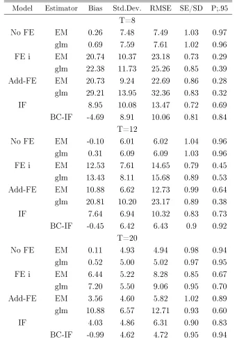
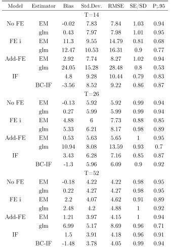
5 Simulations
empirical coverages of condence intervals with 95% nominal value (p; .95). All results are based on 500 replications.
The data generating processes are:
• DGP-1: Yit=1{Xitβ+εit>0}, (i= 1, ..., N; t= 1, ..., T),
• DGP-2: Yit=1{Xitβ+αi+εit>0}, (i= 1, ..., N; t = 1, ..., T),
• DGP-3: Yit=1{Xitβ+αi+γt+εit>0}, (i= 1, ..., N; t = 1, ..., T),
• DGP-4: Yit=1{Xitβ+αiγt+εit >0}, i= 1, ..., N; t= 1, ..., T,
where β = 1, αi ∼ N(0,1), γt ∼ N(0,1), and Xit ∼ N(0,1) are strictly exogenous with
respect to εit with εit ∼N(0,1).
Throughout, No FE refers to the probit without xed eects; FE i refers to the probit with individual xed eects; FE 2 refers to the probit with additive individual and time xed eects; IF refers to the probit with interactive xed eects; glm refers to the GLS estimator in R, while EM refers to the xed eects EM-type estimators proposed. For interactive xed eects, I also implement the bias correction procedure proposed here; BC-IF refers to the bias-corrected estimator. All the results are reported in percentages of the true parameter value.
The simulation results are summarized in Table 1 for N = 100 and T = 8,12,20, and
in Table 2 for N=52 and T = 14,26,52. They show that in all the cases analyzed EM has
smaller biases and variances and compares favorably to glm. For example, for the case with additive individual and time eects, when N = 100 and T = 12, the bias for glm is 21%,
whereas the EM estimator is only 11%. Even for the case without unobserved eects, when
N = 100andT = 20, the bias for glm is 0.52%, whereas the EM estimator is only 0.11%. In
terms of RMSE, for the case of individual eects, when N = 52 and T = 14, the RMSE for
6 Conclusion
This paper presents an EM-type method of estimating nonlinear panel data models with multiple unobserved eects, allowing for interactions between the unobserved individual and time specic eects. The method can be applied to models with individual eects, ad-ditive individual and time eects, interactive eects and other general functional form of unobserved eects. In nite-sample simulations, the method outperforms the existing iter-ative generalized least square methods for the models with individual eects and additive individual and time eects in terms of both bias and variance. Furthermore, I derive the asymptotic distribution of the proposed EM estimator for the panel probit model with in-teractive xed eects. Analytical bias corrections are developed to deal with the incidental parameter problem for both the estimates of the coecients and their associated average partial eects. Simulations demonstrate the correction works well in reducing the bias and root mean squared error and improves coverage rates. A wide range of future empirical and theoretical work can build upon the results of this paper. For example, sample selection models with interactive eects (for example, the international trade networks to control for other unobserved part that may aect certain factors on the likelihood of trade) or models with strategic interactions, such as binary game models, could benet from and build on the approach proposed here.
References
Ahn, S., Y. Lee, and P. Schmidt (2001): GMM estimation of linear panel data models with time-varying individual eects, Journal of Econometrics, 101, 219255.
(2013): Panel data models with multiple time-varying individual eects, Journal of Econometrics, 174, 114.
Andrews, D. (2005): Cross-section Regression with Common Shocks, Econometrica, 73, 15511585.
Arellano, M. and J. Hahn (2007): Understanding bias in nonlinear panel models: Some recent developments, Econometric Society Monographs, 43, 381.
(2009): Panel data models with interactive xed eects, Econometrica, 77, 1229 1279.
Bai, J. and S. Ng (2002): Determining the number of factors in approximate factor models, Econometrica, 70, 191221.
Bester, A. and C. Hansen (2009): Identication of marginal eects in a nonparametric correlated random eects model, Journal of Business & Economic Statistics, 27.
Bonhomme, S. (2012): Functional dierencing, Econometrica, 80, 13371385.
Carro, J. (2007): Estimating dynamic panel data discrete choice models with xed eects, Journal of Econometrics, 140, 503528.
Chamberlain, G. (1980): Analysis of Covariance with Qualitative Data, The Review of Economic Studies, 47, 225238.
Charbonneau, K. (2012): Multiple xed eects in nonlinear panel data models, Manuscript.
Chen, M., I. Fernández-Val, and M. Weidner (2013): Interactive xed eects in nonlinear panel data models with large N, T, .
Cunha, F. and J. Heckman (2008): Formulating, identifying and estimating the tech-nology of cognitive and noncognitive skill formation, Journal of Human Resources, 43, 738782.
Cunha, F., J. Heckman, and S. Schennach (2010): Estimating the technology of cognitive and noncognitive skill formation, Econometrica, 78, 883931.
Dempster, A., N. Laird, and D. Rubin (1977): Maximum likelihood from incomplete data via the EM algorithm, Journal of the Royal Statistical Society. Series B (Method-ological), 138.
Dhaene, G. and K. Jochmans (2010): Split-panel jackknife estimation of xed-eect models, Working paper.
Fernández-Val, I. (2009): Fixed eects estimation of structural parameters and marginal eects in panel probit models, Journal of Econometrics, 150, 7185.
Fernández-Val, I. and F. Vella (2011): Bias corrections for two-step xed eects panel data estimators, Journal of Econometrics, 163, 144162.
Fernández-Val, I. and M. Weidner (2014): Individual and Time Eects in Nonlinear Panel Data Models with LargeN, T, .
Freyberger, J. (2012): Nonparametric panel data models with interactive xed eects, Manuscript.
Gourieroux, C., A. Monfort, E. Renault, and A. Trognon (1987): Generalised residuals, Journal of Econometrics, 34, 532.
Greene, W. H. (2003): Econometric Analysis, Pearson Education India.
(2004): The behavior of the xed eects estimator in nonlinear models, The Econo-metrics Journal, 7(1), 98119.
Hahn, J. and G. Kuersteiner (2002): Asymptotically unbiased inference for a dynamic panel model with xed eects when both n and T are large, Econometrica, 70, 16391657.
(2011): Bias reduction for dynamic nonlinear panel models with xed eects, Econo-metric Theory, 27, 1152.
Hahn, J. and W. Newey (2004): Jackknife and analytical bias reduction for nonlinear panel models, Econometrica, 72, 12951319.
Heckman, J. J., J. Stixrud, and S. Urzua (2006): The Eects of Cognitive and Noncognitive Abilities on Labor Market Outcomes and Social Behavior, Journal of Labor Economics, 24, 411482.
Helpman, E., M. Melitz, and Y. Rubinstein (2008): Estimating Trade Flows: Trading Partners and Trading Volumes, The Quarterly Journal of Economics, 123, 441487.
Holtz-Eakin, D., W. Newey, and H. Rosen (1988): Estimating vector autoregressions with panel data, Econometrica, 56, 13711395.
McLeish, D. (1974): Dependent central limit theorems and invariance principles, Annals of Probability, 2, 620628.
Meng, X.-L. and D. Rubin (1993): Maximum likelihood estimation via the ECM algo-rithm: A general framework, Biometrika, 80, 267278.
Moon, H. R., M. Shum, and M. Weidner (2014): Estimation of random coecients logit demand models with interactive xed eects, Manuscript.
Moon, H. R. and M. Weidner (2010a): Dynamic linear panel regression models with interactive xed eects, Manuscript, University of Southern California.
(2010b): Linear regression for panel with unknown number of factors as interactive xed eects, Manuscript, University of Southern California.
Neyman, J. and E. Scott (1948): Consistent estimates based on partially consistent observations, Econometrica, 16, 132.
Orchard, T. and M. Woodbury (1972): A missing information principle: theory and applications, in Proceedings of the 6th Berkeley Symposium on mathematical statistics and probability, University of California Press Berkeley, CA, vol. 1, 697715.
Pan, J. (2002): The jump-risk premia implicit in options: Evidence from an integrated time-series study, Journal of Financial Economics, 63, 350.
Pastorello, S., V. Patilea, and E. Renault (2003): Iterative and recursive estimation in structural nonadaptive models, Journal of Business & Economic Statistics, 21, 449 509.
Pesaran, H. (2006): Estimation and inference in large heterogeneous panels with a mul-tifactor error structure, Econometrica, 74, 9671012.
A Results of Section 2
A.1 Panel probit with additive individual and time eects
In this setting, I consider the following model
Yit = 1{Yit∗ ≥0}, (11)
where all subjects are as dened previously.
Denition A.1. The xed eect EM estimator for panel probit with additive xed eects is dened by
(1) Given initial (β(k), α(k) i , γ
(k)
t ), denote µ (k) it =X
0
itβ(k)+α (k) i +γ
(k) t ,
(2) E-step: Calculate
ˆ
Yit(k) =µit(k)+ (Yit−Φ(µ (k)
it ))·φf(µ (k)
it )/{Φ(µ (k)
it )(1−Φ(µ (k) it )},
(3) M-step: This contains three conditional maximization steps CM-step 1: Given αi and γt, the parameter β can be updated by
β(k+1) = (
N
X
i=1 T
X
t=1
XitX
0
it)
−1{ N
X
i=1 T
X
t=1
Xit( ˆY (k) it −α
(k) i −γ
(k) t )},
CM-step 2: Given β and γt, the parameter αi can be updated by
αi(k+1) = 1
T
T
X
t=1
( ˆYit(k)−Xit0β(k+1)−γ(tk)),
CM-step 3: Given β and αi, the parameterγt can be updated by
γt(k+1) = 1
N
N
X
i=1
( ˆYit(k)−Xit0 β(k+1)−α(ik+1))
(4) Iterate until convergence.
Note that the CM-step 2 and CM-step 3 here are just the average over time and individual using Yˆ(k)
it as surrogate for Y
∗
it.
A.2 Proof of Proposition 2.1
By second-order Taylor expansion, for any two arguments θ1 and θ2,
−logF(θ1) = −logF(θ2)−
∂logF(θ2)
∂θ2
(θ1−θ2)− 1 2
∂2logF(θ)
Denote h(θ) = −∂log∂θF(θ). Using the fact that −logF(qitzit) is strictly convex on (0,1)
for logit and probit, and simple calculation shows0<−∂2log∂2θF(θ)|θ∗ <1, one has
−logF(θ1)≤ −logF(θ2) +h(θ2)(θ1−θ2) + 1
2(θ1−θ2) 2,
by completing the square, this can be written as
−logF(θ1)≤ −logF(θ2) + 1
2(θ1−θ2+h(θ2)) 2−1
2h 2(θ
2).
Now substitute qit(Xit0β+α0iγt) for θ1 and qit(Xit0βe+αe0ieγt)for θ2, one has
−logF(qit(Xit0β+α
0
iγt)) ≤ −logF(qit(Xit0βe+αe0ieγt)−
1 2h
2
(qit(Xit0 βe+αei0γet))
+1 2((X
0
itβ+α
0
iγt)−(Xit0βe+αe0ieγt) +qith(qit(Xit0 βe+αe0ieγt)))2
sum over i and t to obtain the required results.
B Proofs of Section 3
B.1 Proof of Consistency for βˆP P IF
Proof of Lemma 3.1. The proof contains two steps. With a little abuse of notation, in this section I use βˆ to denote βˆP P IF which is the estimate of the EM procedure for panel
probit models.
Step 1. Denote qit = 2Yit−1, and zit = X
0
itβ +αiγt. I prove the consistence directly
from the likelihood functionLN T =P i,t
log Φ(qitzit).
For any θ1 and θ2, the following is an upper bound for the negative log-likelihood:
−log Φ(θ1) ≤ −log Φ(θ2)−
φf(θ2) Φ(θ2)
(θ1−θ2) + 1
2(θ1−θ2) 2
= −log Φ(θ2) + 1
2(θ1−θ2−
φf(θ2) Φ(θ2)
)2−1 2(
φf(θ2) Φ(θ2)
)2,
where φf(·) is the Gaussian density. Substitute qitzit for θ1 and qitezit for θ2, then
−log Φ(qitzit) ≤ −log Φ(qitezit) +
1
2(zit−ezit+qit
φf(qitzeit)
Φ(qitezit)
)2− 1 2(
φf(qitezit)
Φ(qitezit)
Note, from the proof here, one can also infer using zeit = zit + qit
φf(qitzeit) Φ(qitzeit)
= zit + Yit−Φ(zit)
Φ(zit)(1−Φ(zit))φf(qitzit)is a good next step approximation, as the quadratic loss is a surrogate
for the Bernoulli log-likelihood function.
Step 2. Denote the structural error (generalized residual) as eit = Yit
−Φ(zit)
Φ(zit)Φ(−zit)φf(qitzit).
Since the estimated parameters minimize the objective function, with equation (12) one has
0 ≥ LN T(β0, φ0)− LN T( ˆβ,φˆ) ≥ 2N T1 P i,t
[(z0
it−zˆit+eit)2 −e2it]. The consistency proof for βˆ
is equivalent to that for the linear regression model with interactive xed eects. In matrix notation, as in Section 4, the above inequality would be
1
N TT r(ee
0) ≥ 1
N TT r[(X( ˆβ−β
0) + ˆαˆγ−α0γ0−e)(X( ˆβ−β0) + ˆαγˆ−α0γ0−e)0]
≥ 1
N TT r[Mα0(X( ˆβ−β
0)−e)M ˆ
γ(X( ˆβ−β0)−e)0],
here the projection matrixMˆγ =IT−γˆ[ˆγ0γˆ]−1γˆ0 =IT−T1ˆγˆγ0, andMα0 =IN−α0[α0
0
α0]−1α00.
With Assumption 1 (iv), which says that no linear combination of the regressors converges to zero, even after projecting any factor γ, one has
| 1
N TT r(e
0
Mα0XkMˆγ)|
≤ 1
N T|T r(e
0
Xk)|+
1
N T|T r(e
0
Pα0XkPˆγ)|+
1
N TT r(e
0
XkPγˆ) + 1
N TT r(e
0
Pα0Xk)
≤op(1) +
3
N TkekkXkk=op(1),
here one uses 1
N TT r(Xe
0
) =op(1),kek=op( √
N T). In addition, the assumption N T1 T r(XX0) =
Op(1) is satised from the distributional assumption on the regressors above.
Under those, 0 ≥ ckβˆ−βk+op(1)kβˆ−β0k+op(1), from which it is concluded that
ˆ
β =β0 +o p(1).
B.2 Proofs of Theorems 3.1 and 3.2
In this section, the notations are following Fernández-Val and Weidner (2014) as I extend the results to the interactive eects case. I suppress the dependence on N T of all the
sequences of functions and parameters to lighten the notation, e.g. L for LN T and φ for
φN T. Let∂xf denotes the partial derivative off with respect tox, and additional subscripts
denote higher-order partial derivatives. Hence, S(β, φ) =∂φL(β, φ) the dimφ-vector as the