Accepted
Article
Fixed effect variance and the estimation of repeatabilities and
heritabilities:
Issues and solutions
Pierre de Villemereuil1, Michael B. Morrissey2, Shinichi Nakagawa3, and Holger Schielzeth4
1School of Biological Sciences, University of Auckland, Auckland, New Zealand,
2School of Evolutionary Biology, University of St Andrews, St Andrews, UK, KY16 9TH,
3Evolution and Ecology Research Centre, University of New South Wales, Sydney, NSW 2052,
Australia, [email protected]
4Population Ecology Group, Institute of Ecology, Friedrich Schiller University, Dornburger
Str. 159, 07743 Jena, Germany, [email protected]
December 8, 2017
Acknowledgements
We thank A.J. Wilson for sharing his unicorn example data for us to analyse. HS was supported
by an Emmy Noether fellowship from the German Research Foundation (DFG; SCHI 1188/1-1). SN
is supported by a Future Fellowship, Australia (FT130100268). MBM is supported by a University
Research Fellowship from the Royal Society (London).
Accepted
Article
Abstract
Linear mixed effects models are frequently used for estimating quantitative genetic parameters,
including the heritability, as well as the repeatability, of traits. Heritability acts as a filter that
determines how efficiently phenotypic selection translates into evolutionary change, while
repeata-bility informs us about the individual consistency of phenotypic traits. As quantities of biological
interest, it is important that the denominator, the phenotypic variance in both cases, reflects the
amount of phenotypic variance in the relevant ecological setting. The current practice of quantifying
heritabilities and repeatabilities from mixed effects models frequently deprives their denominator
of variance explained by fixed effects (often leading to upward-bias of heritabilities and
repeatabil-ities) and it has been suggested to omit fixed effects when estimating heritabilities in particular.
We advocate an alternative option of fitting models incorporating all relevant effects, while
includ-ing the variance explained by fixed effects into the estimation of the phenotypic variance. The
approach is easily implemented and allows optimising the estimation of phenotypic variance, for
example by the exclusion of variance arising from experimental design effects while still including
all biologically relevant sources of variation. We address the estimation and interpretation of
heri-tabilities in situations in which potential covariates are themselves heritable traits of the organism.
Furthermore, we discuss complications that arise in generalised and non-linear mixed models with
fixed effects. In these cases, the variance parameters on the data scale depend on the location of
the intercept and hence on the scaling of the fixed effects. Integration over the biologically relevant
range of fixed effects offers a preferred solution in those situations.
Keywords: heritability, linear mixed modelling, fixed effects, quantitative genetics
Introduction
Additive genetic variance, phenotypic variance, and their ratio, the heritability of a trait, are key
parameters in evolutionary quantitative genetics, because they allow the assessment of whether a
phe-notypic trait can evolve through natural and artificial selection (Falconer and Mackay, 1996; Lynch
and Walsh, 1998). The heritability, h2, of a trait corresponds to the fraction of the selection differ-ential that can cause genetic change in the offspring generation. The heritability acts as a filter that
determines how efficiently a population can respond to phenotypic selection. Therefore, heritability is
relevant to assess the adaptive potential (e.g. in species threatened by global change (Hoffmann and
Sgr`o, 2011; Alberto et al., 2013)), as well as to investigate fundamental issues in evolutionary biology
(Mousseau and Roff, 1987; Meril¨a and Sheldon, 2000; Kruuk et al., 2000; Hadfield et al., 2006). A
Accepted
Article
example, to describe the individual consistency in phenotypic traits such as behaviour. Repeatability
can be used in a variety of context, but for the purpose of simplicity we here focus on individual
consistency, which is arguably the most widespread application in evolutionary ecology.
Mathematically, the heritability (and repeatability) of a trait are defined as the ratio of its additive
genetic variance VA (between-individual varianceVI) to its total phenotypic variance VP:
h2= VA
VP
, (1a)
R= VI
VP
, (1b)
As a measure of biological interest, heritability and repeatability should be estimated with the
eco-logically relevant phenotypic variance in the denominator, just as VA and VI should be estimated accounting for various confounding effects (Wilson et al., 2010) and in the relevant environment, since
genotype-by-environment (or individual-by-environment) interactions are common (Falconer, 1952;
Kawecki and Ebert, 2004; Stinchcombe, 2014). The phenotypic variance VP could ideally be quanti-fied by random sampling from the base population in a biologically relevant setting. But studies are
often designed, for good reasons, primarily for estimating VA and/or VI without bias and with the highest possible precision. Optimal sampling for the estimation of these variances can sometimes
gen-erate conflicts between the precise estimation of the numerators and the denominators of Eq. 1a. To
cope with these design choices, as well as to model experimentally and naturally arising confounding
effects, quantitative genetic models have to be as thorough as possible in terms of covariates accounted
for. This thoroughness inevitably leads to much complexity in the types and forms of effects included
in the model, which in turns might render the computation of some parameters, especially VP, more difficult than usually appreciated. As the two cases of heritability and repeatability have common
issues regarding the correct estimation of VP and the models to estimate heritability are generally slightly more complicated, we will focus on heritability throughout this article, but most arguments
apply to repeatability estimation as well.
The most popular methods for estimating quantitative genetic parameters make use of the linear
mixed models (LMM) framework (Kruuk, 2004; Wilson et al., 2010). In particular the so-called animal
model (Thompson, 1976), a special case of a mixed effects model, is widely used in plant and animal
breeding (Gianola and Rosa, 2015) and has been increasingly used in wild population studies over
Accepted
Article
accounting for various confounding effects (Kruuk, 2004; Wilson et al., 2010). A LMM fitted to explain
a phenotypey can contain both fixed and random effects and is conventionally written as:
y=µ+Xb+Zaa+Zu+e, (2)
where y is the vector of phenotypes y, µ is the global intercept and eis a vector of residual errors. TheXbpart stands for fixed effects (although not the intercept in the notation that we use here and
in the following), whereas Zu refers to the random effects. Random effects, unlike fixed effects, are
modelled as stemming from a normal distribution with a mean of zero and a variance to be estimated
from the data. Because of the quantitative genetic context discussed here, we isolate the random
effect Zaa corresponding to the additive genetic value of the individuals from other random effect
components. The matrices X and Z are referred to as the design and incidence matrices for the
fixed and random effects, respectively. Especially, theX matrix contains the values of the co-factors
included in the analysis. The vectors b and u contain the fitted fixed and potential random effect
estimates, respectively.
When no fixed effects (apart from the intercept µ) are included in the analysis, the heritability is simply calculated as:
h2= VA
VA+VRE+VR
, (3)
where VA stands for the variance in additive genetic values a, VRE for (the sum of) any relevant, i.e. accounting for natural sources of variation, additional random effect variance(s) and VR for the residual variance. Since variance decomposition using LMM separates the phenotypic variance into
additive components, Eq. 3 will generally give an unbiased estimate of Eq. 1a. Fixed effects, however,
can be problematic for multiple reasons.
Substantial progress has been made in highlighting issues pertaining to fixed effects in quantitative
genetic inferences (Wilson et al., 2010; Wolak et al., 2015), generating solutions for mixed model
analysis in general (Nakagawa and Schielzeth, 2013), and in data-scale quantitative genetic inference
using generalised mixed models (Nakagawa and Schielzeth, 2010; de Villemereuil et al., 2016). The
purpose of this paper is to synthesise the ideas in these previous works so as to provide an accessible
guidance to about what issues arise, and how to handle them, in a number of circumstances that are
Accepted
Article
P
henotypic
va
riation
Phenotypic trait
Fixed-e
ff
ect predictor
Rando
m
va
riation
V
ariation a
rising
fr
om f
ixe
d-e
ff
ect
Figure 1: Schematic description of an analysis using a continuous fixed-effect predictor to model a phenotypic trait, possibly with random effects. The graph shows the relationship between the fixed-effect predictor and the phenotypic trait (individual data points in black circles, values predicted by the model as black thick line). The total phenotypic variation (black double-arrow on the right) is decomposed into the fraction explained by fixed-effect variation (i.e. the phenotypic variation “along” the predicted model, in green) on one hand, and random variation (i.e. variation from random effects and residual error arising “around” the predicted model, in red) on the other hand.
Phenotypic variance estimation in the presence of fixed effects
Fixed effects are often fitted with the intention to account for confounding effects and improve the
goodness-of-fit of the models by accounting for complex patterns in the data. As illustrated in Fig. 1,
the variance of the random effects, as well as the residual variance are estimatedaround the predicted
values. Because of this, the sum of random variances (including additive genetic, random effects and
residual variances) underestimatesVP, as it does not reflect the total phenotypic variance of the trait, but rather the variance after the fixed effects have been accounted for (i.e. related to the red part in
Fig. 1).
As a consequence, fixed effects change the size of the phenotypic pie that is decomposed in different
components, if the denominator is calculated as in Eq. 3. Wilson (2008) recommended particular care
when fitting fixed effects in animal models and argued for a supplementary analysis without fixed
effects. Note that the issues tackled here and by Wilson (2008) about reduction of the denominator
variance when accounting for fixed effects also apply to the practice of two-step analyses by first fitting
a linear model to account for confounding effects and then analysing the heritability of the residuals
Accepted
Article
Since it will typically not be possible to get a benchmark for VP from an independent dataset, we need solutions that allow a reconstruction of VP in the presence of fixed effects. A simple solution would be to replace the denominatorVA+VRE+VR by the phenotypic variance in the original dataset
VPo, such that:
h2 = VA
VPo
. (4)
VPo will however be affected by various aspects of the experimental design and may not be represen-tative of the phenotypic variance in the base population (even if biases may be small in some cases of
well-balanced experimental designs).
A more proper solution is to account for the amount of variance that has been transferred from the
random components to the fixed effects. The variance VF arising from the fixed effect covariates will be the variance of the values predicted by the model (green part of Fig. 1) along all possible values for
the fixed-effect predictor (x-axis in Fig. 1). If we note ˆy the predicted value of the model according to a some specific predictor(s) value(s) and fx the distribution of the fixed-effect predictor(s), the
variance of fixed effects is thus the variance of ˆy along the distribution fx:
VF =
Z
Vx(ˆy)dfx, (5)
where Vx is the squared deviation from the mean (along the distribution fx). In practice, however,
a distribution fx of the covariates will not be known, as such distributions are not part of the linear
modelling assumptions. In the context of computing the coefficient of determination, Nakagawa and
Schielzeth (2013) proposed constructing a fixed effect variance component as the variance of the linear
predictor of the model yˆ =Xˆb. In other words, ˆy are the data points projected on the black thick
line in Fig. 1 and their corresponding varianceVF (i.e. related to the green part in the figure) can be computed as:
VF =V(ˆy) =V(Xˆb), (6) which is much simpler to compute than Eq. 5. When including this variance component in the
heritability calculation, the denominator is no longer sensitive to the presence and number of fixed
effects, because the variance transferred from random components to the fixed effects is now accounted
for in the new component VF (again, see Fig. 1 for a graphical illustration thatVP includes VF):
h2 = VA
VA+VF+VRE+VR
Accepted
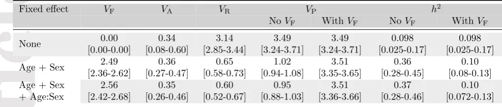
[image:7.595.33.544.147.256.2]Article
Table 1: Re-analysis of the unicorn dataset from Wilson (2008) in MCMCglmm (Hadfield, 2016), using models 1a, 1b and 1c from this reference (posterior mean of the estimates and 95% credible interval in bracket). We computed VF and provide VP and h2 with or without accounting for this component. Discrepancies in values fromh2 compared to Wilson (2008) are due a typological error in this reference (A.J. Wilson, personal communication).
Fixed effect VF VA VR VP h2
NoVF WithVF NoVF WithVF
None 0.00 [0.00-0.00] 0.34 [0.08-0.60] 3.14 [2.85-3.44] 3.49 [3.24-3.71] 3.49 [3.24-3.71] 0.098 [0.025-0.17] 0.098 [0.025-0.17]
Age + Sex 2.49 [2.36-2.62] 0.36 [0.27-0.47] 0.65 [0.58-0.73] 1.02 [0.94-1.08] 3.51 [3.35-3.65] 0.36 [0.28-0.45] 0.10 [0.08-0.13] Age + Sex
+ Age:Sex 2.56 [2.42-2.68] 0.35 [0.26-0.46] 0.60 [0.52-0.67] 0.95 [0.88-1.03] 3.51 [3.36-3.66] 0.37 [0.28-0.46] 0.10 [0.072-0.13]
This is a straightforward calculation that can be applied for any analysis, and using most software,
since it needs only the values of the co-factors (i.e. the design matrixX) and the parameter estimates.
The former is an aspect of the sampling and/or experimental design and the latter is part of the
output of any statistical software. The computation of repeatability using VF is straightforward by replacingVAby VIin Eq. 7, as in Eq. 1b.
It will be useful to provide estimates of this component in publications, in order to reflect how
much variance was depleted because of the presence of fixed effects. The same kind of solution could
be applied if the heritability was measured on the residuals of a regression (sometimes referred to as
“corrected phenotypic values”): the variance of the regression model (VF, following the exact same definition as in Eq. 6) could be computed and included inVP, though a better practice anyway would be to run everything within a single LMM.
As an illustration, we re-analysed the unicorn example data from Wilson (2008) using the
MCM-Cglmm R package (Hadfield, 2016). This analysis of unicorn horn length (Table 1) shows that
ac-counting for the VF component allow to recover the correct value forVP and hence for h2, whichever the structure of the fixed effect component. Hence, because this practice would answer the concerns
raised by Wilson (2008), we encourage researchers to include fixed effects in their analyses. A decision
not to fit influential fixed effects, despite their beneficial effect on the goodness-of-fit or for accounting
for confounding effects, would likely harm model fit, parameter estimation and possibly the behaviour
of the test statistics. Improving the fit of the model would most likely improve the precision of the
estimates, which, for any particular dataset, would improve the precision of the heritability estimate
(the point estimate would be more probably close to its true value and the confidence interval will be
Accepted
Article
confounded with the additive genetic component VA (e.g. common environment effects) are likely to reduce upward bias in the heritability estimate and will tend to result in lower, but more accurate
point estimates of heritabilities.
Table 2: Fixed effects literature survey. This literature survey does not claim completeness, but should be representative for heritability estimates in wild population using the animal model.
R´ef´erence Nb. effects Fixed effects
Natural variation Experimental variation
R´eale et al. (1999) 2 Sex, Years —
Kruuk et al. (2000) 2 Age, Area —
Milner et al. (2000) 8
Age, Parasite burden, Birth Year, Year of measurement, Birth type, Coat color, Horn type
Catch date
Kruuk et al. (2001) 1 — Brood size manipulation Meril¨a et al. (2001) 1 — Brood size manipulation
Kruuk et al. (2002) 1 Age —
MacColl and Hatchwell (2003) 6 Year, Sex, Helper, Hatch date,
Area, Attempt —
Sheldon et al. (2003) 1 Year —
Hadfield et al. (2006) 5 Sex, Year, Hatch date Carotenoid treatment, Immune treatment Th´eriault et al. (2007) 4 Age, Year Day of capture
Nilsson et al. (2009) 3 Age, Dyad Brood size manipulation Morales et al. (2010) 3 Eggmass, Age Treatment
Charmantier et al. (2011) 2 Sex, Natal colony —
Doligez et al. (2011) 2 Sex, Age —
Lane et al. (2011) 2 Age-class, Year —
Reid et al. (2011b) 1 Year —
Reid et al. (2011a) 2 Year, Age-class —
Evans and Sheldon (2012) 3 Sex, Age Measurement day B´er´enos et al. (2014) 3 Sex, Litter size Age at capture
Lane et al. (2015) 4 Age, Cone availability, Litter
size, Year —
Removing the influence of experimental design on
V
PIn the context of estimating the phenotypic variance of a trait, fixed effects (as well as random effects)
may be of two kinds. They can either reflect natural sources of variation that we are interested
in, or variance arising from experimental and/or design effects. Since the latter category artificially
inflates the variance in the data, we might wish to exclude this source of variance from the heritability
calculation. For example, if we want to study the amplitude of insect songs in the field, we might
want to improve our model fit by including effects accounting for natural sources of variation, such
Accepted
Article
design, such as the distances between the animal and the microphone. Yet, in the computation of the
phenotypic variance VP, we might want to include the biological variance arising from age, but not the experimental variance arising from the distance.
We have categorised fixed effects in a cursory literature survey (Table 2) into sources of natural or
experimental variation for illustration. Most of the fixed effects included in these analyses originate
from natural variation (e.g. sex, year, age, area, litter size) and most likely should be included in
VP. Others are of experimental origin either being an experimental treatment or of design origin (e.g. due to variation in the time of measurement) and should probably be excluded from VP. Of course, this separation between natural and experimental sources of variation can be quite difficult
(e.g. year of sampling may represent error measurement or relevant natural variation depending on
context). Furthermore, it can sometimes be interesting to also exclude natural sources of variation.
For example, “age” or “sex” could be excluded from the denominator to get heritabilities conditional
on those factors. This would allow performing evolutionary prediction for a particular age-class or
sex.
In essence, what is required is to compute the phenotypic variance including the “natural” factors
xnat conditional on the experimental factorsxexp:
VF=
Z
Vx(ˆy|xexp)dfxnat|xexp(xnat). (8)
To exclude the particular factor(s) in practice, the predictor(s) (i.e. the respective columns in the
design matrix) and the related inferred parameters can simply be left out of a new linear predictorˆy?
in the calculation of VF such that:
VF =V(ˆy?). (9)
This is equivalent to Eq. 8, in the sense that it is accounting for the variance due to the factors included
in the computation of ˆy? conditional on the effect of other factors that have been excluded. Note, however, that this computation is unfortunately not general and is based on the assumptions that the
measured variance of the natural predictors is not caused by any of the experimental predictors. A
more general solution relies on path analysis and the assumption of a causal pathway between variables
(see Box 1).
A strong assumption in the equations above is that the sampled design matrixXfor the cofactors
Accepted
Article
case. For example, the insects that we are studying with respect to song amplitude might occur in
distinct morphotypes (and these morphotypes differ in song amplitude) that are not equally common.
For statistical reasons it may be useful to oversample rare morphs if we want to estimate the effect
of morph on song amplitude. Such a sampling design will equalize morph frequencies in the sample
and will thus tend to inflateVFif calculated asXˆb. Statistical requirements (balanced sampling) and biological realism (natural morph ratios) differ in this case and the calculation should account for this
difference, especially we need to ensure the denominator actually reflect natural variation. A solution
is to use Eq. 5 directly by assuming a distributionfx for our morphotypes.
Although this might be feasible in this simple example, it will be more difficult as soon as many
covariates have to be included, for which a joint distribution must be assumed. Two other solutions are
possible. One possible solution would be to use Eq. 6, but replace the design matrixX by a modified
design matrix X0 that more closely matches the distribution of covariates to the natural population
variation (e.g. sampled observations from the field) to compute the predicted values (noted ˆy0).
Note that, when constructingX0, we should still take into account potential correlations between
co-factors. For example if the rare morph is preferentially present in warm environments and temperature
is included in the model, thenX0 should reflect that correlation. Additionally, the computation ofX0
will only represent a possible sampling of the true population, thus this solution will come with the
drawback of sampling noise arising form this.
Another possible solution would be to use a slightly different (but exactly equivalent) approach
compared to Eq. 6 and computeVFas the product between the variance of the covariate in the natural population and their squared estimated effects. For a model with a simple continuous covariatexwith
an associated slope ˆbx, this will be:
VF = ˆb2xV(x) (10)
For a multivariate model, the variance-covarianceS0 of the covariates in the wild population is required
(and can be easily computed from raw data) and one can compute VF in the multivariate analogous of Eq. 10:
VF =ˆb|S0bˆ, (11) where|is the symbol for the transpose operation. The main advantage of this solution (again, exactly
equivalent as the above approach) is that, compared to the resampling of a design matrix X0, it does
Accepted
Article
data collection on the natural population and model estimates). All the issues and solutions discussed
here equally apply to the computation of repeatability.
Fitting of genetic covariates and implicit assumptions about genetic
covariances
A general consideration is whether fixed effects should cover only non-genetic sources of variation.
Morphs in our example might be environmentally or genetically determined and it is usually advisable
to model such discrete effects with potentially oligocausal control as fixed effects, no matter whether
they are ultimately genetic or environmental in origin. With purely monogenic inheritance of morphs,
morph phenotype is essentially a genetic marker for a (potential) quantitative trait locus (QTL) and
thus represents the local heritability in linkage with the morph-determining locus (see e.g. Payne,
1918; Sax, 1923, for early QTL studies using Mendelian phenotypes as markers), while the polygenic
contribution of the background is captured by VA. Whether or not covariates cover genetic or non-genetic effects matters for the interpretation, since the estimate of VA (and consequently h2) might represent the total VA or the background VA other than the local heritability at the QTL.
Some potential covariates might also be (heritable) polygenic traits themselves. In many cases,
relationships between a heritable focal trait and some other relevant heritable trait are best handled
with multi-response models (see Hadfield, 2010; Wolak et al., 2015), wherein the potential covariate
is treated as a response along with the focal trait. Such a model estimates the genetic (and
non-genetic) variances for both traits along with genetic (and non-non-genetic) covariances among the traits
treated as responses. This is not the case when the potential covariate is fitted as a fixed effect in
the model: the fixed effect will explain the total influence of the covariate on the focal trait but not
explicitly distinguish between (nor differentially estimate) different sources of covariances. There are
situations where it does make sense to include polygenic traits as fixed covariates, particularly when
studying questions where causal effects of traits on one another are relevant. Further discussions of
such scenarios are presented in Gianola and Sorensen (2004) and Morrissey (2014, 2015).
To illustrate this, let us go back to Wilson (2008)’s unicorn dataset. It is a known fact that
in unicorns, horn length varies according to the individual body mass (slope: β = 0.403 for a full model including age, sex and their interaction). It would thus seem relevant to add body mass
Accepted
Article
heritability (accounting forVF) ofh2horn length|body mass= 0.066 (Table S1 in Appendix). This is slightly lower than the estimate in Table 1, despite the fact that we accounted for the variance explained by
the fixed effects. Yet, the inferred phenotypic variance (VP,horn length|body mass = 3.47, Table S1) is comparable to the estimate in Table 1, what is now different is the estimate of the additive genetic
variance (VA,horn length|body mass= 0.23, Table S1, lower thanVA,horn length= 0.35 in Table 1). What is causing this lower additive genetic variance? Incidentally, we also know that body mass is a heritable
trait (VA,body mass = 0.328 and h2body mass = 0.344, Table S2). Moreover, a bivariate model shows that it is genetically correlated with horn length (rG = 0.63, Table S3). Hence, by including body mass as a fixed effect, we have been “explaining away” some of the additive genetic variance of
horn length, precisely because of this genetic correlation. A naive way to obtain a correct estimate
of the additive genetic variance of horn length, without resorting to a bivariate model, would be
to use the slope of the regression of horn length on body mass and compute the additive genetic
variance as VA,horn length|body mass+β2VA,body mass = 0.23 + 0.162×0.328 = 0.283, which doesn’t quite restore VA,horn length to its original value. This is because this computation use the total slope of the relationship between horn length and body mass, hence assuming an effect of the phenotypic value of
body mass on the genetic value of horn length, which is apparently not a good assumption here. Any
more accurate recovery ofVAwill almost always require to fit a bivariate model. Because of the issues highlighted here, we believe it is advisable, whenever possible, to fit multivariate models between
heritable and putatively genetically correlated traits instead of using other traits as covariates.
More generally, whether the covariate variability is of genetic or environmental origin, we still
make an implicit strong assumption about the structure of genetic variation of the response trait(s).
In particular, we assume that the additive genetic effects (and especially their variance) are constant
across the range of the covariate or categorical factor. In doing so, we assume that
genotype-by-covariate interactions are negligible, or put differently, that there is a perfect genetic correlation e.g.
between categories of the categorical covariate. This assumption is frequently violated. In the special
case of sex, for example, it has been shown that fitting sex as a fixed effect in a LMM leads to
(downward) biased estimates unless the cross-sex genetic correlation is perfect (Wolak et al., 2015).
Note that repeatability might also be impacted by the inclusion of biological covariates that are
themselves repeatable and share some of the underlying mechanisms of this repeatability (e.g. genetics
Accepted
Article
Non-linear models and non-Gaussian traits
The influence of fixed effects becomes more complex, and thus even more important to consider
carefully, when the data are non-linear in the parameters of a model. Such non-linearity arises in
linear mixed models (NLMMs), in generalised linear mixed models (GLMMs), through the
non-linearity of their link functions, and when data are non-linearly transformed prior to analysis. In
GLMMs, a distinction is critical between the latent scale and the data scale (Morrissey et al., 2014):
on the former, we assume linearity, normality and perform most of the inferences, whereas the latter
is a non-linear transformation from the latent scale (e.g. through the link function). Hence, the
above framework could be used to compute heritabilities and repeatabilities on the linear, normally
distributed, latent scale, but creates difficulties with methods transforming estimates from the latent
scale to the data scale (see e.g. Table 1 and 2 in Nakagawa and Schielzeth, 2010).
Non-linearity causes dependence between fixed and random effects, with the direct consequences
that quantitative genetic parameters can no longer be computed without accounting for the whole
distribution of fixed effects. In other words, in a GLMM, variation associated with fixed effects does
not only potentially contribute to the phenotypic variance, but the contribution to the phenotypic
variance is not constant across the distribution of fixed effects (de Villemereuil et al., 2016). HenceVA and VP on the data scale become complex functions of all the parameters. This means that adding a
VF component to the computation of VP will not work any longer, because the additivity of the fixed effects and random effects variance components is not valid in these models. De Villemereuil et al.
(2016) showed that we need to integrate over the predicted values based on fixed effects to compute
quantitative genetic parameters using a GLMM. The same logic applies when working with non-linear
models or with data that was non-linearly transformed, unless we are specifically interested in the
heritability of the transformed data.
Alastair Wilson collected data on the number of aggressive behaviours performed in a single day
on all unicorn individuals for which he analysed the genetics of horn length in his 2008 paper. Here,
we conduct analyses of these data to illustrate how, in addition to h2, variance components such as
VAand VP depend on the full distribution of fixed effects. Fig 2 show how, according to our Poisson GLMM model, the effect of the sex covariate impacts the observed number of aggressive behaviours:
despite the two sexes having the same variance in their latent values and differing only in mean latent
value (males having larger values, with little overlap), the counts of aggressive behaviours do not
Accepted
Article
−0.5 0 0.5 1 1.5 2 2.5 0 0.25 0.75 1
0 0.5 1 1.5
0
1
2
3
4
5
6
7
8
9
10
11
12
latent scale value data scale
distribution
latent density
obser
v
ed v
alue
inverse link function
females males
Accepted
Article
Latent scale Intercept VF VR VA
Variances 0.0871
(-0.0533 - 0.254)
0.307 [0.273 - 0.342]
0.0973 [0.0686 - 0.13]
0.0317 [0.00766 - 0.056]
Observed scale Mean VA,obs VP,obs h2obs
(i) Using the intercept
1.17 (0.984 - 1.35)
0.0434 (0.0114 - 0.0813)
1.36 (1.14 - 1.61)
0.0318 (0.00825 - 0.0564)
(ii) Adding VF (1.16 - 1.55)1.36 (0.0154 - 0.11)0.0589 (1.95 - 2.79)2.37 (0.00722 - 0.0447)0.0247
(iii) Integrating over predictions
3.49 (3.37 - 3.62)
0.386 (0.113 - 0.709)
10.3 (9.3 - 11.4)
0.0377 (0.0119 - 0.0695)
Table 3: Results of fitting a model for number of observed aggressive behaviours using a Poisson distribution in MCMCglmm. First row: estimate of the intercept of the model and variance decom-position on the latent scale. Three last rows: estimates of population mean, additive genetic variance, phenotypic variance and heritability computed on the observed data scale using QGglmm(i) ignoring fixed effect and only providing the intercept;(ii)providing the intercept but includingVFin the latent total variance or(iii) using the whole latent predicted values distribution.
with females). This non-linearity of the effects can be linked to two subsequent phenomenons. To
begin with, the exponential inverse link function assumed in the Poisson GLMMs is strongly
non-linear: this results in the fact that two pairs (one for female, one for male, see red and blue arrows)
of evenly spaced values on the latent scales are not evenly spaced after transformation through the
inverse link-function. On top of this, the variance of a Poisson distribution is equal to the mean:
this creates even more variance for large values (see dotted arrows and corresponding distributions of
aggressive behaviours for males and females). The strong effect of this non-linearity on the variances
of the phenotypic trait raises the question of how to best account for the variance “explained” by fixed
effects.
We analysed the number of aggressive behaviours using the R package MCMCglmm and a Poisson
family including sex, age and their interaction as fixed effects. The results of the analysis on the
latent scale (direct output from MCMCglmm) are available in the first row of Table 3. We can see
that the fixed effects account for a large part of the phenotypic variance (VF is larger than VA and
VR). Using the framework from de Villemereuil et al. (2016) implemented in the QGglmm R package, we then computed the quantitative genetic parameters on the observed data scale using three different
approaches: (i) not accounting for fixed effects at all, (ii) accounting the variance of fixed effects
in the total variance of the latent scale and (iii) using the whole distribution of predicted values to
Accepted
Article
accounting for the whole distribution of predicted values (last row) is the only approach that yields a
population mean and phenotypic variance compatible with the sample estimates (number of aggressive
behaviours, mean = 3.41 and variance = 9.77).
The analysis of unicorn aggression data illustrates that the approach of using a VF component suggested here can only be applied directly to phenotypic traits with a normal error distribution
and analysed using linear mixed models (or if the analysis is based on the latent scale of a GLMM).
However, solutions to integrate over the distribution of predicted values do exist, such as assuming a
distribution of the fixed-effect covariates (see Eq. 19 in de Villemereuil et al., 2016) or averaging over the
predicted values according the fixed effects (i.e. averaging overˆy) within the integral computation (see
Eq. 18 in de Villemereuil et al., 2016). This latter approach has been implemented in the QGglmm
R package. This approach of course assumes that the distribution of fixed effects in the sample is
representative for the base population of interest. Otherwise, the design matrices might need to be
adjusted accordingly (e.g. by providing a construct such as yˆ? or ˆy0 introduced above, or a mix of
these constructs, as the predicted values to QGglmm).
On this subject, it must be noted that repeatability and heritability are computed differently for
GLMMs as the narrow-sense heritability on the observed data scale of GLMMs is not an intra-class
correlation coefficient any more (see the difference between Eqs. 9 and 16 in de Villemereuil et al.,
2016).
Conclusion & Perspectives
Wilson (2008) identified an issue when fixed effects are included a quantitative genetic model: the
inclusion of fixed effects in the model has an influence on the computation of the phenotypic variance.
Based on recent work from several sources, we provide guidelines to overcome this and other related
issues, in the hope this will facilitate the use and interpretation of quantitative genetic mixed models
with fixed effects. We also discussed the complications arising from the diverse and complicated
nature of covariates that can be fitted as fixed effects. We think that fixed effects are an opportunity
to finely control confounding effects. Yet, when belonging to the phenotypic variance, they need to be
included in the denominator of the heritability and repeatability. In order to do so, we here promote
the practice of accounting for the “fixed-effect” variance componentVF(see Nakagawa and Schielzeth, 2013), which includes the variance of all or selected fixed effects to be added in the denominator
Accepted
Article
data (including how to implement Eqs. 9 and 11, see Supplementary Information) and the R package
MCMCglmm (Hadfield, 2016) to show how these calculations can be implemented and how they can
affect the output (h2 estimates changing from 0.66 when not includingVF in the denominator to 0.15 when including it in our example). The code for the analysis of the unicorn examples is also provided.
This approach has several advantages. First, it overcomes Wilson (2008)’s legitimate reluctance of
including fixed effects in the model. When includingVF in the denominator, there is no issue of “lost variance”. Second, since we are now able to include fixed effects, we have gained a finer control on
confounding effects on the additive variance. It also requires some careful consideration of which fixed
effects represent experimental design effects and which are biologically relevant. Third, it provides us
with the choice of whether or not to include effects inVF, depending on whether or not we deem them part of the natural phenotypic variance of the studied population. Fourth, as argued above for the
case of morphotypes in the context of song amplitude, the calculation of VF can accommodate some discrepancies between the analysed data and the actual population in the distribution of covariates.
Overall we advocate for the inclusion of fixed effects in linear mixed models to estimate heritabilities
and repeatabilities when (i) this improves the goodness-of-fit of the model and/or helps to account
for confounding effects and(ii) a carefully computed VF component is included in the calculation of the denominator. While this is generally also true for non-linear models and GLMMs, any model
that involves non-linearity in the response to fixed effects will require particular attention and likely
integration over their biologically relevant range in order to marginalize the influence of fixed effects.
Box 1: Using path analysis to obtain a partial VF
Path analysis Path analysis is a statistical analysis aiming at evaluating the directed influence of
variables onto others. This directed relationship is referred to ascausality (Wright, 1921). The direction
of the relationship has a strong influence in our case, because it allows us to predict if the presence of
one variable would inflate the variance of another.
Three examples In the figure below are three different examples using a phenotypic variable of
interestP influenced by a biological variable B and an experimental variableE. The parametersbXY
stand for the coefficient of a model of the effect of X onY (e.g. a slope). The parameters σX is the
exogenous standard-deviation of the variable X, i.e. its standard-deviation due to influences outside of
Accepted
Article
σXY is the exogenous covariance between X and Y, i.e. a undirected covariance arising from common
influences outside of the causal pathway or due to physical/logical constraints (e.g. size and volume are
physically covarying).
B
σB
σBE
E
σE
P
σP bBP bEP
1
B
σB bBEE
σEP
σP bBP bEP2
B
σB bEBE
σEP
σP bBP bEP3
General principle In all cases, we are only interested in computing the variance arising from the
grey area of the pathway (B and P), while excluding variance arising fromE. ExcludingE from the
graph means that we set its exogenous standard-deviation (σE) and possible covariances (e.g.σBE), as
well as all the coefficients of its effect on any variable (e.g. bEP), to zero. Given that, the “fixed-effect
variance” ofP in this graph excludingE is simply the variance arising from the effect ofB:
VF=b2BPσ
2
B
We will see that the difference between the three examples lies in the computation of σB.
Example 1 In this example, the variables B and E share an undirected covariance σXY. In other
words, we assume that a set of unmeasured variables have an effect on both B and E, but not that
a change in E will affectB. In that case, the exogenous variance of B is merely its actual variance:
σ2
B=V(B).
Example 2 In this example, the variableB has a direct effect onE (e.g. because an aspect of the
species biology modulate the effect of the experimental treatment). In that case, changes of variance in
Bwill affect the variance ofE, but this is not a problem for us since we want to excludeE. Once again,
the exogenous variance of Bis merely its actual variance: σ2
B=V(B).
Example 3 In this example however, the variableEhas a direct effect on the variableB(e.g. because
the experimental treatment has an effect over different parts of the biological system). This means that,
by experimentally introducingE into the biological system, we also experimentally increased the actual
variance of B. To compute the exogenous variance of B, we need to remove this additional variance:
σ2
B = V(B|E). In other words, σ
2
B is here the residual variance of a model of the effect of E on B
Accepted
Article
References
Alberto, F., Aitken, S. N., Al´ıa, R., Gonz´alez-Mart´ınez, S. C., H¨anninen, H., Kremer, A., Lef`evre, F.,
Lenormand, T., Yeaman, S., Whetten, R., and Savolainen, O. (2013). Potential for evolutionary
responses to climate change – evidence from tree populations. Global Change Biology, 19(6):1645–
1661.
B´er´enos, C., Ellis, P. A., Pilkington, J. G., and Pemberton, J. M. (2014). Estimating quantitative
ge-netic parameters in wild populations: a comparison of pedigree and genomic approaches. Molecular
Ecology, 23(14):3434–3451.
Charmantier, A., Buoro, M., Gimenez, O., and Weimerskirch, H. (2011). Heritability of short-scale
natal dispersal in a large-scale foraging bird, the wandering albatross. Journal of Evolutionary
Biology, 24(7):1487–1496.
de Villemereuil, P., Schielzeth, H., Nakagawa, S., and Morrissey, M. B. (2016). General methods for
evolutionary quantitative genetic inference from generalised mixed models. Genetics, 204(3):1281–
1294.
Doligez, B., Daniel, G., Warin, P., P¨art, T., Gustafsson, L., and R´eale, D. (2011). Estimation
and comparison of heritability and parent–offspring resemblance in dispersal probability from
cap-ture–recapture data using different methods: the Collared Flycatcher as a case study. Journal of
Ornithology, 152(S2):539–554.
Evans, S. R. and Sheldon, B. C. (2012). Quantitative Genetics of a Carotenoid-Based Color:
Her-itability and Persistent Natal Environmental Effects in the Great Tit. The American Naturalist,
179(1):79–94.
Falconer, D. S. (1952). The problem of environment and selection. The American Naturalist,
86(830):293–298.
Falconer, D. S. and Mackay, T. F. (1996). Introduction to quantitative genetics. Benjamin Cummings,
Harlow, Essex (UK), 4 edition.
Garland, T. (1988). Genetic Basis of Activity Metabolism. I. Inheritance of Speed, Stamina, and
Accepted
Article
Gianola, D. and Rosa, G. J. M. (2015). One hundred years of statistical developments in animal
breeding. Annual Review of Animal Biosciences, 3(1):19–56.
Gianola, D. and Sorensen, D. (2004). Quantitative genetic models for describing simultaneous and
recursive relationships between phenotypes. Genetics, 167(3):1407–1424.
Hadfield, J. D. (2010). MCMC methods for multi-response generalised linear mixed models: The
MCMCglmm R package. Journal of Statistical Software, 33(2):1–22.
Hadfield, J. D. (2016). MCMCglmm Course Notes.
Hadfield, J. D., Burgess, M. D., Lord, A., Phillimore, A. B., Clegg, S. M., and Owens, I. P. F. (2006).
Direct versus indirect sexual selection: genetic basis of colour, size and recruitment in a wild bird.
Proceedings of the Royal Society B: Biological Sciences, 273(1592):1347–1353.
Hoffmann, A. A. and Sgr`o, C. M. (2011). Climate change and evolutionary adaptation. Nature,
470(7335):479–485.
Kawecki, T. J. and Ebert, D. (2004). Conceptual issues in local adaptation. Ecology Letters,
7(12):1225–1241.
Kruuk, L. E., Clutton-Brock, T. H., Slate, J., Pemberton, J. M., Brotherstone, S., and Guinness, F. E.
(2000). Heritability of fitness in a wild mammal population. Proceedings of the National Academy
of Sciences, 97(2):698–703.
Kruuk, L. E., Meril¨a, J., and Sheldon, B. C. (2001). Phenotypic selection on a heritable size trait
revisited. The American Naturalist, 158(6):557–571.
Kruuk, L. E. B. (2004). Estimating genetic parameters in natural populations using the ‘animal
model’. Philosophical Transactions of the Royal Society of London. Series B: Biological Sciences,
359(1446):873 –890.
Kruuk, L. E. B., Slate, J., Pemberton, J. M., Brotherstone, S., Guinness, F., and Clutton-Brock, T.
(2002). Antler size in red deer: heritability and selection but no evolution. Evolution, 56(8):1683–
1695.
Lane, J. E., Kruuk, L. E. B., Charmantier, A., Murie, J. O., Coltman, D. W., Buoro, M., Raveh, S.,
and Dobson, F. S. (2011). A quantitative genetic analysis of hibernation emergence date in a wild
Accepted
Article
Lane, J. E., McAdam, A. G., Charmantier, A., Humphries, M. M., Coltman, D. W., Fletcher, Q.,
Gorrell, J. C., and Boutin, S. (2015). Post-weaning parental care increases fitness but is not heritable
in North American red squirrels. Journal of Evolutionary Biology, 28(6):1203–1212.
Lynch, M. and Walsh, B. (1998). Genetics and analysis of quantitative traits. Sinauer Associates,
Sunderland, Massachussets (US).
MacColl, A. D. C. and Hatchwell, B. J. (2003). Heritability of parental effort in a passerine bird.
Evolution, 57(9):2191–2195.
Meril¨a, J., Kruuk, L. E. B., and Sheldon, B. C. (2001). Natural selection on the genetical component
of variance in body condition in a wild bird population. Journal of Evolutionary Biology, 14(6):918–
929.
Meril¨a, J. and Sheldon, B. C. (2000). Lifetime reproductive success and heritability in nature. The
American Naturalist, 155(3):301–310.
Milner, J. M., Pemberton, J. M., Brotherstone, S., and Albon, S. D. (2000). Estimating variance
components and heritabilities in the wild: a case study using the ‘animal model’ approach. Journal
of Evolutionary Biology, 13(5):804–813.
Morales, J., Kim, S., Lobato, E., Merino, S., Tom´as, G., Mart´ınez de la Puente, J., and Moreno,
J. (2010). On the heritability of blue-green eggshell coloration. Journal of Evolutionary Biology,
23(8):1783–1791.
Morrissey, M. B. (2014). Selection and evolution of causally-covarying traits. Evolution, 68:1748–1761.
Morrissey, M. B. (2015). Evolutionary quantitative genetics of nonlinear developmental systems.
Evolution, 69(8):2050–2066.
Morrissey, M. B., de Villemereuil, P., Doligez, B., and Gimenez, O. (2014). Bayesian approaches to the
quantitative genetic analysis of natural populations. In Charmantier, A., Garant, D., and Kruuk,
L. E., editors, Quantitative Genetics in the Wild, pages 228–253. Oxford University Press, Oxford
(UK).
Mousseau, T. A. and Roff, D. A. (1987). Natural selection and the heritability of fitness components.
Accepted
Article
Nakagawa, S. and Schielzeth, H. (2010). Repeatability for Gaussian and non Gaussian data: a practical
guide for biologists. Biological Reviews, 85(4):935–956.
Nakagawa, S. and Schielzeth, H. (2013). A general and simple method for obtaining R2 from
gener-alized linear mixed-effects models. Methods in Ecology and Evolution, 4(2):133–142.
Nilsson, J.-A., ˚Akesson, M., and Nilsson, J. F. (2009). Heritability of resting metabolic rate in a wild
population of blue tits. Journal of Evolutionary Biology, 22(9):1867–1874.
Payne, F. (1918). The effect of artificial selection on bristle number in Drosophila ampelophila and its
interpretation. Proceedings of the National Academy of Sciences of the United States of America,
4(3):55.
Postma, E. (2014). Four decades of estimating heritabilities in wild vertebrate populations: Improved
methods, more data, better estimates. In Charmantier, A., Garant, D., and Kruuk, L. E. B., editors,
Quantitative genetics in the wild, pages 16–33. Oxford University Press, Oxford (UK).
Reid, J. M., Arcese, P., Sardell, R. J., and Keller, L. F. (2011a). Additive genetic variance,
heritabil-ity and inbreeding depression in male extra-pair reproductive success. The American Naturalist,
177:177–187.
Reid, J. M., Arcese, P., Sardell, R. J., and Keller, L. F. (2011b). Heritability of female extra-pair
paternity rate in song sparrows (Melospiza melodia). Proceedings of the Royal Society B: Biological
Sciences, 278(1708):1114 –1120.
R´eale, D., Festa-Bianchet, M., and Jorgenson, J. T. (1999). Heritability of body mass varies with age
and season in wild bighorn sheep. Heredity, 83(5):526–532.
Sax, K. (1923). The association of size differences with seed-coat pattern and pigmentation in
Phase-olus vulgaris. Genetics, 8(6):552.
Sheldon, B. C., Kruuk, L. E. B., and Merila, J. (2003). Natural selection and inheritance of breeding
time and clutch size in the collared flycatcher. Evolution, 57(2):406–420.
Stinchcombe, J. R. (2014). Cross-pollination of plants and animals: wild quantitative genetics and
plant evolutionary genetics. In Charmantier, A., Garant, D., and Kruuk, L. E., editors,Quantitative
Accepted
Article
Thompson, R. (1976). The estimation of maternal genetic variances. Biometrics, 32(4):903–917.
Th´eriault, V., Garant, D., Bernatchez, L., and Dodson, J. J. (2007). Heritability of life-history tactics
and genetic correlation with body size in a natural population of brook charr (Salvelinus fontinalis).
Journal of Evolutionary Biology, 20(6):2266–2277.
Wilson, A. J. (2008). Why h2 does not always equal VA/VP? Journal of Evolutionary Biology,
21(3):647–650.
Wilson, A. J., R´eale, D., Clements, M. N., Morrissey, M. M., Postma, E., Walling, C. A., Kruuk,
L. E. B., and Nussey, D. H. (2010). An ecologist’s guide to the animal model. Journal of Animal
Ecology, 79(1):13–26.
Wolak, M. E., Roff, D. A., and Fairbairn, D. J. (2015). Are we underestimating the genetic variances
of dimorphic traits? Ecology and Evolution, 5(3):590–597.