Periodicity of Cycle Time in a U-Shaped Production
Line with Heterogeneous Workers under Carousel
Allocation
Mikihiko Hiraiwa, Koichi Nakade
Department of Architecture, Civil Engineering and Industrial Management Engineering, Nagoya Institute of Technology, Japan. Email: [email protected], [email protected]
Received September 3, 2009; revised October 12, 2009; accepted November 17, 2009.
ABSTRACT
A U-shaped production line with multiple machines and multiple workers is considered under carousel allocation in which all workers take charge of all machines in the same order. Nakade and Ohno (2003) show that, when the proc-essing, operation and walking times are constant, the overall cycle time, which is a time interval between successive outputs of finished goods, is the greatest value of the maximal sum of the processing and operation times among ma-chines and the time required for a worker to operate and walk around the production line without waiting for process-ing divided by the number of workers. In this paper, it is considered that operation times at each machine may be dif-ferent between workers. If processing time is short, it is expected that the overall cycle time will be equal to the time for a worker to operate and walk around the line divided by the number of workers. However, under some specified cases, the overall cycle time is longer than that of this time, and the overall cycle time changes periodically. From numerical examples, it is shown that the order of arrivals of workers at machine 1 affects the overall cycle time. We give some properties on the periodicity of cycle times and discuss about cycle times.
Keywords: U-Shaped Production Line, Carousel Allocation, Operation Times, Cycle Time, Periodicity of Cycle Times
1. Introduction
In these days, U-shaped layout is commonly used in many production lines. In a U-shaped production line, there are two types of worker allocations, which are separate type and carousel type. In the separate allocation, each worker deals with a unique set of machines. In the carousel allocation, workers deal with all machines in the same route. In this paper, the carousel allocation is con-sidered. An advantage of U-shaped layout is that it is easy to adjust the throughput of finished products from the last machine for fluctuation of demand by changing the number of workers [1,2].
Nakade and Ohno [3] have considered a U-shaped production line with multiple multi-function workers, and show the overall cycle time which is a time interval between successive outputs of finished products. When the processing, operation, and walking times are constant, the overall cycle time is the greatest value of the maxi-mal sum of the processing and operation times among machines and the time required for a worker to operate and walk around the production line without waiting for
processing divided by the number of workers. They as-sume that operation times at each machine are the same among workers.
Recently, many temp staffs are employed as workers and they are committed into production lines because of cost reduction. For example, many foreigners and part time workers are employed for a short span. Therefore it becomes difficult to maintain the workers well-skilled in the long time, so the worker’s skills remain mutually different.
Nakade and Nishiwaki [4] have considered a U- shaped production line with multiple heterogeneous multi-function workers and propose an algorithm for computing an optimal allocation of workers to machines which minimizes the overall cycle time.
Periodicity of Cycle Time in a U-Shaped Production Line with Heterogeneous Workers under Carousel Allocation 266
In this paper we consider the case that operation times at each machine are different among workers under car-ousel allocation. In this case, if the processing times are very small, then it may be guessed that the overall cycle time is equal to the greatest value of times required for each worker to operate and walk around the line divided by the number of workers. However, under some speci-fied cases, the overall cycle time is larger than this time, and the overall cycle time changes periodically. We dis-cuss the periodicity of cycle times and observe some properties on cycle times.
In the next section we describe a U-shaped production line. In Section 3 we show that the overall cycle time changes periodically by numerical examples and discuss the periodicity of cycle times. In Section 4 we conclude and discuss future research.
2. A U-Shaped Production Line
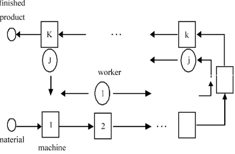
We consider a U-shaped production line with K ma-chines and J workers, which is shown in Figure 1. It is assumed that JK. There is enough raw material in front of machine 1. The material is processed at ma-chines 1 to K sequentially, and customers receives finished products from machine K. Workers deal with all machines in the same route and operate an item at each machine. Operation times at each machine may be different among workers, and the operation time of worker j at machine is denoted by k sj k, , which is deterministic. Worker starts his first operation at machine
j
j
k and visits machines
sequentially. The deterministic walking time from machine k to
1,
j j
k k 2,,K, 1, 2,
1
k
K
1 1 1, 2
k ,, is denoted by rk k, 1, where it is assumed that K
k i
. The
proc-essing time at machine is denoted by , which is deterministic. When a worker visits a machine, if the preceding worker is operating at the machine or the
[image:2.595.59.289.553.704.2]k
Figure 1. U-shaped production line
machine is processing the preceding item, then the worker must wait for the completion of operating or processing. The overall cycle time is defined as a time interval between successive outputs of finished products. We also define the cycle time of worker as the time interval between the successive arrivals of worker at machine . It is noted that the overall cycle time is the cycle time divided by the number of workers. The first cycle time of worker is the time interval between a start of first operation and the first arrival of worker
at machine . The th
j
j
1
j
j
1 n
n2
cycle time of worker is the time interval between the th and th arrivals for worker at machine 1.j
n1
nj
3. Cycle Time
3.1 Case of the Same Operation Times among Workers
In the case that operating times at each machine are the same among workers, from Nakade and Ohno (2003), when processing, operation and walking times are con-stant, the overall cycle timeCoverall is expressed as
, 1ˆ ˆ
1
max max , ,
overall
c k k k
k K
k K k K
C s i s
J
rk k
(1)where sk denotes the operation time at machine
and
k
ˆ 1,2, ,
K K . The overall cycle time is the great-est value of the maximal sum of the processing and op-eration times among machines and the time required for a worker to operate and walk around the production line without waiting for processing divided by the number of workers.
3.2 Case of Different Operation Times among Workers
We consider the case that operating times at each ma-chine may be different among workers. In this case, from Equation (1), the overall cycle time may be gue- ssed as
overall
C
, ˆ
1,2, ,
, , 1
1,2, , ˆ ˆ
1
max max ,
1
max .
overall
j k k
k K j J
j k k k
j J
k K k K
C s
J
s r
J
i
(2)
Ji , ˆ 1,2, ,
, , 1
1,2, , ˆ ˆ
max max ,
max .
j k k k K
j J
j k k k
j J
k K k K
C s s r
(3)From Equation (3), when processing times are zero, it is guessed that the cycle time is equal to the greatest value among times required for each worker to operate and walk around the line. However, under some specified cases, the cycle time is greater than this value, and the cycle time changes periodically. The examples are shown in the next section.
4. Periodicity of Cycle time
4.1 Numerical Examples
The set of operation times of each worker at each ma-chine is denoted by
1,1 1, ,1 , , , , , K l
J J K
s s S s s ,
where subscript is a number which distinguishes sets of operation times.
l
Let J3 and K4. It is assumed that processing times and walking times are zero, that is, ik 0 and for . Worker 1 starts his first operation at machine 1, worker 2 at machine 2 and worker 3 at machine 3. The first cycle is until the first arrival of a worker at machine 1. The th cycle is the
, 1
k k
r 0 kKˆ
[image:3.595.93.287.88.155.2]n
n2
Table 1. Cycle times for S 1
cycle\worker 1 2 3
1 8.0 7.0 6.0
2 8.0 8.0 8.0
3 8.0 8.0 8.0
4 8.0 8.0 8.0
5 8.0 8.0 8.0
6 8.0 8.0 8.0
Table 2. Cycle times for S2
cycle\worker 1 2 3
1 8.0 7.0 2.0
2 11.0 11.0 11.0
3 8.0 8.0 8.0
4 11.0 11.0 11.0
5 8.0 8.0 8.0
6 11.0 11.0 11.0
interval between
n1
th and th arrivals of a worker at machine 1.n
Cycle times, when operation times of each worker at
each machine are , are shown in Table 1.
Cycle times of all workers are 8 at all cycles except for the first cycle. This is the case that the cycle time does not change periodically. Then the cycle time 8 in Table 1 is equal to the value which is derived from Equation (3).
1 5,1,1,1 1, 5,1,1 1,1, 5,1 S
Cycle times, when operation times of each worker at
each machine are , are shown in Table 2.
In this case, the cycle time changes periodically. Except for the first cycle, cycle times of each worker take values of 8 and 11 alternately. The cycle time 8 in Table 2 is equal to the value which is derived from Equation (3). The cycle time 11 is more than the value which is de-rived from Equation (3).
2 5,1,1,1 1,1, 5,1 1, 5,1,1 S 4.2 Discussion
We investigate many examples including the above, and we have the following properties on the cycle time.
1) In many cases, in which the difference is not so large among workers, the cycle time is the same as Equa-tion (3).
2) If the cycle time changes periodically, then the pe-riod of the cycle time is two.
3) If the cycle time changes periodically, then the smaller cycle time is equal to the one which is derived from Equation (3), and the greater cycle time is more than the one which is derived from Equation (3).
4) Initial machines of each worker do not affect the cycle time if an order of arrivals of workers at machine 1 does not change, where, for example, the orders “4,3,2,1” and “2,1,4,3” are regarded as the same order.
5) An order of arrivals of workers at machine 1 affects the cycle time.
The movements of each worker when operation times are equal to are shown in Figure 2. When operation times are equal to , for example, worker 2 tends to wait for the completion of operation of worker 3 at ma-chine 2 since mama-chine 2 is bottleneck for worker 3. And also, since machine 3 is bottleneck for worker 2, worker 2 operates at his bottleneck machine (machine 3) after the waiting at machine 2. This makes the cycle time of worker 2 amplified. If a worker has his bottleneck ma-chine after the bottleneck mama-chine of his preceding worker, then the cycle time of the worker is amplified. In the next cycle, worker 3 finished his operation at his bot-tleneck machine (machine 2) while worker 2 operates at
2
S
2
[image:3.595.73.272.501.724.2]Periodicity of Cycle Time in a U-Shaped Production Line with Heterogeneous Workers under Carousel Allocation 268
Figure 2. Movements of workers
1 4 3 2 1 4 3 2
5 0 1 1 5 0 1
1
1
2
3
4
1 5
1
1
1 0
0
0 1
5
1 5
1
1 1
1
1
[image:4.595.58.265.292.603.2]Worker
Figure 3. Arrow diagram for S1
1 4 3 2 1 4 3 2
5 0 1 1 5 0 1
1
1
2
3
4
1 5
1
1
1 0
0
0 1
1 1
1
1
1
Machine
5 1 5
Worker
Figure 4. Arrow diagram for S2
his bottleneck machine (machine 3) and the succeeding machines (machines 4 and 1). Therefore in this cycle worker 3 does not need to wait for the completion of the operation of worker 3 at machine 2. Hence the cycle time of worker 2 does not increase in this cycle. These are why the cycle time of worker 2 changes periodically in Figure 2.
On the other hand, when operation times are equal to , machine 3 is bottleneck for worker 3, machine 2 for worker 2 and machine 1 for worker 1. When worker 3 operates at machine 3, worker 2 tends to operate at ma-chine 2, and when worker 2 operates at mama-chine 2, worker 1 tends to operate at machine 1. That is, when a certain worker operates at his bottleneck machine, the other workers tend to operate at their bottleneck ma-chines. Therefore, cycle times are the same value in every cycle.
1
S
Let us change initial machines of each worker under the condition that the order of arrivals of workers at ma-chine 1 does not change. Worker 1 starts his first opera-tion at machine 1, worker 2 machine 3 and worker 3 machine 4. Operation times of each worker at each ma-chine is equal to . Then cycle times of each worker are equal to the results which are shown in Table 2. In all examples which we investigate, initial machines of each worker do not affect cycle times.
2
S
Compare sets of operation times with . The set is the case that operation times of workers 2 and 3 at each machine are exchanged in the set . From results of Table 1 and 2, the order of arrivals of workers at ma-chine 1 affects the cycle time.
1
S S2
2
S
1
S
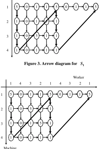
Figures 3 and 4 are arrow diagrams which show cycle times of worker 1 for successive two cycles. Numbers on vertical axis denote machines and numbers on horizontal axis denote workers. Nodes denote operations of each worker at each machine and numbers on nodes denote operation times of each worker at each machine. Figure 3 shows the case of and Figure 4 shows the case of . Worker 4 is a dummy worker and the operation times are zero. When we follow arrows from the most upper left node, which is referred as to the initial node, to the most upper right node, which is referred as to the last node, if the sum of cycle times on the route is maximal, then the sum is equal to the sum of cycle times of worker 1 for successive two cycles. In Figure 3, on the route that the sum of cycle times is maximal, the sum of cycle times is 16. This value is equal to the sum of cycle times for successive two cycles in Table 1. Similarly, in Figure 4 the sum is 19. This value is equals to the sum of cycle times for successive two cycles in Table 2. With Com-paring Figures 3 with 4, in Figure 3 there are two nodes at which the operation time is equal to 5 on all routes, while in Figure 4 there are two nodes on which the op-eration time is equal to 5 on some routes, and there are three nodes on which the operation time is equal to 5 on others.
1
S
2
S
5. Conclusions
[image:4.595.59.259.441.610.2]car-ousel allocation. In the case that operation times at each machine are different among workers, we investigate the cycle time. Under some specific cases, the cycle time changes periodically. We have some insights into the periodicity of the cycle time and discuss cycle times. For future research the condition that the cycle time changes periodically is derived.
REFERENCES
[1] Y. Monden, “Toyota production system,” An integrated Approach, 3rd edition, Engineering and Management
Press, Georgia, 1998.
[2] G. J. Miltenburg, “One-piece flow manufacturing on u-shaped production lines: A tutorial,” IIE Transactions, Vol. 33, pp. 303–321, 2001.
[3] K. Nakade and K. Ohno, “Separate and carousel type allocations of workers in a U-shaped production line,” European Journal of Operational Research, Vol. 145, pp. 403–424, 2003.