Essays on volatility forecasting

Dimos S. Kambouroudis

A Thesis Submitted for the Degree of PhD at the

University of St. Andrews

2012

Full metadata for this item is available in Research@StAndrews:FullText

at:

http://research-repository.st-andrews.ac.uk/

Please use this identifier to cite or link to this item: http://hdl.handle.net/10023/3191

This item is protected by original copyright

Essays on Volatility Forecasting

Dimos S Kambouroudis

This thesis is submitted for the degree of PhD

at the

University of St Andrews

1. Candidate's declarations

I, Dimos S Kambouroudis, hereby certify that this thesis, which is approximately 56000 words in length, has been written by me, that it is the record of work carried out by me and that it has not been submitted in any previous application for a higher degree.

I was admitted as a research student in September 2006 and as a candidate for the degree of PhD in September 2006; the higher study for which this is a record was carried out in the University of St Andrews between 2006 and 2011.

Date Signature of candidate

2. Supervisor's declarations

I, hereby certify that the candidate has fulfilled the conditions of the Resolution and Regulations appropriate for the degree of PhD in the University of St Andrews and that the candidate is qualified to submit this thesis in application for that degree.

Date Signature of supervisor

3. Permission for electronic publication

In submitting this thesis to the University of St Andrews I understand that I am giving permission for it to be made available for use in accordance with the regulations of the University Library for the time being in force, subject to any copyright vested in the work not being affected thereby. I also understand that the title and the abstract will be published, and that a copy of the work may be made and supplied to any bona fide library or research worker, that my thesis will be electronically accessible for personal or research use unless exempt by award of an embargo as requested below, and that the library has the right to migrate my thesis into new electronic forms as required to ensure continued access to the thesis. I have obtained any third-party copyright permissions that may be required in order to allow such access and migration, or have requested the appropriate embargo below.

The following is an agreed request by candidate and supervisor regarding the electronic publication of this thesis:

Access to printed copy and electronic publication of thesis through the University of St Andrews.

Date

Essays on Volatility Forecasting

Dimos S Kambouroudis

This thesis is submitted for the degree of PhD

at the

University of St Andrews

Stock market volatility has been an important subject in the finance literature for

which now an enormous body of research exists. Volatility modelling and forecasting

have been in the epicentre of this line of research and although more than a few

models have been proposed and key parameters on improving volatility forecasts have

been considered, finance research has still to reach a consensus on this topic. This

thesis enters the ongoing debate by carrying out empirical investigations by

comparing models from the current pool of models as well as exploring and proposing

the use of further key parameters in improving the accuracy of volatility modelling

and forecasting. The importance of accurately forecasting volatility is paramount for

the functioning of the economy and everyone involved in finance activities. For

governments, the banking system, institutional and individual investors, researchers

and academics, knowledge, understanding and the ability to forecast and proxy

volatility accurately is a determining factor for making sound economic decisions.

Four are the main contributions of this thesis. First, the findings of a volatility

forecasting model comparison reveal that the GARCH genre of models are superior

compared to the more ‘simple’ models and models preferred by practitioners. Second,

with the use of backward recursion forecasts we identify the appropriate in-sample

length for producing accurate volatility forecasts, a parameter considered for the first

time in the finance literature. Third, further model comparisons are conducted within

a Value-at-Risk setting between the RiskMetrics model preferred by practitioners, and

the more complex GARCH type models, arriving to the conclusion that GARCH type

models are dominant. Finally, two further parameters, the Volatility Index (VIX) and

Trading Volume, are considered and their contribution is assessed in the modelling

and forecasting process of a selection of GARCH type models. We discover that

This thesis is the product of hard work, dedication and many sacrifices and would

have not been completed without the help and support of certain individuals. In the

next few lines I would like to take the opportunity to thank the people who have stood

by me during this journey.

I would first like to thank my supervisor Professor David McMillan for his limitless

help, support and patience. David made available his support in a number of ways, not

only as a supervisor but as a mentor and friend. A simple thank you would not be

enough to express my gratitude to you.

I am most grateful to my parents to whom I owe my deepest gratitude. Thank you for

always being there for me, thank you for inspiring me, making me appreciate the

value of education and thank you for showing me the way…

“Now father, you cannot tell me to study any more…”

Last but not least I would like to thank my wife Melisa and my daughters Ioanna and

Marina. Thank you for your patience, for putting up with me during this process,

supporting me through the highs and lows, for keeping me sane and for adding value

List of contents

1. INTRODUCTION ... 10

2. LITERATURE REVIEW ... 19

2.1INTRODUCTION... 19

2.2MODELLING VOLATILITY... 25

2.2.1 Early applications for volatility measurement ... 25

2.2.2 Simple Models ... 28

2.3STOCHASTIC VOLATILITY (SV) ... 33

2.4IMPLIED VOLATILITY (IV) ... 35

2.5EMPIRICAL REGULARITIES OF ASSET RETURNS... 36

2.6ARCH/GARCHMODELLING... 42

2.7TIME VARYING GARCH ... 48

2.8STATE OF THE LITERATURE... 50

3. A VOLATILITY FORECASTING EXERCISE ... 59

‘SIMPLE’ VERSUS GARCH TYPE MODES & EMERGING VERSUS DEVELOPED ECONOMIES ... 59

3.1INTRODUCTION... 60

3.2VOLATILITY IN EMERGING MARKETS... 63

3.3DATA AND METHODOLOGY... 66

3.3.1 Data ... 66

3.3.2 Methodology ... 69

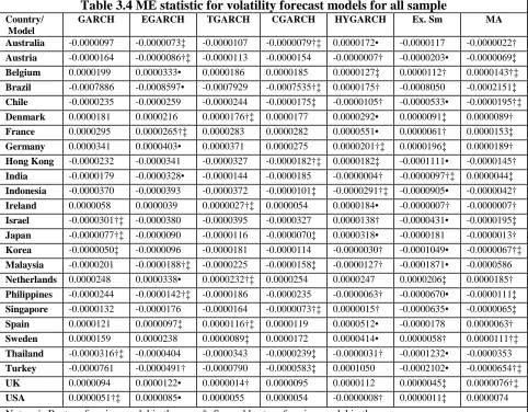
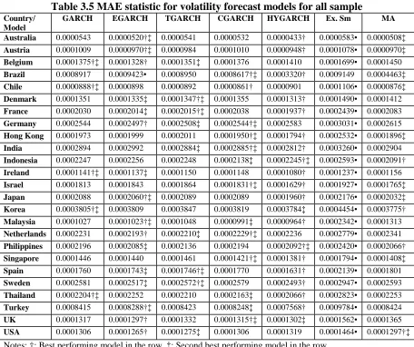
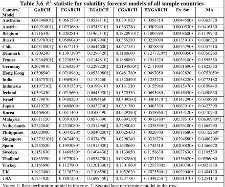
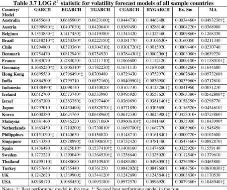
3.4EMPIRICAL RESULTS AND ANALYSIS... 79

3.5FURTHER CATEGORISATION OF RESULTS (DEVELOPED VS EMERGING) ... 89

3.6CONCLUSION... 97

4. A BACKWARD RECURSION VOLATILITY FORECASTING EXERCISE ... 102

4.1INTRODUCTION... 103

4.2DATA AND METHODOLOGY... 105

4.2.1 Data ... 105

4.2.2 Methodology ... 105

4.3RESULTS AND ANALYSIS... 108

4.3.1 GARCH(1,1)... 109

4.3.2 EGARCH... 113

4.3.3 TGARCH ... 116

4.3.4 CGARCH... 120

4.3.5 Moving Average ... 123

4.4CONCLUSION... 127

5. A VALUE-AT-RISK VOLATILITY FORECASTING EXERCISE... 131

5.1INTRODUCTION... 131

5.2RISK MANAGEMENT IN FINANCE AND VAR ... 133

5.3DATA AND METHODOLOGY... 138

5.3.1 Data ... 138

5.3.2 Methodology ... 140

5.4RESULTS AND ANALYSIS... 148

5.5SUMMARY AND CONCLUSION... 166

6. A VOLATILITY FORECASTING EXERCISE WITH VIX AND VOLUME ... 169

6.1INTRODUCTION... 169

6.2VOLATILITY INDEX VIX ... 172

6.3VOLUME (VO AND VA)... 176

6.5EMPIRICAL RESULTS... 186

6.6FURTHER ANALYSIS:A FORECAST ENCOMPASSING EXERCISE... 192

6.7CONCLUSION... 202

7. SUMMARY AND CONCLUSIONS ... 204

7.1SUMMARY... 204

7.2CONCLUSIONS... 209

8. BIBLIOGRAPHY AND REFERENCES ... 214

1. Introduction

Stock market volatility has been an important subject in the finance literature for

which now an enormous body of research exists, especially after the 1987 stock

market crash. Volatility modelling and forecasting have been in the epicentre of this

line of research and although more than a few models have been proposed and key

parameters on improving volatility forecasts have been considered, finance research

has still to reach a consensus on this matter. With this thesis we wish to enter the

ongoing debate and conduct research by comparing models from the current pool of

models as well as explore and propose further key parameters to be considered in

improving the accuracy of volatility modelling and forecasting.

Accurately modelling and forecasting volatility is of significant importance for

anyone involved in the financial markets. In general, according to Figlewski (2004),

the term volatility is associated with risk, and high volatility is thought of as a

symptom of market disruption implying that assets and securities are not fairly priced.

For example increased volatility will have important implications for investors.

Investors may have to alter their investment strategies either by shifting their

investment portfolios towards less risky short-term assets, or they could use

immunisation strategies for their portfolios. On the other hand policymakers are also

affected by increased volatility and would pursue regulatory reforms either by trying

to reduce volatility directly or by assisting financial markets and institutions to adapt

On the other hand other activities such as risk management, portfolio management

and selection, derivative pricing and hedging are examples of activities that would

suffer without accurate volatility predictions. More specifically, Engle and Patton

(2001) mention: “A risk manager must know today the likelihood that his portfolio

will decline in the future. An option trader will want to know the volatility that can be

expected over the future of the life of the contract. To hedge this contract he will also

want to know how volatile is this forecast volatility. A portfolio manager may want to

sell a stock or a portfolio before it becomes more volatile. A market maker may want

to set the bid ask spread wider when the future is believed to be more volatile” p. 2.

As can be seen, the importance of accurately forecasting volatility is paramount for

the functioning of the economy and everyone involved in finance activities. In periods

of instability, volatility forecasting becomes even more important since governments,

the banking system, institutional and individual investors are trying to cope with

increased risk, increased volatility and lack of resources. Knowledge, understanding

and the ability to forecast and proxy volatility accurately could be a determining

factor for survival not only during turbulent times but also during periods of economic

growth, giving an advantage to whoever can successfully manage future volatility.

This is also the motivation of this thesis.

With this thesis we wish to add knowledge to the literature on volatility forecasting by

means of empirical investigation and propose the use of a number of key parameters

that should be considered in the modelling process of volatility forecasting. There are

four main contributions of this thesis. First, after performing a volatility exercise it is

and models used by practitioners. Second, for the first time in the finance literature

the question of identifying appropriate in-sample lengths for out-of-sample forecasts

is raised. The answer to this question is proven to support the views raised by

practitioners, that large in-sample periods are not necessary for producing accurate

volatility forecasts. Third, within a Value-at-Risk volatility forecasting setting the

RiskMetrics model, which is preferred by practitioners for its simplicity, does a

poorer job compared to the more complex GARCH type models. Fourth, the

contribution of the Volatility Index (VIX) and Trading Volume on the forecast ability

of a selection of GARCH type models cannot be ignored since a better level of

accuracy is achieved; however GARCH type forecasts are dominant.

Apart from the main contributions mentioned above other issues are also examined.

The sample selection, with the exception of the last empirical chapter where due to

data availability only a small number of countries are considered, consists of large

number of countries with a good mix of both developed and emerging economies in

order to identify any trends, patterns or other regularities. Furthermore, the nature of

the topic allowed for comparisons of methods between those used mainly in academia

and methods preferred by finance practitioners.

The structure of the thesis comprises of a literature review chapter, four empirical

chapters and a conclusion chapter. The next chapter (Chapter 2) is the literature

review chapter. Definitions of stock market volatility are given and its importance for

the finance literature highlighted. The main focus of this chapter is on the exploration

of the different models used for forecasting volatility, looking first at the ‘simple’

volatility clustering, the leverage effect and stationarity then the more advanced

GARCH type models are introduced. The models introduced in this chapter are used

in the rest of the thesis. Then follows a section on the state of the literature setting the

scene for the research questions we address in this thesis.

In Chapter 3 a straightforward comparison exercise of volatility models is performed.

This type of exercise has been a popular theme within the finance literature with often

conflicting results. Stock market volatility has been the subject of numerous studies in

the finance literature -see literature review chapter for more details, particularly after

the stock market crash of 1987. Similarly, modelling and forecasting volatility became

a popular area of research within finance, for academics and practitioners alike.

Taking part in this debate a comparison between representative models from the two

popular model categories, the ‘simple’ models; namely the Exponential Smoothing

and the Moving Averages and the more ‘advanced’ GARCH type models capturing

the features of volatility clustering, the leverage effect and volatility persistence,

which are found to exist in the data.

In an attempt to identify any possible global trends the sample is selected from a wide

geographical perspective (Europe, Asia, America and Australia) including developed

and emerging markets, since the majority of the empirical work has been carried out

mainly on developed markets. For all the countries of the sample daily closing prices

of the countries representative index spanning over two decades are obtained. Four

measures of comparison are used in this exercise and a further dimension is explored

based on the classification of the sample markets in order to identify the existence or

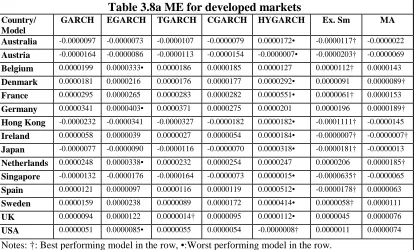
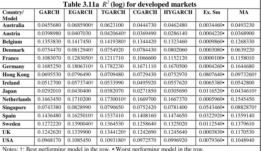
that the more advanced GARCH type models do a better job overall than the ‘simple’

models. More specifically in the order of the asymmetric models first followed by the

long memory models and finally in third place the ‘simpler’ time series models. When

the country classification is taken into account a clearer picture emerges in the ranking

of the results for the developed economies than for the developing economies,

however for both the developed and emerging economies there is no contest in

identifying the worst performing model as the exponential smoothing model.

Chapter 4 takes a look at a key parameter ignored so far by academic research within

the volatility forecasting literature, and that is specifying the ideal size of the

in-sample period required for producing accurate forecasts. The question of ‘how much

previous data do we need in order to produce accurate forecasts?’ This question

introduces the notion of recursive forecasts for the first time within volatility

forecasting where the debate is between practitioner/investors and

researchers/academics who share different views regarding this question.

Respectively, a small in-sample period (small number of observations) is preferred to

a large in-sample period (large number of observations) when forecasting volatility

due to cost and storage restrictions.

The same dataset from Chapter 3 is used and a good selection of the better performing

models from the same chapter are selected, more specifically from the GARCH genre;

GARCH(1,1), EGARCH, TGARCH and CGARCH and the representative ‘simple’

model Moving Average. The main objective of this exercise is to determine the

optimal number of in-sample observations to produce the most accurate forecasts. For

fixed end date to the start of the variable in-sample period producing a forecast for

every window of 60 observations. For each forecast (window) the forecast

comparison measure of Mincer-Zarnowitz (MZ) performed, regressing the true

volatility value on the produced forecast value obtaining the coefficient of

determination for comparison purposes.

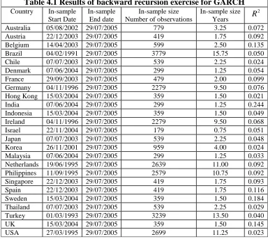
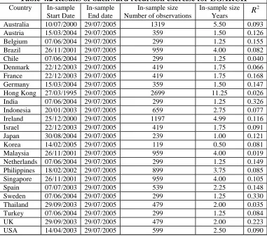
The results show a degree of homogeneity. For most countries of the sample and for

the majority of the models large in-sample periods are not necessary for producing the

most accurate forecasts supporting the practitioners/investors view; however the

models that produce the most accurate forecasts require larger in-sample durations.

Furthermore, when taking into account the country classification smaller in-sample

durations are required for producing accurate forecasts in emerging markets but more

accurate forecasts produced for countries in developed economies.

The superiority of the GARCH genre of models has been highlighted by the finance

literature (see Chapters 2 & 3), however, the aim of Chapter 5 is to seek an answer to

the question whether the in-sample superiority of the GARCH model carries over to

out-of-sample forecasting, or whether forecasts from the RiskMetrics model known

for its simplicity of application and is preferred by the finance professionals can

provide adequate forecasts of volatility in a Value-at-Risk setting.

In the academic finance literature the problems associated with the RiskMetrics model

have been reported, more specifically with respect to the undefined unconditional

variance and the model’s inability to produce long-horizon forecasts. On the other

literature, which not only does not suffer from the same problems the RiskMetrics

approach does but also is better able to capture the inherent time-dependency within

volatility.

Using a large selection of thirty-one international stock markets including those of the

G7, thirteen further European markets and eleven further Asian markets RiskMetrics

forecasts were compared to those of the GARCH type models within a VaR

framework. The following conclusions are reached. When forecasting the 1% VaR the

RiskMetrics model does a poor job and is typically the worst performing model, on

the other hand the GARCH type models and more specifically the APARCH model is

preferred. However when forecasting at the 5% VaR then the RiskMetrics model

performs adequately. In short, the RiskMetrics model only performs well in

forecasting the volatility of small emerging markets and for broader VaR measures.

This chapter and aspects from chapter 3 were published1 in the International Review of Financial Analysis, a copy can be found in the appendix of the thesis.

In the final empirical chapter (Chapter 6) we assess the effect of the Volatility Index

(VIX) and Trading Volume on volatility forecasting. Both VIX and Volume have

appealing and useful properties, which the finance literature has recognised, resulting

in both these factors to be considered in forecasting exercises mainly individually, and

with only a very small number of recent studies assessing the impact of both VIX and

Volume together within the context of volatility forecasting.

1 _{Reference: McMillan, D. G., and Kambouroudis, D., (2009), “Are RiskMetrics forecasts good}

VIX has proven to be a useful instrument for forecasting volatility, since it is a

forward looking measure and is defined as a benchmark of expected short-term

market volatility upon which futures and options contracts on volatility can be written.

On the other hand Trading Volume is caused by information flow which is positively

correlated to price changes suggesting that a relationship between Trading Volume

and volatility also exists.

Following on from the previous empirical chapters VIX and Volume data are used

within a GARCH type model framework and the testing procedure of

Mincer-Zarnowitz (MZ) is used followed by forecast encompassing tests in order to establish

whether there is added value in incorporating the two parameters within the

forecasting process. Three main markets selected are the UK, France and the USA

mainly due to data availability. The results suggest that both VIX and Volume

improve on the informational content of the GARCH type models, VIX does a better

job in this process than Volume, but better results are reported when VIX and Volume

are used together. In answering the question whether VIX produces better forecasts

than the GARCH genre of models, the answer is no but the informational content of

VIX cannot be ignored.

Finally, Chapter 7 summarises the main findings: the superiority of the GARCH

genre of models in volatility forecasting exercises over the ‘simpler’ time series

models, models preferred by finance practitioners and VIX; and that the in-sample

duration is an important determinant for out-of-sample forecasts. This chapter also

provides concluding remarks as well as propositions for future research on the issues

Note: The use of the first person plural ‘we’ instead of the first person singular ‘I’ is

used throughout the thesis. Any work published from this thesis will be co authored

2. Literature review

2.1 Introduction

Stock market volatility has been the subject of many studies over the past few

decades. The main impetus for this interest began after the 1987 stock market crash

where, for example, the Standard & Poor’s (S&P) composite portfolio dropped from

282.70 to 224.84 (20.4 %) and the Dow-Jones Average fell by 508 points in one day.2 The term stock market volatility refers to the characteristic of the stock market to rise

or fall sharply in price within a short-term period (from day to day or week to week).

A complete definition of volatility in the economic sense is given by Andersen et al.

(2005) in a more recent working paper: “Volatility within economics is used slightly

more formally to describe without a specific implied metric, the variability of the

random variable (unforeseen) component of a time series. More precisely, in financial

econometrics, volatility is often defined as the (instantaneous) standard deviation (or

σ “sigma”) of the random Wiener-driven component in a continuous-time diffusion

model. Expressions such as “implied volatility” from option prices rely on this

terminology” (p.1). This phenomenon is not new since throughout the post-war

period, stock markets, commodity markets, bond markets and foreign exchange

markets have recorded sharp movements.

In a review essay by Cochrane (1991) several issues are being addressed: “what,

ultimately, is behind day-to-day movements in prices? Can we trace the source of

movements back in a logical manner to fundamental shocks affecting the economy…?

Are price movements due to changes in opinion or psychology, that is, changes in

confidence, speculative enthusiasm…?” (p. 463). Furthermore economists and other

academics were concerned about the efficient market hypothesis and volatility; do

volatility tests reject the efficiency itself? As Shiller (1989) and Cochrane (1991)

mention, volatility tests do not prove that markets are inefficient. “Volatility tests are

in fact only tests of specific discount-rate models, and they are equivalent to

conventional return-forecasting tests… Thus, the bottom line of volatility tests is not

‘markets are inefficient’ since ‘prices are too volatile’, but simply ‘current

discount-rate models leave a residual’ since (discounted) returns are forecastable”, Cochrane

(1991), p. 464.

The determinants of financial market volatility, according to Shiller (1988) are

difficult to define, simply because economists and other researchers do not have a

proven theory of financial fluctuations. Theories that exist are often unconvincing.

One explanation of financial market volatility, given by Shiller (1988), is market

psychology. Investors appear sometimes to react to each other instead to some

fundamental event, and this process can set into motion large market swings. He

proved with his survey that market psychology was a key factor behind the stock

market crash of 1987, suggesting that on the day of the crash investors were not

responding to any specific news item but to news of the crash itself. Mishkin (1988)

agreed with Shiller that stock market volatility is difficult to explain, and although he

did not fully agree with his survey evidence, he too believed that factors other than

underlying economic fundamentals may have played a role in the stock market crash

The notion of speculation has been mentioned and was related to the ‘bad’ effects of

volatility.3 There is a debate about speculators and their impact on volatility, suggesting that increased volatility is undesirable and reductions in volatility are

desirable. This is misleading as it fails to recognise the link between information and

volatility, Antoniou and Holmes (1995). Within the Efficient Market Hypothesis

(EMH) literature there is a positive relationship, with a rapid reaction between the

arrival of information and price fluctuations. Consequently, if the flow of information

increases, in an efficient market, price movements will be more frequent (more

volatile), Antoniou et al. (1997).

Generally, increased volatility has been viewed as an undesirable consequence of

destabilising market forces such as speculative activity, noise trading or feedback

trading. Increased volatility could come as a result of an innovation, by reflecting the

actual variability of information regarding fundamental values. So increased volatility

may not necessarily be undesirable, Bollerslev et al. (1992).

Ross (1989) using a simple model under the condition for no arbitrage, proved that

the variance of price change will be equal to the rate (or variance) of information

flow. “In an arbitrage-free economy, the volatility of prices is directly related to the

rate of flow of information to the market. In a simple model the two were found to be

identical. This result links volatility tests to efficient market hypothesis which specify

the information set the market uses for pricing” (p. 17). By this we can conclude that

the volatility of the asset price and in consequence the volatility of the market as a

whole, will increase as the rate of information increases. In the opposite case arbitrage

opportunities will exist.

Mishkin (1988) also addressed the role of monetary policy in the face of financial

market volatility. Monetary policymakers have two alternatives when dealing with

volatility. They can attempt to reduce the volatility by intervening in markets, or they

can stay out of the markets but stand ready to function as lender of last resort in the

event of a financial crisis. He indicated a preference for the latter.

A stock market fall could be harmful for the economy. It has been observed,

according to Becketti and Sellon (1991), that stock volatility has an effect on the

economy through consumer spending, business investment spending and also could

disrupt the smooth functioning of the financial system by leading to structural

regulatory changes.

First, stock price volatility hinders the performance of the economy via consumer

spending. Immediately after the October 1987 drop in stock prices, economic

forecasts predicted sharply weaker economic growth. It was believed that the fall in

stock prices would reduce consumer spending, because of the weakening of consumer

confidence and wealth. Second, investors may perceive a rise in the stock market

volatility as an increase in the risk of equity investments. Thus, investors could shift

their funds to less risky assets i.e. bonds, although long-term investments contain an

element of risk too. This reaction would tend to raise the cost of equity for firms

issuing stock and to misallocation of resources Antoniou et al. (1997). Small and new

purchase of stock in large and well-known firms. Finally, extreme stock price

movements could also have an effect on the financial mechanism and lead to

structural changes. Systems working under normal price volatility may be unable to

cope with extreme price changes. The system itself may contribute to volatility if

investors are unable to complete stock transactions. Changes in market rules or

regulations may be necessary to increase the resilience of the market in the face of

greater volatility, Becketti and Sellon (1991).

Changes in volatility have important implications for investors and policymakers.

Investors may have to alter their investment strategies. They would have two

alternatives in order to cope with increased volatility. They could either shift their

investment portfolios towards less risky short-term assets, or they could use

immunisation, for example hedging or other strategies, for their portfolios. For

instance, investors after the October 1987 crash tried to adjust to volatility by

restructuring their portfolios. This explains the sharp drop in stock purchases after the

crash. Individual investors reduced their direct purchases of stocks and also shifted

away from stock mutual funds. As a consequence, retail stock brokerages and mutual

funds have experienced reduced profitability and have scaled back operations and

employment.

On the other hand policymakers may pursue regulatory reforms by either trying to

reduce volatility directly or by assisting financial markets and institutions to adapt to

increased volatility. In practice policymakers have focused on the latter, improving

the ability of financial markets and institutions to weather increased volatility. For

institutions and market makers, policymakers have encouraged greater capitalisation.

Increased capital allows these institutions to weather greater financial volatility

without incurring the liquidity and solvency problems that might disrupt the

functioning of financial markets, Becketti and Sellon (1991).

The topic of volatility is of significant importance to anyone involved in the financial

markets. In general volatility has been associated with risk, and high volatility is

thought of as a symptom of market disruption, with securities unfairly priced and the

malfunctioning of the market as whole. Especially within the derivative security

market volatility and volatility forecasting is vital as managing the exposure of

investment portfolios is crucial, Figlewski (2004). More recently the literature has

focused on the ability to forecast volatility of asset returns. There are many reasons

why forecasting volatility is important according to Walsh, Yu-Gen Tsou (1998), for

example, option pricing has traditionally suffered without accurate volatility forecasts.

Controlling for estimation error in portfolios constructed to minimise ex ante risk,

with accurate forecasts we have the ability to take advantage of the correlation

structure between assets. Finally when building and understanding asset pricing

models we must take into account the nature of volatility and its ability to be

forecasted, since risk preferences will be based on market assessment of volatility.

It is apparent that volatility is important, since it directly and indirectly affects the

financial system and the economy as a whole. The main aim of this chapter will be to

look into the aspects of volatility forecasting since in view of all the reasons explained

above researchers, policymakers and investors will have an advantage when

insight into volatility forecasting will be given but first it is necessary to explore the

different models used when estimating volatility.

2.2 Modelling Volatility

The complex issue of measuring and quantifying volatility is still one of the main

challenges academics and practitioners are dealing with. Over the years several

models and methods have been proposed but still we are far from any generally

accepted formula. In the next section some of the earlier applications and models of

volatility measurement are described.

2.2.1 Early applications for volatility measurement

In order to quantify and model volatility we first must define volatility. In his work,

Figlewski (2004), does a good job in setting the groundwork for understanding the

concept of volatility using finance basics. Starting from the ‘efficient markets’ or

‘random walk’ model, asset price movements can be described by an equation like:

(2.1)

where; and

He mentions, “the return at time t, r , is the percentage change in the asset price S, _t

future

ε

ε

characteristic of efficient market pricing: past price movements give no information

about the sign of the random component of return in period t, Figlewski (2004), p. 3.

Modern option pricing theory began in 1973 with Black and Scholes (1973), where

volatility plays a central role in determining the fair value for an option or a derivative

instrument with option features. The input parameters required in order to produce a

Black–Scholes option price are: the current stock price, the option strike price, the

risk free interest rate, the option’s remaining time to maturity and the future volatility

of the underlying asset. All parameters except the latter one can be obtained easily by

the market Figlewski (2004).

(2.2)

Options and futures benefit from price fluctuations of the underlying asset as well as

of securing a portfolio against price losses or hedging a planned purchase against a

possible price increase Maris et al. (2004). In deriving the option pricing formula,

Black and Scholes needed to model stock price movements over very short time

intervals in order to adjust their trading strategy after continually rebalancing a

portfolio consisting of an option and its underlying stock. The formula they adopted

(equation 2.2) is a logical extension of the random walk model over time. This is a

limiting random walk process as the time interval goes to zero, keeping the mean and

the variance of returns per year constant. The result is a lognormal diffusion model

where the dS is the asset price change over time (infinitesimal time) interval dt,µ is

with mean of zero and variance of one at dt, and

σ

deviation of the annual return, Figlewski (2004).

In order for empirical research to analyse and draw conclusions, an array of models

for measuring volatility were developed. Volatility modelling and forecasting has

been the subject of vast empirical and theoretical research over the past decades as

volatility has become one of the most important concepts in the finance literature.

Often volatility is measured by the standard deviation or variance of returns as a

simple risk measure. Other models such as Value at Risk (VaR) modelling, for

measuring market risk, and the previously mentioned Black and Scholes model, for

pricing options, require the estimation of volatility. We consider the returns process

given by:

t t

t m

r = +ε (2.3)

where mt is the conditional mean process (which could include autoregressive (AR)

and moving average (MA) terms), where the error term can be decomposed as εt = σt

zt with zt an idiosyncratic zero-mean and constant variance noise term, and σt is the

volatility process to be estimated and forecast, with forecast values denoted ht2. The

sample data is split between the in-sample period, t=1,…,T, and the out-of-sample

period t=T,…,τ. In order to generate a historical ‘actual volatility’ series on the basis

of which volatility forecasts may be generated using the statistical models described

below, the methodology by Pagan and Schwert (1990) is followed in representing past

2.2.2 Simple Models

The term ‘simple’ for the models described below refers to the traditional and widely

used in the past techniques not only in finance but other disciplines too. The list of

models belonging in this category is extensive and only few models will be described

here.

Random Walk

If volatility fluctuates randomly the optimal forecast of next period’s volatility is

simply current actual volatility:

2 2

1 t

t

h₊ =σ (2.4)

This random walk model thus suggests that the optimal forecast of volatility is for no

change since the last observed value.

Historical Average

Extrapolation of the historical mean of the volatility process is perhaps the most

obvious means of forecasting future volatility. Furthermore, if the distribution of

volatility has a constant mean all variation in estimated volatility could be attributed

to measurement error and the historical mean computed below gives an optimal

forecast for all future periods:

∑

− =

= +

τ

σ τ 1

2 2

1

1

t t

t

T

Simple Moving Averages

Under the moving average method volatility is forecast by an unweighted average of

previously observed volatilities over a particular historical time interval of fixed

length:

∑

+ = P

j j

t

p h

1 2 2

1

1 _σ

(2.6)

where P is the moving average period or ‘rolling window’. The choice of this interval

is arbitrary.

Exponential Smoothing

Under exponential smoothing the one-step ahead volatility forecast is a weighted

function of the immediately preceding volatility forecast and actual volatility:

2 2

2

1 t (1 ) t

t h

h₊ =φ + −φ σ (2.7)

where φ is a smoothing parameter constrained to lie between zero and one, such that

for φ=0, the exponential smoothing model reduces to a random walk model, while for

φ=1 weight is given only to the prior period forecast. The value of φ is determined

empirically by that value which minimises the in-sample sum of squared prediction

errors. Empirical studies have also confirmed the usefulness of the exponential

In 1989 JP Morgan developed the RiskMetrics approach to volatility using the simple

exponential smoothing model described above in order to quantify and assess the risk

exposure of the firm. This approach received wide acceptance in the finance world as

well as in academia when in 1992 JP Morgan launched the RiskMetrics methodology.

Since its inception several versions of the RiskMetrics Technical Document have

been published, in addition the establishment of the Value at Risk framework also

triggered the popularity of the RiskMetrics approach. Empirical studies have also

confirmed the usefulness.

Exponentially Weighted Moving Average (EWMA)

The exponentially weighted moving average model is similar to the exponential

smoothing model discussed above, but past observed volatility is replaced with a

moving average forecast, as in the simple moving average model:

2 2 2

1 ₁

1

(1 ) P

t t _j j

h h

p

φ φ σ

+ = + −

∑

Exponentially weighted moving average models (EWMA) are an extension of the

historical volatility measure allowing more recent observations having a stronger

influence on volatility forecasting than older observations. When applying the

EWMA modelling the latest observation carries the largest weight and weights

associated with previous observations decline exponentially over time. In contrast to

the simple historical volatility model, volatility is affected more by recent events

which carry more weight than events further in the past and the effect of a single

Smooth Transition Exponential Smoothing method4

These models allow parameters to change over time in order to adapt to changes in

the characteristics of the time series. Taylor (2004) proposes the use of logistic

function of a user –specified variable adaptive smoothing parameter. Within the

volatility forecasting modelling framework this would be formulated as:

(2.9)

where; .

The smoothing parameter varies between zero and one, and adapts to changes in the

transition variable and where and are used as transition variables in the

similar way the sign and size of past shocks have been used as transition variables in

non-linear GARCH models, Taylor (2001). In the words of Granger and Poon (2003)

the smooth transition model is a more flexible version of the exponential smoothing

model where the weight depends on the size and sign of the previous return. This

approach is analogous to the GARCH type models for allowing the dynamics of the

conditional variance to be influenced by the ‘leverage effect’ and the ‘volatility

persistence’, characteristics found in stock market data and discussed in more depth in

section 2.3.

Other volatility models

Due to the popularity of the topic volatility modelling forecasting several other

models have been proposed, this list is also extensive and for this reason only a small

mentioned that a simple measure of volatility is the standard deviation of returns of an

index. Becketti and Sellon (1991) measure volatility by the annual standard deviation

of monthly returns in the S&P 500 Composite Stock Price Index. This is a measure of

dispersion of monthly returns about the average return for each year. Another method

to measure normal volatility mentioned from the same source (Becketti and Sellon,

1991) is by using the interquartile range, the distance between 25th and 75th percentile of the monthly returns within a year.5

In a more recent review paper Poon and Granger (2003) attempt to make a distinction

between the standard deviation, volatility and risk. Standard deviation,

σ

2

σ , is computed from a set of observations as:

2 2

1

1

ˆ ( )

1 N

t t

R R N

σ

=

= −

−

∑

where R is the mean return. The argument here is that the standard deviation is only

the correct dispersion measure for the normal dispersion measure for the normal

distribution. The link between volatility and risk is a questionable one. Risk is usually

associated with small or negative returns, whereas most measures of dispersion make

no distinction. The two examples mentioned by Poon and Granger (2003), are: first is

the Sharpe ratio, defined as the return in excess of risk free rate divided by the

standard deviation which is frequently used as an investment performance measure

occasionally penalizes occasional high returns. Second the ‘semi-variance’, a concept

developed by Harry Markowitz (1991), where only the squared returns below the

mean are used, but this method is not easy to apply and it is not widely used.

Grabel (1995) uses two general models the Keynesian Volatility Index and the

Neo-Classical Volatility Index (type 1, 2). These indices derive from the theory behind

each approach, which are respectively: “…that assets yield some normal return over

time based on their underlying fundamental value. The magnitude of the deviation

from the asset’s fundamentals-based return constitutes asset volatility” and “volatility

in the Keynesian case is simply given by the magnitude of asset return fluctuations”

(p. 906, Grabel, 1995).

2.3 Stochastic Volatility (SV)

Stochastic Volatility (SV) models have their roots in mathematical finance and

financial econometrics. Interest in this class of models dates at least to the work of

Clark (1973) where as suggested modelling asset returns as a function of a random

process of information arrival. This so-called time deformation approach yielded a

time-varying volatility model of asset returns (Chysels, Harvey and Renault, 1996).

Tauchen and Pitts (1991) noted that if the information flows are autocorrelated, then a

stochastic volatility model with time varying and autocorrelated conditional variance

might be appropriate for price-change series, linking information arrival to asset

returns. A different view was expressed by Hull and White (1987) and Melino and

Turnbull (1990) where stochastic volatility models could also arise as discrete

approximations to various diffusion processes of interest. For example as mentioned

in Chysels et al. (1996), they were not directly concerned linking asset returns to

models for the underlying asset. Taylor (1986) on the other hand formulated a discrete

time series SV model as an alternative to ARCH models instead of using a

likelihood-based approach but the Method of Moments (MM) in order to avoid integration

problems associated with evaluating the likelihood directly. As mentioned in Granger

and Poon (2005) the volatility noise term makes the SV model a lot more flexible, but

as a result the SV model has no closed form hence making Maximum Likelihood

unsuitable. In addition to the MM approach other estimation approaches were

proposed such an example would be the Quasi-maximum likelihood (QML) estimator

of Harvey et al (1994) nevertheless if volatility proxies are non-Gaussian this method

is also inefficient. Other alternatives are variations of the Generalised Method of

Moments (GMM) approach through simulations, analytical solutions, and the

likelihood approach through numerical integration6. The Stochastic Volatility model is defined as:

t i t

R =µ +ε (2.11)

whereεt=ζtexp(0.5ht) and ht=ω+βht-1+υt.

Note:

υ

2.4 Implied Volatility (IV)

As previously mentioned in section 2.2.1, the Black-Scholes option pricing formula

states that the option price is a function of the price of the underlying asset, the strike

price, the risk free interest rate, the time to option maturity and the volatility of the

underlying asset. Given that the above parameters are observable, once the market has

produced a price for the option, volatility could be derived using backward induction,

and then use the volatility measure (value) that the market used as input. This measure

of volatility is called option implied volatility. Option implied volatility is often

interpreted as a market’s expectation of volatility over the option’s maturity. Because

each asset can have only one volatility measure, difficulties arise when options with

similar maturities but different strikes produce different implied volatility estimates

for the same asset, Granger and Poon (2005). Some examples of earlier studies where

the basic Black-Scholes option pricing model was used are Latane and Rendleman

(1976), Chiras and Manaster (1978) and Beckers (1981). More studies also examined

implied volatility as a source of information, for examples studies by Day and Lewis

(1990) who conclude that time-series models of conditional volatility outperforms

implied volatility, and Lamoureux and Lastrapes (1993) who find that information

contained in historical volatility is superior to that contained in implied volatility.

Furthermore Canina and Figlewski (1993) also find that implied volatility has no

correlation with future volatility and hence “to measure the “market’s” volatility

estimate (we) must not just take the implied volatility” (pp. 678).

On the other hand a good number of studies can be found in the finance literature

Hansen (2002). More recently, Christensen, Hansen and Prabhala (2001), Blair, Poon

and Taylor (2001), Ederinton and Guan (2002), Pong et al. (2004) and Jiang and Tian

(2005) take longer data sets, high frequency data and account for structural changes

concluding that implied volatility is a more efficient forecast for future volatility than

historical volatility.

In the most recent literature review paper by Granger and Poon (2005), it is concluded

that the predictive ability of implied volatility cannot be ignored nor underestimated

compared to other volatility models. More specifically “implied volatility appears to

have superior forecasting capability, outperforming many historical price volatility

models and matching the performance of forecasts generated from time series models

that use a large amount of high frequency data” (pp. 489-490). The importance of

implied volatility is highlighted in Chapter 6.

2.5 Empirical regularities of asset returns

Following the seminal work of Mandelbrot (1963) and Fama (1965), many

researchers have reported that the empirical distribution of stock returns is

significantly non-normal. In particular, the kurtosis of the stock returns time series

appears to be larger than the kurtosis of the normal distribution (the time series of

stock returns are leptokurtic), the distribution of stock returns can be skewed either to

the right (positive skewness) or to the left (negative skewness), and the variance of the

stock returns may not be constant over time and indeed volatility exhibits clustering.

Researchers regarded this as the persistency of the stock market volatility and the

financial analyst called this uncertainty or risk. Volatility measured by the variance

and covariance and was accepted for decades Chong et al. (1999). In order to select an

appropriate volatility model, we must have a good idea of what empirical regularities

the model should capture. Some of the important regularities for asset returns are

presented below (Bollerslev et al. 1994).

Thick tails

Asset returns tend to be leptokurtic. According to the literature on the modelling of

stock returns, stock returns have thick-tailed distributions and are modelled as

independent and identically distributed (iid). This empirical regularity has been

documented by Mandelbrot (1963), Fama (1963, 1965), Clark (1973), and Blattberg

and Gonedes (1974).

Volatility Clustering

Volatility clustering where ‘large changes tend to be followed by large changes of

either sign, and small changes tend to be followed by small changes’ as Mandelbrot

(1963) wrote, is a visible phenomenon when asset returns are plotted through time.

A Sample Financial Asset Returns Time Series

-0.08 -0.06 -0.04 -0.02 0.00 0.02 0.04 0.06

1/01/90 11/01/93 9/01/97

Return

Date

Figure 2.1 Source: Brooks (2008)

Leverage effects

The ‘leverage effect’ noted by Black (1976), refers to the negative correlation

between stock prices and changes in stock volatility. Fixed costs such as financial and

operating leverage provide a partial explanation for this phenomenon. A firm with

debt and outstanding equity usually becomes more highly leveraged when the value of

the firm falls. This raises equity returns volatility if the returns on the firm as a whole

are constant. However, as argued by Black (1976), the response of stock volatility to

the direction of returns is too large to be explained by leverage alone; Christie (1982)

and Schwert (1989).

Non-trading periods

Information that accumulates when financial markets are closed is reflected when the

markets reopen. For example, information accumulating at a constant rate over time,

then the variance of returns over a period from the Friday close to the Monday close

Fama (1965) and French and Roll (1986), information accumulates at a slower rate

when markets are closed than when they are open. Variances are higher after

weekends and holidays but not as high as if the rate of information was constant.

French and Roll (1986) for example have found that volatility is 70 times higher per

hour on average when the market is open than when it is closed, and similar results

found by Baillie and Bollerslev (1989) on foreign exchange rates.

Forecastable events

Forecastable releases of important information are associated with high ex ante

volatility. For example, Cornell (1978), Patell and Wolfson (1979, 1981) show that

individual firms’ stock returns volatility is high around earnings announcements, and

Harvey and Huang (1991, 1992) find that fixed income and foreign exchange

volatility is higher during periods of heavy trading by central banks or when

macroeconomic announcements are made. There are also intraday predictable changes

in volatility. Several papers have found that volatility is much higher at the opening

and closing of a trading day for stocks and foreign exchange; Harris (1986), Gerity

and Mulherin (1992) and Baillie and Bollerslev (1991). One explanation for high

volatility at the open is the accumulated information, as mentioned above, but the

high volatility at closing is more difficult to explain.

Volatility and serial correlation

Both LeBaron (1992) and Kim (1989) find a strong inverse relationship between

volatility and serial correlation for the U.S. stock indices and for the foreign exchange

respectively. The above finding appears to be remarkably robust to the choice of

Co-movements in volatilities

Black (1976), mentions that in general when volatilities change, they all tend to

change in the same direction. Several studies8 support this argument of the existence of common factors explaining volatility movements in stock and exchange rates.

Engle et al. (1990) show that US bond volatility changes are closely linked across

maturities. The commonality of volatility changes holds not only across assets within

a market, but also across different markets. For example, it was found by Schwert

(1989) that U.S. stock and bond volatilities move together and Engle and Susmel

(1993) and Hamao et al. (1990) have discovered links between volatility changes

across international stock markets.9

As Bollerslev et al. (1994) mention, the fact that volatilities move together should be

encouraging to model builders, since it indicates that a few common factors may

explain much of the temporal variation in the conditional variances and covariances of

asset returns, which is the basis of the ARCH modelling.

Macroeconomic variables and volatility

Stock values are considered to be related and closely tied to the health of the

economy, so it is natural to expect that measures of economic uncertainty such as

conditional variances of industrial production, interest rates, and money growth,

should help explain changes in stock market volatility Bollerslev et al. (1994).

Schwert (1989), finds that although stock volatility rises sharply during recessions and

financial crises and drops during expansions, the relation between macroeconomic

8

Diebold and Nerlove (1989) and Harvey et al. (1992). 9

uncertainty and stock volatility is surprisingly weak. On the other hand Glosten et al.

(1993), uncover a strong positive relationship between stock return volatility and

interest rates.

Long memory

Stock market returns contain little serial correlation, Fama (1970) and Taylor (1986),

which complies with the Efficient Market Hypothesis. However, according to Ding et

al. (1993), this empirical fact does not suggest that returns are independently

identically distributed. More specifically they find that: “… not only there is

substantially more correlation between absolute returns than returns themselves, but

the power transformation of the absolute return also has quite high autocorrelation

for long lags” (p. 83). It can be argued that the ‘long memory’ feature appears to be

present for which models capturing volatility need to account for.

Up and until the beginning of the 1980’s the above data regularities were not

addressed by the more traditional and simple time series and other models developed

in order to model and forecast volatility. However based on the above mentioned

problems, in 1982 Engle proposed and developed the Autoregressive Conditional

Heteroscedasticity model, the ARCH model, a new methodological approach which

received wide acceptance in the finance literature. This is the main topic of the next

2.6 ARCH/GARCH Modelling

This section describes a selection of the most popular in the finance literature models

belonging to the ARCH/GARCH genre.

ARCH

Most papers refer to the test of Autoregressive Conditional Heteroscedasticity

(ARCH) model. This was developed by Engle (1982), in his attempt to test for the

ARCH effects on the variance of the United Kingdom inflation, and latter reviewed

by Engle and Bollerslev (1986). This model accounts for the difference between the

unconditional and the conditional variance of a stochastic process. While

conventional econometric models operate under the assumption of a constant

variance, the ARCH process allows the conditional variance to vary over time,

leaving the unconditional variance constant. To model for ARCH effects in the

conditional variance of a random error, ε_t we have:

2

1

( )

t t t

h =Var

ε

where h2_t is the conditional volatility and Ω_t−1 is the information set.

The ARCH (q) specification is given by:

h2 2

1 a

t i t i

i

a

ω ε₋

=

GARCH (Generalised ARCH)

The GARCH model of Engle (1982) and Bolerslev (1986) requires joint estimation of

the conditional mean model and the variance process. On the assumption that the

conditional mean stochastic error, εt, is normally distributed with zero mean and

time-varying conditional variance, ht2, the GARCH (1,1) model is given by:

2 2 2

1 t t

t h

h₊ =ω+αε +β (2.14)

where all the parameters must be positive, while the sum of α + β quantifies the

persistence of shocks to volatility. The GARCH (1,1) model generates

one-step-ahead forecasts of volatility as a weighted average of the constant long-run or average

variance, ω, the previous forecast variance, ht2, and previous volatility reflecting

squared ‘news’ about the return, εt2. In particular, as volatility forecasts are increased

following a large return of either sign, the GARCH specification captures the

well-known volatility clustering effect. The GARCH models are also capable of capturing

leptokurtosis, skewness (besides volatility clustering), which are the features most

often observed in empirical analysis.

EGARCH (nonsymmetrical dependencies)

Depending on the nature of the data the researchers are investigating, several

variations of the above models are used. For example, a more appropriate technique

that incorporates asymmetries in the modelling of volatility is the Exponential

GARCH or EGARCH model introduced by Nelson (1991). This approach captures

illustrated by Appiah-Kusi and Pescetto (1998) when examining the spillover effect of

the “Tequila effect” on African countries. The EGARCH model of Nelson (1991)

provides an alternative asymmetric model:

) log( )

log( 2_{1 t}2

t t

t t

t h

h h

h₊ =

ω

α

ε

γ

ε

β

where the coefficient γ captures the asymmetric impact of news with negative shocks

having a greater impact than positive shocks of equal magnitude if γ<0, while the

volatility clustering effect is captured by a significant α. Finally, the use of the

logarithm form allows the parameters to be negative without the conditional variance

becoming negative.

TGARCH (Threshold-GARCH, non-symmetrical dependencies)

The GARCH model, although non-linear in the conditional mean error postulates a

linear dependence of conditional variance upon squared past errors and past variances,

such that opposite shocks of equal magnitude inevitably incur the same effect upon

variance. A significant issue that has arisen in the empirical application of GARCH

models to financial data, and equity market data in particular, concerns the potential

for an asymmetric effect of positive and negative shocks upon conditional variance.

As noted by Black (1976), and expanded upon further by Christie (1982), a negative

relationship often holds between current variance and the sign of past shocks. Thus, a

negative shock increases the conditional variance by a greater amount than an equal

consider one of the most popular asymmetric-GARCH models, namely the

threshold-GARCH (Tthreshold-GARCH) model of Glosten, Jagannathan and Runkle (1993):

2 2

2 2

1 t t t t

t I h

h₊ =ω+αε +γε +β (2.16)

where the leverage effect is captured by the dummy variable It, such that It =1 if ε

t-1<0, and It=0 if εt-1>0. Thus, in the TGARCH (1,1) model, positive news has an

impact of α, and negative news has an impact of α+γ, with negative (positive) news

having a greater effect on volatility if γ > 0 (γ < 0).

APARCH (Asymmetric Power ARCH)

An alternative model capturing the information asymmetry developed by Ding et al.

(1993) is the asymmetric power-ARCH, APARCH model, where the power parameter

on the standard deviation is estimated and not imposed:

δ δ

δ

_ω

_α

_ε

_γε

_β

1 1 1 1

1( − − − ) + −

+

= t t t

t h

h (2.17)

Where δ>0 and γ captures any asymmetric effect of positive and negative news upon

volatility.

QGARCH (Quadratic GARCH)

A model that copes with skewed returns in a similar way to the GJR model is the

Quadratic GARCH model proposed by Engle and Nq (1993) and further developed by