Physiological Responses to Roller Coaster Rides: A Pilot Study on the Differences between Virtual Reality and Real World Measures

(1)

A Pilot Study on the Differences between Virtual Reality and Real World Measures

Luise Warnke University of Twente

Master Thesis

Author Note

Date: August 26, 2019

(2)

Abstract

Introduction: The aim of the study was to measure and analyse arousal of roller coaster passengers in both VR and real-world to make a comparison between these situations. To make arousal testable two approachesare introduced: separating the ride in contiguous

phases vs. grouping data by roller coaster elements.

Study 1: Participants watched roller coasters in virtual reality while their EDA and HR was measured. A decrease of these measures from the first to the last phase was found.

Only a weak association of roller coaster elements with specific arousal reactions was ob-served.

Study 2: With a small group of participants an amusement park was visited to ride real-world roller coasters. No phase-dependent change of arousal was found. However, some roller coaster elements were accompanied with specific changes in arousal. For all roller coasters continuous EDA and HR is reported.

Conclusion: Even though no direct comparison between VR and real-world was con-ducted our research implies that both conditions have different effects on real-time arousal. We conclude that VR roller coasters can not be seen as an equivalent alternative to

(3)

Introduction

Those familiar with the Misattribution of Arousal Theory might have come across this classic example: someone steps on a roller coaster and after getting off again strangers seem much more attractive (Meston & Frohlich, 2003). But roller coasters have much

more capacity for psychological research than that. They have the special feature of making the rider undergo physical strain comparable to car racing, space shuttle take-offs or aerobatic flight manoeuvres (“Orders of Magnitude (Acceleration)”, n.d.). At

the same time riders of roller coasters do not undergo the cognitive burden of keeping control over their vehicle, maintaining an overview of flight data or calculating good flight paths. Roller coasters therefore yield good preconditions to quantify emotional and

force-induced arousal which influences the limit for mental workload of those working in high-force environments (Koglbauer, Kallus, Braunstingl, & Boucsein, 2011).

Despite this advantage of roller coasters for studying force-induced changes in psy-chophysiology little research has been conducted on them so far. And, of the existing research, many studies have been based on virtual reality (VR). Since results from VR

have been reported as if they were true for real roller coasters the question arises whether roller coasters in VR actually have the same impact as riding one in the real world. To an-swer this question, a two-part study was conducted with the aim of comparing responses

between these two situations. For the first study VR was employed, the second part was then conducted in an amusement park.

For our studies we measured reactions as arousal following being exposed to specific

(6)

mea-sure arousal we employed variables relating to heart rate (HR) and electrodermal activity (EDA). In general, changes in HR can point to both parasympathetic as well as sym-pathetic nervous system activity (Ernst, 2017) and happen within a short time frame

after exposure to the arousing stimulus (4-8 seconds; Baumgarten, Baldrighi, Vogel, & Thümler, 1980; Globisch, Hamm, Esteves, & Öhman, 1999). Besides HR, cardiovascular activity can also be expressed as measurements of heart rate variability (HRV). While

HR is the (local) average of or current expected number of heart beats per minute, HRV expresses how much the temporal distance of single heart beats varies (for a review of HRV see Shaffer, McCraty, & Zerr, 2014). EDA is the collective term changes in skin

conductance which occur when sweat glands are filled with sweat (Dawson, Schell, & Filion, 2016). A difference can be made between skin conductance level (SCL), the tonic component of EDA, and skin conductance response (SCR), the phasic responses of EDA

(Braithwaite, Watson, Jones, & Rowe, 2015). Responses of EDA are approximated to happen three seconds after the event.

What are the physiological effects of roller coaster rides?

To know whether effects of real roller coasters differ from those in VR we first need to know which psychophysiological effects have been reported before. And even though most research on physiological reactions to roller coaster rides has come from the field

of medicine, some relevant information about psychological effects can be inferred from their findings.

The most common way of describing effects in the papers discussed here is by

(7)

which phase arousal is the highest.

One option is that most arousal is perceived before the ride. For example, Rietveld and van Beest (2007) reported an increase of dyspnea, i.e. stress-related difficulty or

inability to breath, for persons suffering from asthma before roller coaster rides with dyspnea comparable to baseline after the roller coaster ride. Interestingly, they also found that participants’ HR did not increase immediately before the ride. The opposite,

a spontaneous increase of HR and SCR, has been found by several other scholars (Hinkle, 2016; Kuschyk, Haghi, Borggrefe, Wolpert, & Brade, 2007; Pieles et al., 2017). One special case is a study by Baumgartner, Valko, Esslen, and Jäncke (2006) for which an increase

of SCR amplitude sums was reported but no such effect for HR. Since the mentioned change in psychophysiological signals happens when the roller coaster moves up the lift hill, where no strong g-forces act on the riders, Kuschyk et al. (2007) argue that the response must be emotional. This theory can be confirmed by a study on water slides. Most of the participants reached their highest HR while waiting for their turn at the top of the stairs, thus without externally caused motion (Hokanson, Brauer, Hokanson,

Eldridge, & Maginot, 2016). In the study at hand we should also see an increase of arousal before the ride. To allow a quantitative evaluation hereof we will follow the example of Baumgartner et al. (2006) and compare the average of the measurements on the lift hill

to those of the rest of the ride.

A second opinion, on where to find the most arousal during roller coaster rides, is that this is the case during the actual ride, thus, between the first drop and the end brake.

(8)

range of average HRmaxfrom 142 to 165 bpm, with a total average of 158 bpm. However, it should be mentioned that Pieles et al. (2017) measured heart rates of children at 13.3± 1.5 years of age. Since the only evidence against the maximum arousal falling in this time

frame is the study by Yamaguchi, Kanemaru, Kanemori, Mizuno, and Yoshida (2003) where, as mentioned above, arousal was not measured continuously, it is also likely that arousal is the highest during the actual ride. Note that this is mutually exclusive to the

above described lift hill effect.

This previous option is mutually exclusive to the third option: arousal is the high-est after a roller coaster ride. An increase of arousal from before to after the ride has

been reported in several studies for different physiological measures, for example for HR (Kuschyk et al., 2007; Pieles et al., 2017; Rietveld & van Beest, 2007) and blood pressure (Kuschyk et al., 2007; cf. Rietveld & van Beest, 2007 or SCR (Hinkle, 2016). However,

as Yamaguchi et al. (2003) noted this increase not necessarily has to be linear. In their study on responses of salivary α-amylase concentration to roller coaster rides they found a linear increase of arousal when participants were scared. On the other hand, when

par-ticipants reported to enjoy the ride a decrease of arousal during the ride and an increase above the initial level after the ride was found was found. Taking α-amylase as a marker for arousal, which like HR and SCR is directly influenced by sympathetic nervous system

activity, and considering that the salivary system has been found to react within short time (Maruyama et al., 2012), it could be concluded that effects during the ride are weak. However, to sample saliva during the ride Yamaguchi et al. (2003) placed test stripes in

(9)

Why are real world and VR roller coasters differently arousing?

Up to this point it was only discussed which part of roller coasters are considered to be arousing in earlier research. However, the goal of this study is to compare arousal between VR and the real world. Therefore the question arises why these two situations

are assumed to be different. To discuss this point factors to arousal are classified by a model proposed by Roscoe (1992). For his study on pilots flying complex manoeuvres he presumed that EDA and HR are objective measurements for workload. It is stated that

overall workload is a combination of cognitive, emotional and physical workload.

For the part of cognitive workload one of the main tasks of the rider is to main-tain a concept of one’s position in space. At least that is the conclusion of a study by

Baumgartner et al. (2006), who observed brain activity of person seeing VR roller coasters using LORETA and EEG. For those individuals increased activity was found over cortical areas associated with spatial presence, mental rotation and homeostatic functions during

the ride. These cognitive processes are supported by well-oriented head movements and free body motion (Wade & Jones, 1997). While the cognitive processes can be assumed to be present for both real and VR roller coasters, the auxiliary functions are limited during

real roller coaster rides. First, because passengers are restricted by safety belts around the hips or shoulders from freely moving their upper body, and second, because uneven tracks or quick changes in horizontal acceleration can make it difficult to stabilize one’s

head position. Therefore it can be hard for riders of real roller coasters to maintain a full concept of orientation and position in space, whereas riders of VR roller coasters who can move (almost) freely and are not affected by external forces, should have less trouble to

maintain spatial presence.

(10)

presence). Arousal of cortical areas associated with presence on the other hand has been found to increase arousal by (virtual) roller coasters (Beeli, Casutt, Baumgartner, & Jäncke, 2008). Especially in VR presence can easily be disturbed due to missing or

inconsistent sensory input. One extreme example hereof is the lack of wind during the ride. Even though this might not seem to be a major issue on it’s own, one needs to realize that often the only auditory input during on-ride videos of roller coaster rides is the sound

of the wind. But not only the feeling of wind is missing, likewise one lacks the feeling of the shown weather (e.g. when watching a video shot on a rainy day in a warm room) and the physical forces pushing one around in the seat. Besides multimodal discrepancies, VR

yields several lacks within modalities. For example VR glasses are restricted in the field of view they supply: while the shown image while looking straight is similar to human field of vision nothing can be seen when turning one’s eyes sidewards in VR. To shift one’s field

of view one has to turn the head towards the direction one wants to watch. Furthermore, it is often observed that VR glasses’ frame rate shortly drops after a head movement. Drops in frame rate again are related to loss of presence (Barfield & Hendrix, 1995),

and might therefore implicitly cause people to rather infer peripheral information than to turn their heads. While discrepancies like the ones named here could be a reason for loss of presence and therefore less affection by VR roller coasters, to our best knowledge

no research has been conducted on the relevance of complete sensory information in VR containing quickly changing environments.

Besides the anticipation factor discussed above both VR and real-world roller

(11)

result in a loss of presence in VR so individuals know they are safe (Owens & Beidel, 2015; Peperkorn, Diemer, & Mühlberger, 2015); other scholars however indicate that exposure to heights in VR has the same effect as in the real world (Emmelkamp, Bruynzeel, Drost,

& van der Mast, 2001). Emotional reception of roller coaster rides might additionally be tinted by the definitiveness of the decision to take the ride: when taking a virtual roller coaster ride one can quit at any time by taking off the glasses, whereas one has to take

the full ride when stepping on a roller coaster in the real world.

Opposite to what one might expect real roller coasters also have soothing factors to them. For one thing, on-ride videos used in VR often do not provide a preview of the

roller coaster to be taken, but start with the passenger sitting in the car. Consequently, riders in VR are not prepared for eventual loops or other elements on the ride. Real world passengers on the other hand get to see the roller coaster before they make a decision to

take it and have the time they stand in the queue to mentally prepare for the ride. For the other thing, real roller coasters are often taken in the presence of friends or at least a stranger that will respond to short glances to their side (Kissel, 1965). The presence of

another individual can have soothing effects when facing dangers. In VR on the contrary one is seated next to a stranger who will not respond to one gazing their way.

While no clear answer can be given to whether VR or real world is more arousing in

the realms of emotion and cognition, we can be sure that only real world roller coasters have an impact on physical state of the participant. That physical forces on roller coasters actually have an effect on participants physiology has been shown by Pieles et al. (2017).

(12)

virtual roller coasters are due to physical forces. However, it needs to be considered that the presence of physical forces has an impact on emotional and cognitive factors as well. For example, as stated above, shaking of the head caused by sidewards-directed forces

can inhibit one’s ability to stabilize gaze and therefore make it harder to orientate. Or physical forces pressing one in the seat or throwing one in the air might increase one’s feeling of presence and make possible risks more salient. Consequently, effects on arousal

seen in close temporal proximity to the impact of physical forces can not be considered mere results of these forces.

Judging from the evidence above the question what the difference between VR and

real-coasters is, might be answered with: During real roller coaster rides physical forces act on the passenger that elicit cognitive and emotional responses that are weaker in VR. What remains unclear is, how big the difference in response is. One way to answer to this

is by directly comparing arousal in VR with that in the real world. To do so, we measured psychophysiological data under both condition. Where forces are low, arousal should be mainly caused by emotional and cognitive processes and therefore data collected in VR

should closely resemble real-world data. Whereas, where forces are high, VR data should not be a good predictor for real-world data.

How can patterns in physiological arousal be quantified?

For analysing the real-time data a model was needed that can express the relation of several continuous variables (i.e. the physiological data) and discreet classes (i.e. the ele-ments of the roller coaster), and that can quantify the relation. For this purpose we used

(13)

psychophysiolog-ical data (Cho et al., 2017).

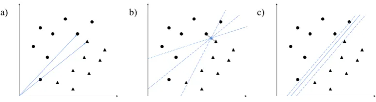
A SVM functions by finding the spatial separation between two classes when they are represented in a vector space. To find this separator, first, the vector to the data points

of both classes that are closest to each other is determined (i.e. the support vectors; see Figure 1a). The separator for the data is then set to run through the middle of the distance between the end points of the support vectors (Figure 1b). To find the best

separator, margins are set parallelly to both sides of the separation vector (Figure 1c). The better the fit, the more space between the margins and the less data between the margins or on the wrong side of the vector. A class is then defined as the space on one

side of the margin. Based on finding their position in the vector space and the previously defined classes the SVM can then make predictions for new data (Marsland, 2015).

Figure 1. Conceptual functioning of a SVM. a) Finding the support vectors: vectors are drawn from the origin of the vector space towards the two closest data points of each class. b) Possible separation vectors: All considered options for a separation vector run through the middle of the connection vector between the data points identified in a). c) Setting the margins: The wellness of a separation vector is determined by applying parallel lines to both sides through the closest data point on each side; the more distance to the margins the better the separation vector.

A SVM works with linear separators. Since not all data can be fit by linear sep-arators, predefined functions (i.e. kernels) can be used to transform data. Also, SVM can be modulated to compare more than two classes at once by comparing all available

[image:13.595.100.488.398.504.2]

(14)

In our study we can used a SVM to analyse how closely VR data resembles real world data. After checking whether for each data set on its own a prediction can be made, we used the VR data as a training set to define the classes. Then we let the trained

SVM classify the real-world data. Predictions for real-world data should be equally good when VR data is used for training as when real-world data is used for training, if they are not different. If, on the other hand, real-world effects are differing from those in VR

the SVM should perform better when trained on real-world data.

In summary, we want to answer whether psychophysiological effects of VR roller coasters are similar to those in the real world by determining the phase with the highest

arousal and by comparing the effect of single elements. We expect that arousal will either be the highest on the lift hill or during the actual ride. Additionally, we expect an increase of arousal from before to after the ride. In the direct comparison of arousal caused by

(15)

Study 1

For the first study participants watched VR simulations of roller coasters. The measured data was first analysed as to whether it confirmed observations made in earlier studies. Second, it was tested whether the data gathered could be used to classify itself. If in that

way internal predictability is proven data can be used as the training set for the second study.

Methods

Participants

Participants were recruited from the research pool of the University of Twente. The ethics committee of the Faculty of Behavioural, Management and Social Science at the University

of Twente granted approval. The request herefor is registered under the number 180062. Individuals self-reporting cybersickness1_{, motion sickness or vertigo during roller} coaster rides were strongly advised not to participate in the study. As it is the case

for real-world roller coasters persons with heart diseases or existing pregnancy were not admitted to undergo the stress of riding a roller coaster; however, since no strong physical forces were to be applied, back injury was not handled as an exclusion criterion. All

participants were compensated with 0.5 credit points which were necessary for course completion.

(16)

1.65). The female to male ratio was 11:3. For one participant no further data was col-lected because their physiological data could not be captured correctly and they therefore discontinued participation.

Materials

Informed consent. Informed consent was given on printed forms including a summary of the procedure and a reminder that participation is voluntary (see Appendix A).

A duplicate is given to the participant. In accordance with the General Data Protection Regulation (2016) consent is given in an active form (i.e. ticking “yes” or “no”) and participants are provided with information how data will be stored and distributed.

Demographics and experience questionnaire. A second paper form was used to assess participants’ demographics, their general tendency for motion sickness and ver-tigo, and how they perceived the VR (i.e. whether they felt sick and how scared and

happy they felt; see Appendix B). To avoid discomfort and to prevent reactivity partici-pants were offered to fold the paper twice after filling it in, so that the researcher will not immediately see the answers. However no participant used this option.

(17)

that were marked in each video can be found in Appendix C.

Table 1

Tags and criteria used for marking events in the videos of the roller coaster rides

Tag Description

Referential tags:

Start Start of the video. For reference only.

End End of the video. For reference only.

Ride events:

Brake The car starts hanging in the brakes at top ofBaron 1898’s lift hill. Corkscrew The car leaves the horizontal and starts ascending.

Drop Small drop before the lift hill. The car leaves the horizontal. End brake The car hits the end brakes. Marks end of the ride.

First drop The car starts moving down the descent after the lift hill. ForBaron 1898 this is the case when the brake is released, for the rest when the car leaves the horizontal.

Helix The car leaves the straight and leans into the curve.

Hop The highest point of a hop.

Immelmann see “Corkscrew”

Lift hill The car starts moving up the lift hill. Marks beginning of ride.

Loop see “Corkscrew”

Roll The car leans over or starts ascending into rolls.

Tunnel The car enters a tunnel.

VR simulation. Four VR simulations were presented to the participant using an Oculus Go headset. The main part of this headset is a box (size: 190 x 105 x 115 mm;

weight: 470 g) which contains a mobile device. Content is shown on a 5.5” display with a resolution of 2560 x 1440 px. To attach the device to the user’s head a strap is laid around the back of their head. Since the Oculus Go is a stand-alone device, a controller is

(18)

The VR videos shown were retrieved from YouTube (https://www.youtube.com/) and played in YouTube VR (Google LLC, 2018), an application devoted to playing content on VR glasses. Four VR videos were used in the study: three were on-ride videos of

roller coasters, the other was a neutral stimulus to keep the participant still but engaged during the basement measurement. Additionally, showing the video had the advantage that participants could get used to the VR and the control of the glasses, or report

cybersickness before being exposed to videos with high-motion content. The videos were arranged in playlists with the following order: (1) neutral video, (2) filler video (i.e. black screen; CandRfun, 2013), (3-5) roller coaster videos.

The neutral video shows four students guiding the viewer through the European Parliament in Strasbourg, France (Poolpio Immersive Content Agency, 2018). In about four minutes (03:57) participants get to see, among others, the plenary chamber, a short

interview with former President of the European Parliament Martin Schulz and the Par-liament’s press room.

Since SVM classifications were to be based on roller coaster elements a well-considered

selection of roller coasters had to be made. On the one hand, we wanted to include a broad range of elements. On the other hand, each element should preferably have several occurrences across all used roller coasters to create sufficient data for classification. An

additional limiting factor was that for the second study the same or similar roller coasters had to be available to grant comparability. Consequently, the choice of the used roller coaster videos was made in several rounds. First, the videos found when searching for

(19)

For example, roller coasters that are constructed to use a lot of space resulting in longer straight passages are rather uncommon in Europe and are therefore not considered (for example see Six Flag Magic Mountain’s The Riddler’s Revenge3). Another criterion was how prototypical the featured elements were, meaning that they did not include uncom-mon thrill elements like top hats or induction accelerated roller coasters. However, an exception was made for Efteling’s Baron 1898 (see below for more information); since it is

located in one of the parks considered for the second study it was not excluded. Finally, videos that on watching yielded a bad quality - even though they had a good upload qual-ity - were excluded. From the remaining videos three were chosen that together included

various thrill elements. This process resulted in the following choice of roller coasters:

• Mammut located at Tripsdrill (Cleebron, Germany): A wooden coaster with simple elements. After the first drop the car passes three helix-airtime hill combinations. The ride ends after five consecutive, alternating banked turns. The total ride from

entering the lift hill to the end brake lasts 143 seconds (02:23). The used video was uploaded by COASTERCREW Germany (2017). Due to the specific properties of wooden tracks the quality of the video is somewhat inferior to that of the other two

videos. However, only one participant indicated that this cause feelings of sickness and a few others felt that this decreased their enjoyment of the ride.

• Baron 1898 located at Efteling (Kaatsheuvel, Netherlands): A dive coaster with several inversions. After climbing the 40 meter lift hill the car is pushed to the edge

(20)

roll and a helix. Finally, the car drives over a bunny hop and though a banked turn. The ride from lift hill to end brake takes 54 seconds. The video uploaded by Efteling (2015) includes the waiting time of the car in the station. Matching the concept of

the ride (i.e. mining) a song is sung to the passenger by the “Witte Wieven” (i.e. Dutch mythological spirits) who threaten the miners to sabotage their work.

• Big Loop located at Hansa Park (Sierksdorf, Germany): A steel coaster with a high density of inversions. After leaving the station the car drives through a small drop to gain enough velocity to drive through a 180° curve and on the lift hill. Immediately after the first drop one passes two loops. These are followed by a banked turn into

two corkscrews. A helix leads the car back to the station. The ride from lift hill to end brake takes 99 seconds (01:39). The video used is uploaded by HeideParkResort (2017). Big Loopis a the same model as Efteling’sPythonwith a few minor changes.

Physiology sensor. Physiological data was measured using a Shimmer3 GSR sensor with a sampling rate of 256 Hz. Data from the sensors is collected through a

small box (6.5 cm x 3 cm x 1 cm), which was attached to the participant’s lower arm. From there data was transmitted via Bluetooth to a laptop where it was recorded. On the laptop Consensys (Shimmer, 2017) was used to display real time data and to tag the

start of the trials. Consensys automatically marks heart beats and derives heart rate and interbeat intervals. A full list of variables recorded for this study can be found in Appendix E.

Electrodermal activity (EDA) was measured with two electrodes attached to the palmar side of middle and ring fingers’ proximal phalanges on the non-dominant hand. Initially, photoplethysmogram (PPG) was collected from the outside of the index finger

(21)

to replaced for an ear clip due to material breakage. This resulted in a decrease of detected heart beats from on average 95.18 % of the recording for measurements from the participants’ fingers to on average 88.44 % for measurements from the earlobe.

Procedure

Participants were invited to one of the research cubicles at the University of Twente. After being asked whether they fall under any of the given restrictions and being informed about

the procedure and purpose of the study, participants had the possibility to ask questions. When they indicated to have understood the given information participants signed the informed consent.

Subsequently, the Shimmer electrodes were attached and the quality of the data was controlled on the laptop. Before participants put on the VR glasses, they were shown how to use the controller. This knowledge was immediately practised by starting the neutral

video. At the same moment as the participant started the video, the researcher started the recording of the transmitted data.

After the neutral video ended the participant was asked whether the glasses were

sitting comfortable without moving and whether they were free from cybersickness. If no such problems were reported the participant was asked to continue to the next video, the roller coasters. The moment that the participant pressed the controller’s trigger to

forward was marked by the researcher as the start of the video.

At the end of the last roller coaster the recording of physiological data was stopped and the participant could take off the VR glasses and the sensor. Then they were asked to

(22)

Data analysis

Data was analysed using Python 3.7. The code can be accessed at https://github .com/luisewarnke/rollercoaster; relevant samples are given in Appendix F. The workflow of the analysis is shown in Figure 2. As shown in Figure 2 analysis happened in three

phases which will be discussed in the following.

(23)

Preprocessing. Preprocessing is handled by the program’s data_prep.py script and its dependencies. For initial processing HR and EDA are treated separately.

HR and interbeat interval (IBI) were derived from PPG using the Python module

HeartPy (2018; van Gent, Farah, Nes, & van Arem, 2018). Heart rate was appended to the data frame for all samples between two heartbeats while IBI is only given with the corresponding heartbeat (see Appendix G, Sample 1).

EDA data is preprocessed using EDA-Explorer (Taylor & Jaques, 2016; Taylor et al., 2015). This package applies a low-pass filter to the data, identifies artefacts and SCR peaks. Specifically, we applied a sixth order Butterworth filter with a cut-off of 1 Hz.

For the artefact and peak detection scripts some changes were necessary, since they were written to be used with data sampled at 8 Hz (remember that our data was sampled at 256 Hz) and in accordance with Braithwaite et al. (2015) it was preferred to conserve the

high sampling rate for researching changes that were expected to happen in a short time frame. Which lines were changed specifically can be found in Appendix G.

Replication. In a second step the assumptions made based on earlier research

are tested. Herefor data is separated into five general segments: Baseline,Start to lift hill (S1),Lift Hill to first drop (S2),Ride form first drop to end brake (S3), and from the end brake to the End (S4). For each segment HRavg, average HRmax of 10 second intervals, SCL and number of SCR peaks per minute are calculated (see Appendix G, Sample 2). Paired two-sided t-tests were employed to test the three assumptions made from earlier research: S4 > S1, S2 > S1∪S3∪S4 and S3 > S1∪S2∪S4. Tests were called from

exploration.test_segments() using ttest_rel()from scipy.stats.

(24)

variables describing them. Therefore data is separated into snippets from 1.5 seconds before to 1.5 seconds after each tag. For each segment the variables given in Table 2 are calculated using the simplified code given in the table (code is taken from data_prep.

prepare_tags()). Note that all scores are relative. This is necessary for feeding them into the SVM: the algorithm thereof assigns weights to variables according to their absolute value; by rescaling variables to lay between 0 and 1 it is made sure that all variables will

be assigned the same weight.

Table 2

Variables used for classification and pseudocode used for their generation.

Variable Code Description

Cardiovascular activity: HRavg (data["HR"].mean()-baseline["HR_avg"]) /(220-baseline["HR_avg" ])

Average heart rate

HRmax

(data["HR"].max ()-baseline["HR_avg"]) /(220-baseline["HR_avg" ])

Maximum heart rate

HRmin-max

(data["HR"].max()-data ["HR"].min ())/(lim_HR-baseline["HR_avg"])

Difference between maximum and min-imum HR

NNavg

data.IBI.mean()/( snip_len*1000)

(25)

Variable Code Description SDNN

data.IBI.std()/(snip_len *1000)

Standard deviation of NN intervals

SDSD

[data.IBI[i]-data.IBI [i+1]].std()/(snip_len *1000)

Standard deviation of difference between successive NN intervals

RMSSD

[data.IBI[i]-data.IBI[ i+1]]**2.mean()**0.5/( snip_len*1000)

Root mean squared of standard deviation of difference between successive NN inter-vals

pNN20

len([data.IBI[i]-data. IBI[i+1]]>20)/len([data. IBI[i]-data.IBI[i+1]])

Proportion of successive differences larger than 20 ms out of all NN intervals

pNN50

len([data.IBI[i]-data. IBI[i+1]]>20)/len([data. IBI[i]-data.IBI[i+1]])

Proportion of successive differences larger than 20 ms out of all NN intervals

Electrodermal activity: SCRavg

EDA_peaks.mean()/data. EDA.max()

Average SCR

SCRn

(len(EDA_peaks)/snip_len )*60)

Number of SCR peaks per minute

Note. Adapted from Cho et al. (2017).

(26)

available (i.e. linear, polynomial, radial basis function (rbf) and sigmoid) the best fit was searched. To this end, the number of used variables and event tags was decreased iteratively, until the overall accuracy ( T P+T N

T P+T N+F P+F N, where T: True, F: False, P: Positive

and N: Negative) did not change considerably any more.

To identify variables that did not contribute to the classification the automatically assigned weights for each variable, which describe the used separation hyperplane, were

used. The magnitude of the vector corresponding to each variable tells how much it contributes (Bitwise, 2012). Variables that yielded a magnitude below 0.2 were excluded. The importance of the different events was analysed using the precision, recall (i.e. )

and F1-score (i.e. 2*_precisionprecision₊∗recall_recall). Theprecision tells the proportion of the data that was correctly classified as describing a certain event (i.e. True Positives (TP)) compared to all data that was classified to be describing this event, thus, also the data that actually not

describe the event (i.e. False Positives; _{T P}T P₊_{F P}). Therecall then describes the proportion of TP against data classified right, thus, TP and data that was correctly classified as not being the given event (i.e. False Negative; T P

T P+F N). The F1-score describes the

distribution of recall and precision. The better the SVM is able to classify the data the closer these three values get to 1. For decision of excluding elements from analysis the support (i.e. count of the event tag in test set) was used. Events of a support below 20

were excluded.

Design

The study used a within-subject time-series design. To prevent effects by stimulus order,

(27)

Results

Participant experience

Eight participants (19.51 %) reported to experience motion sickness and four (9.76 %) to experience vertigo in general. Cybersickness, vertigo or motion sickness during the VR session was reported by eleven participants (26.83 %); four of whom as well reporting

general motion sickness and three reporting general vertigo. In general the roller coasters made participants feel happy (much: 53.66 %; little: 43.90 %; not: 0 %), while ratings for scaredness were more diverse (much: 2.44 %; little: 46.34 %; not: 26.83 %; 24.39 %

did not fill in that question).

Heart Rate

First exploration of the HR data showed that presentation order had no noticeable influ-ence (see Figure H1). Strikingly, for almost half of the participants HR did not exceed

120 bpm. However, higher maximum HR was not associated with higher average base-line HR (see Figure H2). Additionally, when looking at the absolute maximum HR for each segement it was observed that the highest HR was reached during the baseline phase.

However no such effect can be observed when HRmaxper 10 seconds is used (see Figure 3). Regarding the expectations from earlier research the following was found. Neither for the full dataset (t(87) = -0.30; p = 0.76) nor for the separate videos (Mammut: t(27) = 1.10;p= 0.28;Baron 1898: t(28) = 0.88;p= 0.38;Big Loop: t(30) = -2.99; p= 0.006) was an increase of HR after the ride as compared to before the ride found. For Big Loop HR even seems to decrease.

(28)

Figure 3. Box plot of time-normalized maximum heart rate for each phase of the VR study.

other segments (t(90) = -2.93;p = 0.004;Mammut: t(29) = -2.52; p = 0.02;Baron 1898: t(29) = -2.25; p = 0.03;Big Loop: t(30) = -0.40; p = 0.69).

(29)

EDA

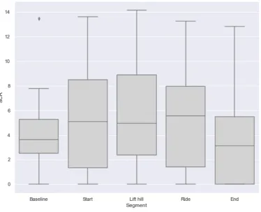
When looking at the number of SCR per minute a flooring effect becomes apparent Fig-ure 6. Though this effect is more pronounced for conditions one, four and five, scores for all conditions stretch towards zero Figure H4. Additionally, it can be observed that for

condition two the data measured during the baseline phase is lower than the rest of the session. Apart from that there seem to be no differences between the conditions.

Figure 4. Box plot of number of SCR per minute for each phase of the VR study.

[image:29.595.107.482.293.596.2]

(30)

-2.82; p = 0.008; Big Loop: t(30) = -2.60; p = 0.01).

Again, no sufficient support was found for the lift hill being the phase with most SCRs per minute (t(91) = -3.50; p < 0.001; Mammut: t(30) = -1.89; p = 0.07; Baron 1898: t(29) = -2.59;p = 0.01; Big Loop: t(30) = -1.59; p = 0.12). Nor for the ride being the most arousing part (t(91) = -7.20; p < 0.001; Mammut: t(30) = -4.03; p < 0.001; Baron 1898: t(29) = -2.93; p = 0.007; Big Loop: t(30) = -5.55; p < 0.001). That neither of the two moments has the highest score also becomes apparent when looking at the data split by participant (see Figure H5). No general trend can be observed; scores seem to be strongly individual.

Classification

The full linear model of all variables and event tags had an accuracy of 19.78 %. The same accuracy was found for the rbf and sigmoid kernel; for the polynomial kernel the accuracy

was 19.42 %. However, this difference vanished after the first iteration. Therefore for the remainder of this section the output of the linear kernel is discussed.

The tag which was best classified was Helix (precision = 0.20; recall = 1.00; F1 = 0.33). For all other tags the statistics returned zero. Therefore, decisions to remove tags from the model were in a first approach base on their representativeness of the sample (support is shown in Table 3).

(31)

Table 3

Total accuracy, vector magnitude for each variable and event tag support per iteration for data gathered during VR study.

Iteration 1 Iteration 2 Iteration 3

Accuracy 19.78 % 23.48 % 33.50 %

Variable

HRavg 2.7385 1.4297 1.2058

HRmax 2.4464 1.7328 1.6515

HRmin-max 2.6630 0.9215 0.8534

NNavg 1.5646 0.9601 0.6362

SDNN 0.6154 0.2807 0.3183

SDSD 0.5055 0.1982

RMSSD 0.0000

pNN20 3.5888 3.6466 1.3850

pNN50 2.5721 1.499 0.7026

SCRavg 5.5722 1.4993 1.8931

SCRn 0.1850

Event tag

Lift hill 28 27 24

First drop 27 34 33

Drop 20 22 23

Brake 9

Hop 51 42 38

Tunnel 22 19

Helix 55 58 69

Loop 18 19

Immelmann 13

Corkscrew 21 26 19

Roll 14

For the third iterationTunnelandLoopwere removed as well as SDSD. This resulted in an accuracy of 33.50 %, an increase by 10.02 %. Again the statistics forHelix increased (precision = 0.33; recall = 1.00; F1 = 0.50), but no clear classification could be made for the other tags.

The last iteration consisted of removing Corkscrew. Nevertheless, this decreased the model accuracy to 31.89 %. Consequently, the tag combination used for the third iteration seemed to be the one that was best to be classified.

(32)

parsi-monious variable combination is possible. For this HRmin-max, NNavg, SDNN and pNN50, which were yielding a magnitude below 1 were removed. This did not affect the prediction for the tag combination of iteration 3. Neither did it perform worse than a SVM using

all variables in classifying all tags.

Discussion

We tested three hypotheses derived from earlier research: first, that arousal is higher after a roller coaster ride than before it, second, that the lift hill is more arousing than the rest of the ride, and, third, that the phase between lift hill and end brake is more

arousing than the rest of the ride. In the study we carried out using VR neither could be confirmed. From data visualisation it rather seems that most participants are unaffected by the material. The decrease of SCR from the beginning of the session towards the end

might indicate that participants, after initial arousal from, for example, anticipation get more relaxed during the ride.

Initially the SVM showed a low accuracy which could only reach mediocre values

when removing rare events from the model. Changing the used kernel had no effect on the results. Data was classified with the same accuracy when only four variables were used for the model. Noticeably, the element that could be classified by the SVM is helices,

which are long curves. Indeed, many participants reported that they were most affected by curves with regards to dizziness and sickness, even if they were not affected by the rest of the ride (“I didn’t feel cybersickness as long as it was just going up and down.”). On

(33)

As noted above participants seemed to be highly aroused during the baseline phase. Even though this did not appear to be the case after time normalization the measured values were so high that we should discuss their possible origin here. One explanation

herefor is the, for most participants, unused experience of VR. After all, only one partic-ipant reported to regularly use VR glasses. However, no decrease of decrease of arousal from the first to the last roller coaster, which would indicate that participants are

get-ting used to the situation, was observed. An alternative explanation for the initial high arousal would be that, many participants experienced problems with the controller usage: instead of using the trigger to start the first video they pressed the “Back” button which is

located close to the button that was used to unlock the glasses (see Appendix D). When this occurred the participant came to see a pop-up window with a prompt to confirm that they want to leave the video player. At this point participants usually asked whether they

had to click “resume” whereupon they were informed that they confused the buttons and that they need to choose “resume” with the trigger. While most participants recovered from the mistake and now pressed the right button, others repeated the error and pressed

“Back” again. If the latter was the case the stress experienced by the participant could be observed externally in form of strong sweating, unrest (e.g. fidgeting on the chair) and emotionalized comments (e.g. “I think I am just too stupid for this.”). Participants were

calmed down (e.g. “You are not the first one who this happened to.”) and then step-by-step guided back to the right screen. Only in single cases was it necessary that the researcher had to take the glasses over and reset them to the right starting point. Whether

(34)

& Tremblay, 2012). Since no notes were taken on the occurrence of the above described error it was not possible to analyse data excluding the corresponding participants.

To avoid high stress by the way the VR glasses have to be controlled we want to

advise for future research to use remotely controlled VR glasses, so that the researcher can start and stop the videos. Additionally, a longer video could be used for the baseline measurement to give the participant more time to get used to the unused circumstances

(35)

Study 2

The goal of the second study was to collect data from participants on real roller coasters. To answer whether this data differs from that collected in VR, the data collected for the second study should ultimately be classified using the data collected for the first study as

the training set for the SVM.

Methods

Participants

Participants stemmed from a convenience sample, consisting of friends of the researcher. They actively declared interest in participation and content with not receiving a compen-sation. The following were handled as exclusion criteria: known heart disease, existing

pregnancy and history of back problems.

Seven individuals participated in the study; five male and two female. Age ranged from 21 to 27 (M = 23.43; SD = 2.37). No participant reported to suffer from motion sickness or fear of heights. Only one participant had been to the visited theme park before. Remarkably, one participant mentioned in conversation that they had not been on a roller coaster before.

Material

Informed consent. Again, informed consent was given on printed forms by ac-tive confirmation. The form was the same as for the first study besides slight changes to

the informative text (see Appendix I).

(36)

the question “Have you been at the Efteling before?” was added.

Roller coasters. The group visited the Dutch theme park Efteling. The roller coasters rode are described in the following:

• Bobbaan: A bobsled roller coaster. The ride starts by a small drop and a curve leading towards the lift hill. The first drop is followed by three alternating banked

turns. Then, while passing a hill, the car is braked slightly. This is again followed by three alternating curves and another brake on a hill. Finally, the car passes another curve, a helix and then two more curves. The total ride duration from lift hill to

end brake is 78 seconds.

• Joris en de Draak: A wooden coaster with two trains driving simultaneously to race each other. One train is called Vuur (Eng. fire), the otherWater. We rode on Water, therefore only that ride will be described. The ride starts with a flat helix as a first drop. After the actual drop the train drives over three hops on a ascending track. This is followed by another helix, several curves with hops and a last helix.

Seventy-five seconds (01:15) after the lift hill the car hits the end brakes whereupon the winner of the race is announced4_.

• De Vliegende Hollander: A water coaster which starts inside. The car is driving through a water-filled tunnel with several thrill elements: vases swinging over the passengers’ heads, driving through fog and pouring rain - a waterfall which splits to leave the passengers dry - and finally a big ship seemingly running the passengers’

(37)

laughter and see the Jolly Roger above their heads. This marks the end of the first section of the ride which takes about 150 seconds (02:30).

Now, the car is pulled up the lift hill and drops outdoors. The car drives over a hop and through a horseshoe. This is shortly followed by the splashdown. From the lift

hill to that moment the ride takes 41 seconds. This is the time frame considered for analysis. The remaining minute of the ride is the car driving through a lake back to the station. From leaving the station until the return there the ride takes 254

seconds (04:14).

• Baron 1898: See description above.

• Python: This roller coaster is nearly the same asBig Loop which is described above. The main difference is that before the drop into the double loop the car drives

through a 180°curve. The ride lasts 78 seconds (01:18).

• Vogel Rok: An enclosed roller coaster which is, except short small-scale light effects, kept in the dark. The ride comprises a few helices and takes approximately 58

seconds.

Tagging scheme. The same tags as for Study 1 were used with one minor change

for theEnd brake tag which forDe Vliegende Hollander equals the splashdown. The tem-poral position of the tags was derived from the motion data collected with the Shimmer3

sensor (see Data Analysis).

Physiology sensor. EDA and PPG were measured using Empatica E4 wrist-bands. On the wristband the necessary sensors are build in a little box (25 g; 4.4 cm x

(38)

but also to tag times. As long as the device is turned on, data is collected and stored in the internal memory. To read the internal memory the program E4 manager (Empatica, 2018) is used; data can be viewed and downloaded via the online tool E4 connect. Data is

output as directories containing one file for each measured variable. A full list of measured variables and the corresponding sampling rates is given in Appendix J.

Acceleration sensor. A Shimmer3 sensor without the EDA and PPG electrodes

was used to measure the roller coaster motion and therefore to estimate the physical forces acting on the participants. The sensor was carried in the pocket of one participant and recorded the whole visit. The sensor was set to a sampling rate of 16 Hz and an

accelerometer range of ± 16g. For more information on the Shimmer3 sensor see Study 1.

Procedure

The group of participants met in Enschede, The Netherlands, in the morning of the ses-sion. There the participants were briefed about the study and, after signing the informed consent, were handed the demographics questionnaire and the E4 wristband. At arrival

in the park they switched on the wristbands and therefore started the recording.

No further instruction was given on the roller coasters that had to be ridden or in which order this had to happen. Rather, the coasters were chosen contemporaneously on

basis of proximity and waiting times. As a result the roller coasters described above were taken in the given order. Due to delayed arrival, three participants did not take the roller coaster Bobbaan. Two participants did take Vogel Rok two times.

(39)

Data analysis

Data was analysed as for Study 1 with the only difference that before applying the tags a temporal anchor had to be set. In preparation for this all data files were split into files for each roller coaster. These files started at the tags set on the E4 and ended one

minute after the presumed duration of the corresponding ride (data_prep.part_data()). For each of these files it was then assumed that the first ride related tag was where average motion in a 5 second interval was above 1 m/s2 _{Appendix G, Sample 3). The}

resulting anchor was then used as the t0 the times in the tagging files refer to. To grant a long enough time interval for the replication’s “Start to Lift hill” phase the Start tag was set 20 seconds before the anchor.

First, events were classified using 69.9 % of the data from study 2 as a training set. Additionally, data from the second study was classified using the data from the first study as a training set. The resulting training set had 1.76 times the size of the test set (63.8 %

of the total data set). The procedure for analysing the resulting statistics was the same as described for Study 1.

Design

As for the first study, the second study was designed as a time-series measurement and data was analysed as event-related activity. All participants took the roller coaster rides in the same order, meaning that there was only one condition.

Results

Graphs of all EDA and HR recorded during the roller coaster rides are shown in

(40)

Heart Rate

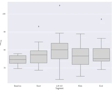
First exploration of HRmax showed that this data was not useable since almost all data points were set at 160 bpm. The scores reported in the following therefore are based on HRavg (see Figure 5). For this measure it could be observed that scores were at a

similar level for all roller coasters (see Figure K1). As for Study 1 responses seemed to be individually different rather than following any pattern (see Figure K2).

HRavg seems to be at the same level before the ride as after it (H1: t(23) = 0.29; p = 0.78). This finding is not dependent on the roller coaster (see Table 4).

Neither does the data support that the HR on the lift hill is higher than during the rest of the session (t(36) = -2.96; p = 0.004); it is rather indicated that HR is lower for this phase. When looking into the results for the single roller coasters this only seems to be the case for Vogel Rok. For the other roller coasters HR is similar for the lift hill as for the rest of the ride.

Finally, it was tested whether the HR was higher during the ride than during the rest of the session. Again the opposite was found (t(29) = -3.87;p = 0.006). A lower HR during the ride was also found for De Vliegende Hollander and Vogel Rok. For the other roller coasters HR remained at the same level as for the other phases.

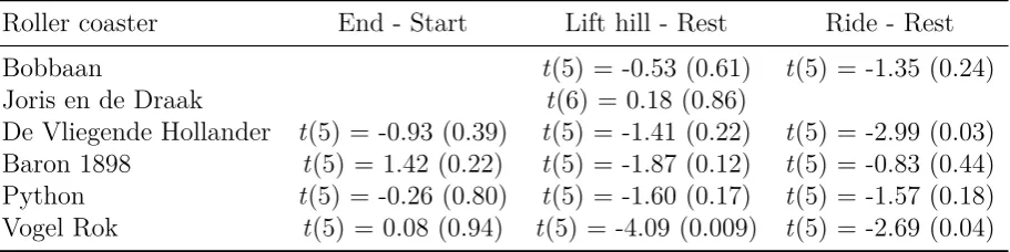
Table 4

Results of the paired t-tests on the average heart rate per roller coaster of the real-world study; p-values are given in brackets.

Roller coaster End - Start Lift hill - Rest Ride - Rest

Bobbaan t(5) = -0.53 (0.61) t(5) = -1.35 (0.24)

Joris en de Draak t(6) = 0.18 (0.86)

De Vliegende Hollander t(5) = -0.93 (0.39) t(5) = -1.41 (0.22) t(5) = -2.99 (0.03)

Baron 1898 t(5) = 1.42 (0.22) t(5) = -1.87 (0.12) t(5) = -0.83 (0.44)

Python t(5) = -0.26 (0.80) t(5) = -1.60 (0.17) t(5) = -1.57 (0.18)

[image:40.595.76.532.635.749.2]

(41)

Figure 5. Box plot of average heart rate for each phase of the real-world study.

EDA

Again responses seemed to be rather individual than pointing to any general effect (see

Figure K4)For the last three phases a flooring effect can be observed (see Figure 6). Additionally, an increase of SCR from the first to the last roller coaster can be observed (see Figure K3).

SCR is at a lower level after the ride than before (t(23) = -2.16; p = 0.04). The same was found for Baron 1898. For the remaining roller coasters number of SCRs was similar before and after the ride (see Table 5).

[image:41.595.103.480.109.411.2]

(42)

rest. This is also found for De Vliegende Hollander and Baron 1898. For the remainder, however, SCR seemed to be on the same level during the lift hill as for the rest.

For the full data set as well as for the single roller coasters arousal during the actual

ride was not higher than during the rest of the video (t(29) = -4.20; p = 0.002; Table 5, respectively); solely, for Bobbaan number of SCR for the ride phase is at the same level as for the other phases. Again it is indicated that SCR is actually lower.

Table 5

Results of the paired t-tests on the number of SCR per minute per roller coaster of the real-world study; p-values are given in brackets.

Roller coaster End - Start Lift hill - Rest Ride - Rest

Bobbaan t(5) = -1.98 (0.10) t(5) = 0.39 (0.71)

Joris en de Draak t(6) = -1.27 (0.25)

Vliegende Hollander t(5) = -1.18 (0.29) t(5) = -2.22 (0.08) t(5) = -2.11 (0.09) Baron 1898 t(5) = -2.50 (0.05) t(5) = -1.37 (0.22) t(5) = -2.38 (0.06)

Python t(5) = -0.37 (0.72) t(5) = -2.87 (0.04) t(5) = -3.87 (0.01)

Vogel Rok t(5) = -0.44 (0.68) t(5) = 0.14 (0.90) t(5) = -2.24 (0.08)

Classification

The SVM reached a accuracy of 32.68 % for the full data set and with a linear kernel. Accuracy was slightly higher for the rbf (34.64 %) and sigmoid (33.33 %) kernels. The

polynomial kernel performed worse with an accuracy of 25.49 % (for all statistics see Table 6).

The tag Hop reached a precision of 72 %, a recall of 75 % and a F1-score of 74 %. Also, did the tag Helix yield a certain degree of good classification (precision = 24 %; recall = 83 %; F1 = 37 %). For the tag Tunnel which was also making up a significant portion of the data (support = 39) all prediction statistics returned zero. The same holds

for the other tags.

(43)

Figure 6. Box plot of number of SCR per minute for each phase of the real-world study.

support below 5 before, were excluded. Also were the variables SDNN, SDSD, RMSSD

and SCRn removed. This resulted in an increase of accuracy to 39.13 % for the linear kernel (rbf: 40.58 %; sigmoid: 39.86 %, poly: 28.26 %).

Prediction statistics for Hop decreased slightly from the first iteration (precision = 69 %; recall = 69 %; F1 = 69 %). ForHelix a even more severe decrease can be observed (precision = 21 %; recall = 8 %; F1 = 11 %). Nevertheless, with the model of the second iteration Tunnel was predicted with a precision of 33 % (recall = 86 %; F1 = 47 %).

(44)

Table 6

Total accuracy, vector magnitude for each variable and event tag support per iteration for data gathered during the real-world study classified with real-world data as training set.

Iteration 1 Iteration 2 Iteration 3

Accuracy 32.64 % 39.13 % 40.00 %

Variable

HRavg 2.0369 2.0189 1.4462

HRmax 2.4821 1.4698 1.0766

HRmin-max 2.2948 1.2376 0.9749

NNavg 4.1971 4.1176 2.7596

SDNN 0.7207

SDSD 0.8680

RMSSD 0.0002

pNN20 2.2558 2.4329 1.4063

pNN50 2.2558 2.4329 1.4063

SCRavg 2.3744 0.7468

SCRn 0.1834

Event tag

Lift hill 9 7

First drop 12 9

Drop 19 18 15

Brake 4

Hop 28 29 22

Tunnel 39 36 43

Helix 35 39 35

Loop 2

Corkscrew 2

Roll 3

Note. Based on linear kernel.

(precision = 32 %; recall = 83 %; F1 = 46 %) remained well, prediction statistics for

Tunnel fell back to zero. Therefore no more variables were removed.

The final combination of variables yielded an accuracy of 33 % on all tags. The same accuracy was found for rbf kernel.

Combined Classification

(45)

for all statistics). Accuracy with the polynomial kernel was slightly inferior at 24.21 %. However, the polynomial SVM outperformed the other three in making predictions for the single elements. The linear model was able to make predictions for two elements: Lift hill (precision = 27 %, recall = 8 %; F1-score = 12 %) andHelix (precision = 26 %, recall = 99 %; F1-score = 41 %). For the same elements the polynomial SVM yielded precision = 20 %, recall = 13 %; F1-score = 16 % and precision = 26 %, recall = 86 %; F1-score

= 39 %, respectively. Furthermore, the polynomial SVM was able to identify First drop (precision = 50 %, recall = 3 %; F1-score = 5 %), Drop(precision = 50 %, recall = 2 %; F1-score = 4 %) andHop (precision = 11 %, recall = 6 %; F1-score = 8 %).

For the second iteration the variables SDNN, SDSD, RMSSD and SCRn were re-moved. This resulted in an accuracy of 25.39 % for all kernels. Even though this was a

small improvement for the rbf and polynomial kernel, the change cancelled out the pre-dictions that could be made with all variables; the only element that was still predicted was Helix (precision = 25 %, recall = 100 %; F1-score = 41 %).

(46)

Table 7

Total accuracy, vector magnitude for each variable and used event tag (x) per iteration as well as event tag support for data gathered during the real-world study classified with VR data as training set.

Iteration 1 Iteration 2 Iteration 3 Iteration 4

Accuracy 25.79 % 25.39 % 28.48 % 28.04 %

Variable

HRavg 2.9069 2.8842 1.8742 1.7993

HRmax 2.5614 2.5591 1.5024 1.4743

HRmin-max 1.7981 1.9317 1.1152 1.0162

NNavg 1.1882 1.0464 0.7851 0.6894

SDNN 0.6903 0.5322 0.5234

SDSD 0.4447 0.2895 0.2596

RMSSD 0.0000 0.0000

pNN20 3.1338 3.2794 1.6533 1.6462

pNN50 2.2170 2.7409 0.9290 0.9049

SCRavg 6.1945 4.8999 4.7051 3.2087

SCRn 0.2314 0.0957

Event tag Support

Lift hill x x x x 39

First drop x x x x 39

Drop x x x x 55

Brake x x 12

Hop x x x x 84

Tunnel x x x x 114

Helix x x x x 129

Loop x x 12

Immelmann x x 6

Corkscrew x x 12

Roll x x 6

Note. Based on linear kernel.

decreased for Hop (precision = 6 %, recall = 2 %; F1-score = 3 %) and cancelled out for

Drop.

For the fourth and last iteration the variables RMSSD and SCRn, which in the

(47)

(precision = 28 %, recall = 100 %; F1-score = 44 %) with this variable combination. When the final variable combination is used for all events accuracy is 25.39 % for all kernels.

Discussion

As for Study 1 it was predicted that arousal after the ride would be higher than before

it and that arousal on the lift hill is higher or, respectively, the arousal during the actual ride is higher than during the rest of the analysed section. Again, neither the first nor one of the latter two could be confirmed. However, unlike for Study 1 no decrease of arousal

over the phases was observed.

Classifications made by the SVM reached mediocre accuracy which increased a good deal when restricting classification to frequent events. Furthermore was data fit better

by a kernel SVM than by a linear SVM. Prediction accuracy for the final model with six variables was close to that of the full model.

Together these findings suggest that real roller coasters have local effects on arousal

that differ between roller coaster elements. These effects, however, do not influence arousal for a prolonged time, so that average arousal in a specific phase of the ride is not increased. Several problems occurred during the collection of the data, which due to the field

situation, were not detected before analysis. First, as seen earlier, HR was only covered up to 160 bpm. This forced a slightly different approach for investigating the replication statements and therefore makes comparison to the first study difficult.

(48)

could have caused inexact anchors for some of the roller coasters.

A less severe but still relevant observation is the increase of SCR from the first to the last roller coaster. This might have happened due to the warm weather on the given day

and the resulting thermoregulatory sweating of the participants. Since for classification SCR is set as a relative value to the baseline, it seemingly becomes relevant from which moment of the day the training data is picked: if the training data is picked from the

morning one element would cause a small number of SCR and therefore the SVM would not recognize the same element at the evening where it would cause more SCR. However, each classification is automatically rerun a number of times with switching, randomly

chosen training sets. We therefore assume that the effect of the increasing SCR was cancelled out. However, future studies could avoid this problem by using times between rides as baseline data instead of only using the beginning of the measured data.

Aside from these points of critique the presented data shows that classification of real-time data is possible. The results could be improved by having all events represented equally often. Furthermore, measures should be taken to prevent motion of the sensors

(49)

General Discussion

The aim of our research was to measure and analyse the physiological effects of virtual as well as real roller coaster rides. For this purpose two different methods of analysis were used. The differences between virtual and real roller coasters in these analyses will be

discussed in the following sections.

Analysis of ride phases

Neither for the real-world nor the VR study did we find the expected effects. Specifically,

it was expected that arousal would increase from the start to the end of a roller coaster ride and that either the lift hill or the actual ride would be the most arousing part of a roller coaster.

These findings indicate that roller coasters do not have a prolonged effect on the passengers. However, it is possible that roller coasters cause short phases of arousal which are cancelled out when looking at the average arousal of longer phases.

That no effect was found strongly contradicts earlier research. Especially, that arousal increases from the beginning of the ride to the end of it has been reported univo-cally (Hinkle, 2016; Kuschyk et al., 2007; Pieles et al., 2017; Rietveld & van Beest, 2007).

For the question whether the lift hill or the ride is most arousing results are mixed in ear-lier research and our studies were not able to introduce more evidence. This is especially striking, seen that the studies by Kuschyk et al. (2007) and Pringle et al. (1989), who

found a clear increase of heart rate during the ride phase, are often cited on the effects of roller coasters. However, from these papers it did not become clear how data was anal-ysed. In replicating the findings we chose for time-normalizing data and therefore used

(50)

these measures might not be the same as those used in earlier studies results might not be comparable.

Remarkably, for both studies our data showed a strong spread between individuals.

This could point towards individual differences that influence arousal caused by roller coasters. As noted earlier (Yamaguchi et al., 2003) observed for individuals who experience roller coasters as enjoyable a decrease of arousal during the ride was observed whereas

for those who experience roller coasters as stressing an increase of arousal during the ride and then again an increase of arousal after the ride was observed. The found spread of individual scores combined with the use of t-tests which can only be used to compare two

moments rather than the full progress, can have caused existing effects to be cancelled out. We therefore suggest to rather use analysis methods which take the whole course into account and to control for effects by subjective experience.

Classification by roller coaster element

Most noticeable, more roller coaster elements could be classified for the real-world study than for the VR study. Furthermore, the classification of the real-world data was more

accurate even though less data was available. However, data from virtual roller coaster rides could be described using less variables than those of the real-world study.

The found pattern in classification could point to differently strong influences by

the factors to arousal noted by Roscoe (1992): emotional, cognitive and physical. As mentioned above, the first part of the roller coaster ride containing the lift hill and first drop has been described causing an emotional response in earlier research since no forces or

(51)

as a training set for the classification of real-world data. This indicates that emotional responses are similar in VR and the real world even though they might not be noticeable with a small sample size. As for cognitive arousal we claimed earlier that it can result from

overcoming sensory discrepancies and the task of retaining spatial presence. In support for this is that for the VR study the SVM was able to discriminate helices, which induce a lateral turn and a roll of the visual field, while it was unable to discriminate hops, which

occurred equally often but only resulted in a slight vertical shift. This indicates that the element which is more complex in its spatial changes causes a stronger response which can not stem from acting forces. For the real-world study, on the other hand, hops could

be classified, pointing towards an effect of the physical forces acting here or at least a stronger effect on emotions and cognition when undergoing this element in the real world. This not only confirms findings by Hinkle (2016), who found the VR roller coasters have

little effect on participants’ arousal, but also those found by Pieles et al. (2017), that stronger g-forces are related to increases of arousal.

Even though the found pattern of arousal can be explained in this way, we must point

to the fact that the exact timing of the tags could not be verified. While imprecision for the VR study should be low, no control was given in the real-world study. As explained above, the starting point of the tagging in the real world was taken from the acceleration data.

However, accelerometers were not calibrated, meaning that one could not say whether acceleration was pointed towards one direction (e.g. upwards when starting to move up the lift hill) or rather uncoordinated (e.g. short shaking of the wrist). Consequently,

Physiological Responses to Roller Coaster Rides: A Pilot Study on the Differences between Virtual Reality and Real World Measures

Contents

Introduction

Study 1

Methods

Results

Discussion

Study 2

Methods

Results

Discussion

General Discussion