Variable Length Input Huffman Coding for System on a Chip Test

Variable-Length Input Huffman Coding for System-on-a-Chip Test

Paul. T. Gonciari, Bashir M. Al-Hashimi, and Nicola Nicolici

Paper no. 556

Accepted for publication as a Transaction Brief Paper

Submitted: July 2002, Revised: October 2002, Final manuscript: January 2003

Paul T. Gonciari and Bashir M. Al-Hashimi

Electronic Systems Design Group

Department of Electronics and Computer Science

University of Southampton

Southampton SO17 1BJ, U.K.

Tel: +44-23-8059-3119 / +44-23-8059-3249 Fax: +44-23-8059-2901

Email: {p.gonciari@zepler.org, bmah@ecs.soton.ac.uk}

Nicola Nicolici

Computer-Aided Design and Test Research Group

Department of Electrical and Computer Engineering

McMaster University

1280 Main St. W., Hamilton, ON L8S 4K1, Canada

Tel: +1-905-525-9140 ext. 27598 Fax: +1-905-521-2922

Email: nicola@ece.mcmaster.ca

Variable-Length Input Huffman Coding for

System-on-a-Chip Test

Abstract

This paper presents a new compression method for embedded core-based system-on-a-chip test. In

addition to the new compression method, this paper analyzes the three test data compression

environ-ment (TDCE) parameters: compression ratio, area overhead and test application time, and explains the

impact of the factors which influence these three parameters. The proposed method is based on a new

Variable-length Input Huffman Coding scheme, which proves to be the key element that determines all

the factors that influence the TDCE parameters. Extensive experimental comparisons show that, when

compared to three previous approaches [1–3], which reduce some test data compression environment’s

parameters at the expense of the others, the proposed method is capable of improving on all the three

1

Introduction

Due to the increased complexity of systems-on-a-chip (SOC), testing is an important factor that drives time-to-market and the cost of the design [4]. In addition to the standard design for test (DFT) issues for SOCs [4], a new emerging problem is the cost of the automatic test equipment (ATE) [5–7]. This is because the cost of ATE grows significantly with the increase in speed (i.e., operating frequency), channel capacity, and memory size [6]. In order to support the large volume of test data with limited channel capacity for future SOCs, the ATE requires modifications and additional expenses. Furthermore, the testing time is also dependent on the volume of test data, thus further increasing the manufacturing cost of the SOCs [7]. The above problems were previously addressed using a external-only approaches (no on-chip overhead is required) or b internal-only approaches (no off-chip interaction is required). The external-only approaches a include test data compaction [8, 9] and methods which reduce the amount of data transfered from the workstation to the ATE [10, 11]. While these approaches effectively reduce the volume of test data, they do not reduce the ATE bandwidth requirements. The internal-only approaches b are based on built-in self-test (BIST), i.e., pseudo-random and/or deterministic BIST. To increase the fault coverage of pseudo-random BIST intrusive techniques such as test point insertion are required [5]. Such techniques are not acceptable in a core-based SOC environment since they lead to a major core redesign effort. In addition, when intellectual property (IP) protected cores are targeted, intrusive techniques cannot be applied. To alleviate the above problems related to pseudo-random BIST, deterministic BIST [12–17] approaches have emerged. These however, may require large on-chip area in order to achieve high test quality. Therefore, test data compression, a test resource partitioning variant [6], arises as a possible solution to reducing the speed, the channel capacity and the memory requirements for ATEs. This solution does not introduce performance penalties and guarantees full reuse of the existing embedded cores as well as the ATE infrastructure, with modifications required during system test preparation (compression) and test application (decompression). Prior work with respect to test data compression is overviewed in the following section.

1.1 Existing approaches to reduce volume of test data

therefore it simplifies the ATE channel capacity and speed requirements. Test data compression methods can reduce the volume of test data applied to the core under test (CUT) or the volume of test responses sent to the ATE. Test response compression is carried out using signature analyzers [18], however, if diagnosis is necessary special schemes may be required [19, 20]. In this paper, we will focus on the former due to the large volumes of test data required to test logic cores, assuming signature analyzers to compress the test output responses. Test data compression methods, which reduce the volume of test data applied to the CUT, can be classified into approaches i which extend deterministic BIST [21–25], ii which exploit the spareness of care bits in the test set [26–28], and iii which exploit the regularities within the test set [1–3, 29–33]. The first category [21–25] i , enhances deterministic BIST approaches, thus alleviating some of their drawbacks (e.g., area overhead, test application time). However, these approaches may suffer from inefficient tester channel usage such as ATE inactivity periods which may increase cost [28]. The second category [26–28] ii , by exploiting care bit spareness, can reduce the volume of test data when the percentage of “don’t care” bits is high. However, it suffers from lock-out situations [12], i.e., the inability of the on-chip decoder to generate a given test pattern, which can degrade test quality, increase test control complexity, as well as negatively influence test application time (TAT). These lock-out situations can increase significantly when the percentage of “don’t care” bits in a test set decreases. Due to these issues the above approaches [26–28] are embedded into the ATPG procedures, which may be prohibited in the IP-based tool flow, where the system integrator cannot access the structural information of the embedded cores. The third category [1–3, 29–33] iii , by exploiting the regularities within the test set, does not require any ATPG re-runs. Since, ATPG procedures require fault simulation, which may be prohibited in IP environments, and long ATE inactivity periods can increase the cost, in this paper we will focus on the third category iii [1–3, 29–33].

Methods which use test set regularities exploit different features of the test set, such as runs of ’0’s, and/or small differences between consecutive test vectors. These methods are based on data compression coding schemes (e.g., run-length, Huffman, Golomb [34]) [1–3, 29, 30] and custom coding schemes [31– 33]. The above coding schemes are implemented using on-chip hardware decoders or on-chip software decoders. With respect to on-chip hardware decoders, Iyengar et al. [29], proposed a new built-in scheme

coding (SC) algorithm was proposed [1]. The method splits the test vectors into fixed-length block size patterns1and applies Huffman coding to a carefully selected subset. In [30], test vector compression is performed using run-length coding. The method relies on the fact that successive test vectors in a test sequence often differ in only a small number of bits. Hence, the initial test set TD is transformed into Tdi f f, a difference vector sequence, in which each vector is computed as the difference between two consecutive vectors in the initial test set. Despite its performance, the method is based on variable-to-fixed-length codes and, as demonstrated in [2], these are less effective than variable-to-variable-length codes. Chandra and Chakrabarty [2] introduced a compression method based on Golomb codes. Both methods, [2] and [30], use the difference vector sequence, hence, in order to generate the initial test set on-chip, a cyclical scan register (CSR) [2, 30] architecture is required. In [3], a new method based on frequency-directed run-length (FDR) codes is proposed. The coding scheme exploits a particular pattern distribution, and by means of experimental results it is shown that the compression ratio can be improved. In [33], a method which exploits the correlation between two consecutive parallel loads into multiple scan chains has been proposed. Since the method uses multiple scan chains it reduces the testing time, however, the extra control signals may negatively influence the compression ratio and control complexity. In addition to the above approaches, which require an on-chip hardware decoder, methods which assume the existence of an embedded processor [31, 32], hence an on-chip software decoder, were also proposed. The method in [31] is based on storing the differing bits between two

test vectors, while the method in [32] uses regular geometric shapes formed only from ’0’s or ’1’s to compress the test data. Regardless of their benefits, in systems where embedded processors are not available or where embedded processors have access only to a small number of embedded cores, these on-chip software decoder based methods are not applicable. A particular advantage of methods which use data compression coding schemes is that they are capable of exploiting the ever increasing gap between the on-chip test frequency and the ATE operating frequency. While in the past this gap has been exploited at the cost of multiple ATE channels [35, 36], hence increasing the bandwidth requirements, approaches which use data compression coding schemes can leverage the frequency ratio without the penalty of extra ATE channels. This is achieved by moving the serialization of test data from the spatial

1_{It should be noted that throughout the paper, a pattern refers to an input pattern used in the coding scheme and not to}

a test pattern. A coding scheme uses fixed-length patterns if all the input patterns have the same length, otherwise, it uses

domain (multiple input channels from the ATE at a low frequency to single scan channel at a high frequency) to the temporal domain (single input channel from the ATE at a low frequency to single scan channel at a high frequency). Hence, data can be fed to the internal cores at their corresponding test frequency without any bandwidth penalty.

1.2 Motivation and contributions

Since so many compression methods have been proposed, an obvious question is why yet another approach is necessary? When analyzed with respect to the three test data compression environment parameters, which are compression ratio, area overhead and test application time, previous approaches trade-off some of the parameters against the others. Therefore, the motivation behind this work is to understand the factors which influence these parameters and to propose a new approach which, when compared to previous approaches, allows simultaneous improvement in compression ratio, area overhead and test application time. This will lead to reduced ATE memory requirements, lower chip area and shorter time spent on the tester, hence reduced test cost. The three main contributions of this paper are:

The test data compression environment (TDCE) comprising the compression method and the on-chip decoder is defined and analyzed with respect to the three TDCE parameters: compression ratio, area overhead and test application time. The interrelation between different factors which influence these parameters is discussed and an analysis of previous work with respect to the TDCE is also given. To the best of our knowledge, this is the first paper which explicitly illustrates the influences of the various factors on the two main components of TDCE (see Section 2);

A new coding scheme, Variable-length Input Huffman Coding (VIHC) is proposed and it is shown that the recently proposed Golomb based method is a particular case of the proposed coding scheme, leading to constantly lower compression ratios. A new compression algorithm comprising a new reordering and a new mapping algorithm is also given;

parallel on-chip decoder are combined, the three test data compression environment parameters can be simultaneously improved with respect to previous work.

The remainder of the paper is organized as follows. Section 2 introduces the test data compression environment and analyzes three previous approaches with respect to its parameters. Section 3 introduces the new Variable-length Input Huffman Coding scheme and illustrates the proposed compression algo-rithm. In Section 4 the proposed on-chip hardware decoder is introduced and the TAT analysis is given. Section 5 and 6 provide the experimental results and conclusions, respectively.

2

Test data compression environment (TDCE)

To better understand how the volume of test data, the area overhead and the testing time can be simultaneously reduced, this section introduces the test data compression environment and characterizes the TDCE with respect to the factors which influence it. Three previous approaches are also analyzed from the TDCE parameters standpoint. Testing in TDCE implies sending the compressed test data from the ATE to the on-chip decoder, decompressing the test data on-chip and sending the decompressed test data to the core under test (CUT). There are two main components in TDCE: the compression method, used to compress the test set off-chip, and the associated decompression method, based on an on-chip decoder, used to restore the initial test set on-chip. The on-chip decoder comprises two units: a unit

to identify a compressed code and a unit to decompress it. If the two units can work independently (i.e., decompressing the current code and identifying a new code can be done simultaneously), then the decoder is called parallel. Otherwise, the decoder is referred to as serial.

2.1 TDCE characterization

Testing in TDCE is characterized by the following three parameters: (a) compression ratio which identifies the performance of the compression method, the memory and channel capacity requirements of the ATE; (b) area overhead imposed by the on-chip decoder (dedicated hardware or on-chip processor); and (c) test application time given by the time needed to transport and decode the compressed test set.

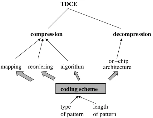
There are a number of factors which influence the above parameters:

on−chip architecture

type length

of pattern of pattern

TDCE

compression decompression

algorithm mapping reordering

coding scheme

Figure 1. TDCE dependency map

the compression algorithm, which based on a coding scheme compresses the initial test set;

the type of input patterns used as input by the coding scheme, which can be of fixed or variable lengths;

the length of the pattern which is the maximum allowed input pattern length used in the coding scheme;

the type of the on-chip decoder, i.e., the on-chip decoder can be serial or parallel.

The relationship between these factors and the two components of the TDCE is illustrated in Fig-ure 1. As it can be seen in the figFig-ure, the coding scheme not only determines the compression factors (i.e., mapping/reordering and compression algorithm), but it also influences the decompression factor (i.e., on-chip architecture). Hence, the coding scheme is a key element that determines the factors that influence the three TDCE parameters, which are discussed next.

(a) Compression ratio: Using patterns of various types and of various lengths, the compression algo-rithms exploit different features of the test set. Mapping and reordering the initial test set emphasizes these features. Therefore, the compression ratio is influenced firstly by the mapping and reordering algo-rithm, and then by the type of input patterns and the length of the pattern, and finally by the compression

(b) Area overhead: Area overhead is influenced firstly by the nature of the decoder, and then by the type of the input pattern and the length of the pattern. If the decoder is serial then the synchronization

between the two units (code identification and decompression) is already at hand. However, if the de-coder is parallel, then the two units have to synchronize, which can lead to increased control complexity and consequently to higher area overhead. Depending on the type of the input pattern different types of logic are required to generate the pattern on-chip. For example, if the coding scheme uses fixed-length input patterns, then a shift register is required to generate the patterns, however, if variable-length in-put patterns (runs of ’0’s for example) are used, then counters can be employed to generate the patterns. Since the length of the pattern impacts the size of the decoding logic, it also influences the area overhead.

(c) Test application time (TAT): TAT is firstly influenced by the compression ratio, and then by the type of the on-chip decoder, and the length of the pattern. To illustrate the factors that influence TAT,

consider the ATE operating frequency as the reference frequency. Minimum TAT (minTAT) is given by the size of the compressed test set in ATE clock cycles. However, this TAT can be obtained only when the on-chip decoder can always process the currently compressed bit before the next one is sent by the ATE. In order to do so, the relation between the frequency at which the on-chip decoder works and the ATE operating frequency has to meet certain conditions. The frequency ratio is the ratio between the on-chip test frequency ( fchip) and the ATE operating frequency ( fate). Consider that the optimum frequency ratio is the frequency ratio for which minTAT is obtained. Since the minTAT is given by the size of the compressed test set, increasing the compression ratio would imply further reduction in TAT. However, this reduction happens only if the optimum frequency condition is met. Since real environments cannot always satisfy the optimum frequency ratio condition, then a natural question is what happens if this condition is not met? TAT in these cases is dependent on the type of on-chip decoder. If the on-chip decoder has a serial nature [2, 3], then the TAT is heavily influenced by changes in the frequency ratio. However, if the decoder has a parallel nature [1], the influences are rather minor. The length of the pattern determines the pattern distribution and at the same time, the number of clock cycles the on-chip

2.2 Analysis of previous approaches in TDCE

In this section three representative previous approaches [1–3] are analyzed from the TDCE parameters standpoint and it is shown that they have improved some of the parameters at the expense of the others.

(i) Selective coding (SC) [1]: This method splits the test vectors into fixed-length input patterns of size b (block size), and applies Huffman coding to a carefully selected number of patterns while the rest of the patterns are prefixed. The SC decoder has a parallel nature. Although, due to this parallelism, the on-chip decoder yields good TAT, the use of fixed-length input patterns and prefixed codes requires shift registers of length b, which lead to large area overhead. In addition, fixed-length input patterns restrain the method from exploiting ’0’-mapped test sets. Hence, special pre-processing algorithms [37, 38] have been proposed to increase the compression attainable with SC. However, these algorithms, which target the SC fixed-length input pattern principle, further increase the computational complexity of this method. It is also interesting to note that using SC with Tdi f f allows good compression when the block size is increased. Hence, due to a fixed-length input pattern the method is restrained from exploiting ’0’-mapped test sets, and the main drawback of this approach is its large area overhead.

(ii) Golomb coding [2]: This method assigns a variable-length Golomb code, of group size mg, to a run of ’0’s. Golomb codes are composed from two parts, a prefix and a tail, and the tail has the length given by log₂mg. Using runs of ’0’s as input patterns, the method has two advantages: firstly the decoder uses counters of length log₂mginstead of shift registers, thus leading to low area overhead; and secondly it exploits the ’0’-mapped test sets improving the compression ratio. Golomb codes are optimum only for a particular pattern distribution, hence the coding scheme yields best compression only in particular cases. Furthermore, since the method in [2] uses a serial on-chip decoder, the TAT is heavily influenced by changes in the frequency ratio. Therefore, the method’s main drawback is its large TAT.

developed to exploit particular pattern distributions common to most test sets yields good compression ratios. However, despite the good compression ratios, having a serial on-chip decoder, large TAT is the main disadvantage of the FDR method.

As illustrated above, current approaches for test data compression efficiently address some of the test parameters at the expense of the others. Therefore, this paper proposes a new coding scheme and a new on-chip decoder, which when combined allow simultaneous improvement in all the three TDCE’s parameters, when compared to previous work.

3

Compression

As illustrated in Section 2.1, the coding scheme is the key component in the TDCE. This section in-troduces a new Variable-length Input Huffman Coding scheme (Section 3.1) and a new compression al-gorithm which combines the new coding scheme with a mapping and reordering alal-gorithm (Section 3.2).

3.1 New Variable-length Input Huffman Coding (VIHC) scheme

The proposed coding scheme is based on Huffman coding. Huffman coding is a statistical data-coding method that reduces the average code length used to represent the unique patterns of a set [34]. It is important to note that the previous approach [1] which uses Huffman coding in test data compres-sion employs only patterns of fixed-length as input to the Huffman coding algorithm. As outlined in the previous section fixed-length input patterns restrict exploitation of the test set features for compres-sion. This problem is overcome by the coding scheme proposed in this section which uses patterns of variable-length as input to the Huffman algorithm, allowing an efficient exploitation of test sets which

exhibit long runs of ’0’s (Section 3). This fundamental distinction does not influence only the compres-sion, but it also provides the justification for employing a parallel decoder using counters (Section 4.1). This will lead not only to significantly lower area overhead, but it will also facilitate TAT reduction when the compression ratio and frequency ratio are increased (see Section 4.2 and 5). The following two examples, illustrate the proposed coding scheme and highlight some interesting properties.

= 26 bits = 16 bits

t_init t_cmp

h m = 4

t cmp

t init 1 01 0000 0000 0000 0001 0000 001

1 011 1

001

000 1 1 010

(a) Initial test vector

L₀ = 1 1 000

L₁ = 01 1 001

L₂ = 001 1 010

L₃ = 0001 1 011

L₄ =0000 4 1

Code Pattern Occurrence

(b) Dictionary L₀ L₁ L₂ L₃ L₄ 0000 0 0 0 1 1 0 1 1 0001 001 1 (2) (2) (4) (8) (1) (4) 01 (1) (1) (1)

(c) Huffman tree

000 001 1 1 1 011 1 010

000 001 1 1 1 011 1 010 1

01

0000 001 0000 0000 0000 0001

VIHC code Golomb code

Run of 0s

(d) Comparison with Golomb for mh 4

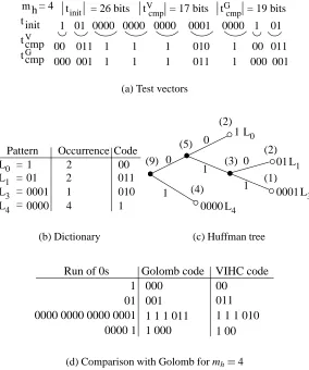
Figure 2. VIHC form_h 4

referred to as patterns (Figure 2(a)). These patterns are used as input to the Huffman coding scheme, where for each pattern the number of occurrences is determined. Having the patterns and the number of occurrences, the first two columns of the dictionary are filled (see Figure 2(b)). Using these two columns, the Huffman tree2is built as explained next (see Figure 2(c)). First, the patterns are ordered in the descending order of their occurrences. Then, the two patterns with the lowest number of occurrences (L0 and L1) are combined into a new node L0 L1

with the number of occurrences given by the sum of the two patterns’ occurrences. This step is repeated until all the nodes are merged into one single node. Initially, patterns L2and L3are merged into L2 L3

, then nodes L0 L1

and L2 L3

are merged together, and finally, node L4 is merged with node L0 L1

L2 L3

. This process is illustrated in Figure 2(c), where the occurrences of the patterns are also given between brackets. After the tree is

created, the Huffman code is obtained by assigning binary ’0’s and ’1’s to each segment starting from the nodes of the Huffman tree (Figure 2(c)). The codes are illustrated in the third column in Figure 2(b). Using the obtained Huffman code, the initial test vector tinit is compressed into tcmp. It should be noted that ordering the patterns in the ascending or descending order of their occurrences does not make any difference to the Huffman tree building algorithm. It is important, however, to always combine the patterns with the smallest number of occurrences.

One interesting property, which can be easily observed when the proposed VIHC scheme and the Golomb coding scheme [2] are compared, is that Golomb codes represent a particular case of VIHCs. This is illustrated in Figure 2(d), where the codes obtained for the runs of ’0’s from tinitin Figure 2(a), are the same for both coding schemes. Because of this particularity, the compression ratios of the Golomb coding scheme will be upper bounded by the compression ratios of the VIHC coding scheme for a given group size. This is illustrated in the following example.

Example 2 Consider the scenario illustrated in Figure 3, where a simple change in the tinit from Fig-ure 2(a) is performed: the 24th bit is set from 0 to 1. The dictionary and the Huffman tree for this new scenario are shown in Figure 3(b) and 3(c) respectively. The Golomb and the VIHC codes for this case are given in Figure 3(d). When tinit is encoded using Golomb coding, the encoded test vector is 19 bits long (t_cmpG ). If the test set is encoded using the proposed VIHC scheme, then the encoded test set is 17 bits long (tV_cmp), which shows the reduction in volume of test data.

In the following we formalize the proposed coding scheme and the properties illustrated using the previous examples. Let mhbe the group size, and L

L0 Lmh

be a set of unique patterns obtained after the test set was divided into runs of ’0’s of maximum length mh. For the computed set of patterns L, the set of number of occurrences P

n0 nmh

is determined. n ∑mh

i 0 Li

ni is the size of the test set, where

Li

denotes the length of pattern Li. The Huffman codes are obtained using L and P. For a pattern Lithe Huffman code is denoted by ci, and the length of the code is given by wi. The minimum codeword length min wi

is referred to as wmin. The size of the compressed test set using a group size of mhis denoted by H mh ∑

mh

i 0

= 26 bits

t_init tV_cmp = 17 bits tG_cmp = 19 bits h

m = 4

t init 1 01 0000 0000 0000 0001 0000 1 01 cmp

tV

1 010 1

011 1 1

00 00 011

cmp tG 1 011 1 001

000 1 1 000 001

(a) Test vectors

L₄ 0000 L₃ L₁ L₀ 1 010 011 00 Code Pattern Occurrence

= ₄

= 0001 1

= 01 2

= 1 2

(b) Dictionary L₀ 0000 0 0 0 1 1 1 0001 01 L₃ L₄ 1 L₁ (1) (2) (2) (3) (5) (4) (9)

(c) Huffman tree

1 1 1 011 001 01 1 000 1 000 0000 1 00 011 1 1 1 010 1 00 0000 0000 0000 0001

Golomb code

Run of 0s VIHC code

(d) Comparison with Golomb for mh 4

Figure 3. VIHC, the general case

There are mh patterns formed from runs of ’0’s ending in 1 (L0 Lmh

1) and one pattern formed from

’0’s only (Lmh) as illustrated in Figure 2(b) for mh 4.

We observed in Example 1 that Golomb coding is a particular case of VIHC. Hence, for a given group size and for a particular pattern distribution the VIHC will reduce to the Golomb code. Consider the following pattern distribution: a nm

h

ni0 ni1 nimh

2

1 distinct i0 imh

2

1

mh and b nk

ni nj

i j k

mh i

j k, where mh represents the group size and ni is the number of occurrences of pattern Li. Based on the above conditions, the Huffman tree illustrated in Figure 4 is constructed. Condition a guarantees that the pattern Lm

h will be the left-most leaf in the tree (as shown

in Figure 4). Condition b ensures that the Huffman tree construction algorithm will merge all the simple patterns first, while the merged patterns are processed afterwards , i.e., it will ensure that the simple patterns (L0 Lmh

0 1

0 1 0 1 0 1 0

1

1 0

0 1

0 1

L_(m h−4) L_(m

h−2) L_(m

h−1) L(mh−3) L_m

h

L₀ L₃ L₂ L₁

Figure 4. Huffman tree when the Golomb code and the VIHC are equal

noted that even if the patterns Li, with i

mh, appear in a different order than the one illustrated in the figure, then as long as the above conditions are met, swapping and rearranging the nodes in the Huffman tree will lead to the tree presented in Figure 4 with no penalties in compression ratio3 [34]. Using the convention that the left leaf of a node is assigned a ’1’ and the right one a ’0’, it is found that cmh 1

and ci 0 followed by i represented on log2mhbits. It is clear that if a run of ’0’s of length lower than mhis compressed, then the code is the same as Golomb’s. If the length of run of ’0’s (l) is greater than mh, then the assigned Golomb code is given by 1 1

l mh

0tail, where tail l _ml

h

represented on log2mh

bits. The same representation is obtained if the code is derived using the proposed VIHC method. Since, the proposed method can produce other codes as well, depending on the pattern distribution for a given group size, the Golomb code is a particular case of the proposed coding method.

It is very interesting to note that the above observation ensures that the VIHC decoder proposed in Section 4.1 can be used to decompress a Golomb compressed test set. Furthermore, if the VIHC coding obtains the same code as Golomb, the minimum code length is 1, or wmin 1. This derives from the previous observation and can be easily seen in Figures 2(c) and 4. Moreover, as illustrated in Figure 3, Golomb coding leads to smaller compression ratios when compared to the proposed VIHC scheme. This is formalized in the following theorem.

3_{It should be noted that when n}

k ni nj in condition

b, the Huffman algorithm may construct a tree different to the

Theorem 1 For a given group size, the compression obtained by the Golomb coding is lower than or

equal to the compression obtained by VIHC.

Proof: The above can be easily shown by using the fact that the Huffman code is an optimal code ([34, Theorem 5.8.1]), i.e., any other code will have the expected length greater than the expected length of the Huffman code. Since the Golomb code is a particular case of VIHC (the VIHC in this particular case is referred to as V IHCG), it is optimal only for a particular pattern distribution. For other pattern distributions the V IHCG code is not optimal, thus the expected length of the V IHCG code is greater. Based on this fact, and using the same reasoning as in [34, Theorem 5.8.1] the proof of the theorem is immediate.

3.2 Compression algorithm based on VIHC

This section presents the compression algorithm which employs the VIHC scheme for compress-ing the test set. In this work, both the compression of the difference vector sequence (Tdi f f) and the compression of the initial test sequence (TD) is taken into account. The initial test set (TD) is partially specified and the test vectors can be reordered. This is because automated test pattern generator (ATPG) tools specify only a small number of bits in every test vector, thus allowing for greater flexibility during mapping. In addition, since full scan circuits are targeted, reordering of test vectors is also allowed.

Algorithm 1VIHC compression

CompressTestSet(TD, compression_type)

begin

i). Prepare initial test set 1. Mapping

SetDefaultValues(TD,compression_type)

2. Reordering TR

D={tmin}, Remove(tmin,TD), previous_solution=tmin

while not TDempty

tmin= DetermineNextVector(TD,compression_type)

if compression_type <> diff then TR

D=TDR tmin

else T_DR=T_DR xortmin

previous_solution

Remove(tmin,TD), previous_solution=tmin

ii). Huffman code computation

L P

=ConstructDictionary(T

R D)

HC=GenHuffmanCode(L,P)

iii).Generate decoder information

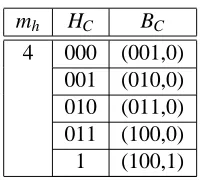
BC=AssociateBinaryCode(HC,mh)

end

i Prepare initial test set: As illustrated in the previous section the VIHC method uses runs of ’0’s as input patterns. The length of these patterns can be increased using this pre-processing procedure. The procedure consists of two steps. In the first step, for the compression of Tdi f f the “don’t cares” are mapped to the value of the previous vector on the same position; for the compression of TD, the “don’t cares” are mapped to ’0’s (SetDefaultValues in Algorithm 1). In the second step the test set is reordered and denoted by T_DR in the algorithm. The reordering process is illustrated in the algorithm in step 2. Starting with the test vector which has the minimum number of ’1’s, the next test vector tmin is determined (procedure DetermineNextVector in the algorithm) such that the following conditions are met. For T_{di f f}, the next test vector is selected such that the number of ’1’s in the difference between the test vector and the previous_solution is minimum, and the length of the minimum run of ’0’s in the difference is maximum (i.e., if there are more test vectors which lead to the same number of ’1’s in the difference with previous_solution, then the one which has the minimum run of ’0’s of maximum length is selected). For TD, the next test vector is selected such that the length of the minimum run of ’0’s is maximum. Further on, if the compression_type is diff, the difference between tmin and the previous solution (previous_solution) is added to the reordered test set (T_DR), otherwise, the selected test vector (tmin) is added to TDR. The reordering algorithm has a complexity of

O

TD

2

, where

TD

mh HC BC

4 000 (001,0)

001 (010,0)

010 (011,0)

011 (100,0)

1 (100,1)

Table 1. Core user/vendor information exchange

the number of test vectors in the test set. The mapping and reordering performed in this procedure will be exploited by the variable-length input patterns used for Huffman code computation in the following procedure.

ii Huffman code computation: Based on the chosen group size (mh) the dictionary of variable-length input patterns L and the number of occurrences P are determined from the reordered test set

(ConstructDictionary in Algorithm 1). This is a mandatory step, because, in contrast to Golomb which has the codewords precomputed for a given group size, VIHC determines the codewords based on the group size and the pattern distribution (i.e., the group size determines the pattern distribution and the pat-tern distribution determines the Huffman codes). Using L and P the Huffman codes (HC) are computed using a Huffman algorithm [34] (GenHuffmanCode in the algorithm). Having determined the Huffman codes, the last procedure generates the information required to construct the decoder.

iii Generate decoder information: This procedure is performed by AssociateBinaryCode in Algo-rithm 1. For each Huffman code cia binary code biis assigned. The binary code is composed from the length of the initial pattern on log2 mh 1

bits and a special bit which identifies the cases when the initial pattern is composed of ’0’s only, or it is a run of ’0’s ending in 1. Thus, bi

Li 0

for i

mh, and bmh

Lm_h

1 (

Li

Timing and synchronization

ATE I/O channel

ATE Memory Test Head

Core Wrapper VIHC

Decoder

Core Wrapper VIHC

Decoder

Core Wrapper VIHC

Decoder

Test Access Mechanism

SoC

Figure 5. VIHC generic decompression architecture based on [2]

4

Decompression

This section introduces the new on-chip VIHC decoder (Section 4.1) for the VIHC scheme and pro-vides the TAT analysis for the proposed decoder (Section 4.2). For the remainder of this paper a generic decompression architecture as shown in Figure 5 is assumed. The VIHC decoder, proposed in Sec-tion 4.1, uses a novel parallel approach in contrast to the previous Golomb [2] serial decoder. It should be noted that for the decompression of Tdi f f, a CSR architecture [2, 30] is used after the VIHC decoder in Figure 5. This work assumes that the ATE is capable of external clock synchronization [36].

4.1 VIHC decoder

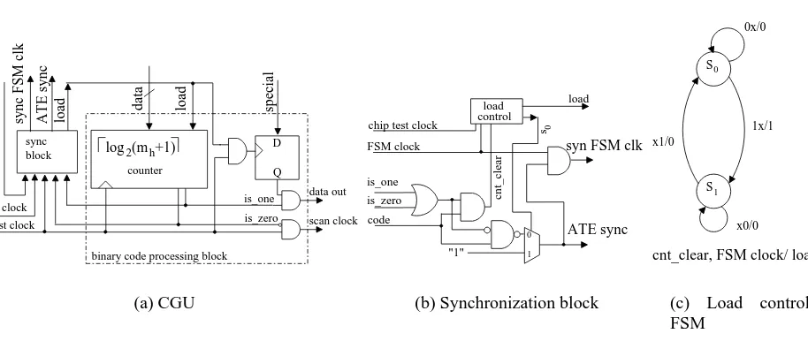
A block diagram of the VIHC decoder is given in Figure 6. The decoder comprises a Huffman de-coder [29] (Huff-dede-coder) and a Control and Generator Unit (CGU). The Huff-dede-coder is a finite state

machine (FSM) which detects a Huffman code and outputs the corresponding binary code. The CGU is responsible for controlling the data transfer between the ATE and the Huff-decoder, generate the initial pattern and control the scan clock for the CUT. The data in line is the input from the ATE synchronous with the external clock (ATE clock). When the Huff-decoder detects a codeword, the code line is high and the binary code is output on the data lines. The special input to the CGU is used to differentiate be-tween the two types of patterns, composed of ’0’s only (Lmh) and runs of ’0’s ending in 1 (L0 Lmh

sync FSM clk

data out

scan clock

chip test clock

code data data in

CGU Huff−decoder (FSM)

special

FSM clock

ATE sync

Figure 6. VIHC decoder

CUT. If the decoding unit generates a new code while the CGU is busy processing the current one, the ATE sync line is low notifying the ATE to stop sending data and the sync FSM clk is disabled forcing

the Huff-decoder to maintain its current state. Dividing the VIHC decoder in Huff-decoder and CGU, allows the Huff-decoder to continue loading the next codeword while the CGU generates the current pattern. Thus, the Huff-decoder is interrupted only if necessary, which is in contrast to the Golomb [2] and the FDR [3] serial decoders. This leads to reduction in TAT when compared to the Golomb and the FDR methods, as it will be shown in Section 5. It should be noted that if the ATE responds to the stop signal with a given latency (i.e., it requires a number of clock cycles before the data stream is stopped or started), the device interface board between the ATE and the system will have to account for this latency using a first in first out (FIFO) - like structure. An additional advantage of the proposed on-chip parallel decoder is that having the two components working in two different clock domains (the Huff-decoder changes state with the ATE operating frequencies, and the CGU generates data at the on-chip test fre-quency), it will leverage the frequency ratio between the on-chip test frequency and the ATE operating frequency. This facilitates data delivery to the CUT at the on-chip test frequency using only one ATE channel, hence using temporal serialization (see Section 1.1) and therefore better resource usage.

The FSM for the Huffman decoder corresponding to the example from Figure 2 is illustrated in Fig-ure 7. Starting from state S1, depending on the value of data in the Huff-decoder changes its state. It is

important to note the following:

after the Huff-decoder detects a codeword it goes back to state S1; for example, if the data in stream is 001 (first bit first) the Huff-decoder first changes its state from S1 to S2 then, from S2 to S3 after which back to S1, and sets data and special to the corresponding binary code ( 010 0

in this case), and the code line high;

S2

S4

S1 S3

data in/data, code, special 0/001, 1, 0

0/011, 1, 0

1/100, 1, 0 1/010, 1, 0

1/xxx, 0, x 0/xxx, 0, x

0/xxx, 0, x

1/100,1,1

Figure 7. FSM for example in Figure 2

D

Q

log₂(m_h+1)

data out scan clock counter is_one is_zero code

chip test clock FSM clock

load

data special

binary code processing block

load

ATE sync

sync FSM clk

block sync (a) CGU s0 "1" controlload is_zero is_one code

syn FSM clk

FSM clock chip test clock

load

cnt_clear

0

1

ATE sync

(b) Synchronization block

S₀ S₁ x1/0 1x/1 x0/0 0x/0

cnt_clear, FSM clock/ load

(c) Load control FSM

Figure 8. CGU for VIHC decoder

example, if the data in stream is 001 (first bit first), the Huff-decoder needs three ATE clock cycles to identify the code;

the Huff-decoder has a maximum of mh states for a group size of mh; the number of states in a Huff-decoder is given by the number of leafs in the Huffman tree minus one; since there are a maximum of mh 1 leafs for a group size of mh, the number of states is mh.

issues to be considered. Firstly, the binary code processing block should be loaded only when a new code is identified; and secondly, the load of new data is done only when the pattern corresponding to the already loaded binary code was fully processed. These tasks are controlled by the synchronization block (sync) illustrated in Figure 8(b). As noted earlier, when the Huff-decoder identifies a code, it will output the associated binary code and set the code line high. When the code line is high, the sync block will determine the values of sync FSM clk, load and ATE sync. The key element in the synchronization block is the load control FSM, whose state diagram is detailed in Figure 8(c). The inputs into the load control FSM are the cnt_clear and the FSM clock. The cnt_clear will notify the FSM when the current code has been processed (i.e., the counter’s value is either zero or one) and there is a new code available (i.e., the code line is high). The FSM clock is used to synchronize the load control FSM with the Huff-decoder FSM. When cnt_clear is 1, the FSM will change to S1and set load to 1. After one clock cycle, the FSM

will set load to 0. If FSM clock is 1, the FSM will return to state S0, otherwise it will remain in state S1.

This last condition was added since a new code can only occur after the FSM clock was 1 (this is how the Huff-decoder is controlled). When the FSM is in state S0, the S0 line in Figure 8(b) together with

the logic behind the multiplexer will ensure that the Huff-decoder continues the load of data from the ATE once the data has been loaded into the binary code processing block. Hence, stopping the stream of data from the ATE to the Huff-decoder only when necessary. The load control FSM can be implemented using one FF and additional logic. The FSM clock signal ensures that the FSM will reach a stable state after one internal clock cycle, therefore it has to be generated as an one internal clock cycle for each external clock cycle period. This can be easily achieved by using the same technique as in [36] for the serial scan enable signal.

When compared to the SC decoder [1], which has an internal buffer and a shift register of size b (the group size), and a Huffman FSM of at least b states, the proposed decoder has only a log2 mh 1

0 0 0 0

0 0 0 0

100 100 100

010 data

h

m = 4 α = 4:1

sync FSM clk ATE clock

chip test clock

pattern 0000 pattern 0000

000 000 100 011 010 001 100 011 010 001 Huff−decoder

CGU

cntr

scan clock load

data out

0 1 2 3 4 5 6 7 8 9

1

data in 1 1

Figure 9. VIHC decoder timing diagram

4.2 Test application time analysis

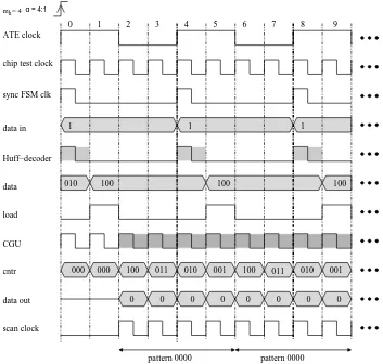
Because the on-chip decoder has two components working in two different clock domains (i.e., the Huff-decoder is receiving data with ATE operating frequencies and the CGU generating data at the on-chip test frequencies), the TAT is influenced by the frequency ratio between the two frequencies: the on-chip test frequencies and the ATE operating frequencies. To understand the effects of the frequency ratio on the TAT, this section provides a TAT analysis with respect to the frequency ratio. It is considered that the data is fed into the Huff-decoder FSM with the ATE operating frequency and that the FSM reaches a stable state after one on-chip test clock cycle. Analyzing the FSM for the Huffman decoder it can be observed that the number of ATE clocks needed to identify a codeword ciis equal to the size of the codeword wi (see Section 3.1). On the other hand, the number of internal clock cycles needed to generate a pattern is equal to the size of the pattern.

described next, Figure 9 shows the timing diagram for a frequency ratio ofα 4, considering mh 4. The diagram corresponds to the generation process of the first two “0000” patterns in Figure 2 (see Example 1 in Section 3.1). This case was chosen to illustrate the parallelism of the proposed VIHC decoder and the overlap between generating the last bit of the pattern and loading the next binary code. The ATE clock, the chip test clock at a ratio of 4 : 1 with respect to the ATE clock, and the sync FSM clk required to drive the Huff-decoder are shown in the upper part of Figure 9. The data in row illustrates the data send from the ATE to the VIHC decoder. As detailed in the previous section, the Huff-decoder reaches a stable state after one internal clock cycle. Hence, the data signals which are loaded into the CGU unit are valid after one internal clock cycle. The time intervals in which the Huff-decoder identifies the last bit of a codeword and outputs the binary code (see Section 4.1) are highlighted in the Huff-decoder row with dashed areas. With the data signals valid, the CGU sets the load signal high

and loads 100 into the counter (cntr row in Figure 9 clock cycle 2). For the next four chip test clock cycles, the CGU is busy generating pattern “0000”, as illustrated in the figure with the dashed areas in row CGU. The cntr is decremented and the data-out outputs the patterns’ bits. While cntr is not zero, the scan clk is generated. At clock cycle 4, the Huff-decoder will identify the next codeword. Again, the load signal is high and the data signals are loaded into the counter. It is important to note that this occurs

simultaneously with the output of the last bit from the previous pattern. Hence, between two consecutive counter loads, forα 4, there are effectively 4 clock cycles in which data can be generated.

Formally, if α f_fchip

ate is the ratio between the on-chip test frequency ( fchip) and the ATE operating

frequency ( fate), then after a Huffman code is identified, α 1 internal clock cycles from the current ATE cycle can be used to generate a pattern. Thus, in order for the Huff-decoder to run without being stopped by the CGU, the CGU has to be able to generate the pattern Liin the number of internal clock cycles remained from the ATE clock in which it was started plus the number of internal clock cycles needed for the Huff-decoder to identify the next codeword. Or,

Li

α 1

1 α wj

1 , where wj is the length of the next codeword in bits. With max

Li

mhand min wi

wmin, the frequency ratio to obtain the smallest TAT is given by αmax

fchip

fate

mh

wmin (optimum frequency ratio). The lowest

TAT is given by H mh

δ, where H mh

time. Thus, an increase in frequency ratio leads to lower test application times when the compression ratio obtained by the proposed VIHC scheme is greater than the one obtained by SC [1], as it will be seen in Section 5.

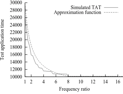
To compute the TAT for the compressed test set for frequency ratios smaller than the optimum fre-quency ratio, an approximation function with respect toα fchip

fate is given next. The function to compute

the TAT for the VIHC decoder in Section 4.1 is given by τ α H mh

δ

mh

∑

i wmin α ni Li

wmin α

α

(1)

when each pattern is followed by the codeword with the lowest decoding time. In order to give an approximation to the above function the pattern distribution is analyzed. For example, for the full scan version of the s5378 ISCAS89 benchmark circuit, Figure 10 illustrates the pattern distribution for mh 16 for the MinTest [39] test set. It can be observed that the patterns with length smaller than 4 and greater than mh 1 are the most frequent. Therefore the function can be approximated with

τ α H mh

δ no

mh wmin α

α

(2)

where nois the number of patterns with length mh(the patterns Lmh 1and Lm

h). It should be noted that

δwill be ignored sinceδ H mh . In the worst case scenario, for no

n mh 1

(each run of length mh is assumed to be followed by a run of length 1)

τ α H mh

n mh 1

mh wmin α

α (3)

0 200 400 600 800 1000 1200 1400 1600

L0 L2 L4 L6 L8 L10 L12 L14 L16

Frequency of occurance

Pattern

Pattern Distribution for s5378

Figure 10. Pattern distribution for s5378 withm_h 16

10000 12000 14000 16000 18000 20000 22000 24000 26000 28000 30000

1 2 4 6 8 10 12 14 16

Test application time

Frequency ratio Simulated TAT Approximation function

Figure 11. TAT for s5378 withm_h 16

5

Experimental results

computed by implementing the SC method and applying it to the MinTest [39] test sets. It should be noted that SC was applied on the same test set as VIHC after the mapping and reordering algorithm proposed in this paper (see Section 3.2). In addition, we have considered the number of patterns used for selective coding as being given by the group size plus one, i.e., for a group size of mh 4, 5 patterns were considered. This is motivated by the pattern distribution obtained with the considered mapping and reordering algorithm which for mh 4 usually leads to the patterns: “0000”, “0001”, “0010”, “0100” and “1000”, as being the most frequent.

Compression ratio Prior to providing a comparison with previous approaches, let’s analyze the per-formances of the proposed method. The experiments performed using the Tdi f f and TD test sets are summarized in Tables 2 and 3 respectively. The tables list, for each ISCAS89 benchmark circuit, the compression ratio obtained for different group sizes (columns 2 to 8), the maximum obtained compres-sion (Max), the size of the maximum compressed test set (H Max ), the size of the initial test set in bits, and the size of the fully compacted MinTest [8] test set. As it can be observed in the tables, the maxi-mum compression ratio is up to 86.83 for circuit s13207 in Table 2, and up to 83.51 for circuit s13207 in Table 3. Analyzing the compression ratios vs. group sizes in the tables, it can be easily observed that the compression ratio tends to increase with the increase in group size. This is illustrated in Figure 12 for circuit s5378. However, after a group size of 16, the increase in compression ratio up to the maximum compression ratio is less than 3%. It is interesting to note that this is contrary to the Golomb [2] com-pression ratio vs. group size trend that tends to have a good comcom-pression ratio for one group size, after which by increasing the group size the compression ratio gets worse. This can be explained by the fact that the particular pattern distribution for which Golomb leads to an optimum code, and hence to good compression, is generally not respected (see Section 3.1).

Compression ratio Size of

Group size Size of Size of MinTest

Circuit 4 6 8 12 14 16 Max HMax Tdi f f [8]

s5378 51.52 54.46 55.23 55.85 56.66 57.33 60.73 9328 23754 20758

s9234 54.84 58.12 58.75 58.45 58.76 59.02 60.96 15332 39273 25935

s13207 69.02 75.90 79.07 82.03 82.69 83.21 86.83 21758 165200 163100

s15850 60.69 65.67 67.48 68.65 68.86 68.99 72.34 21291 76986 57434

s35932 40.35 49.92 56.97 61.08 62.54 66.47 71.91 7924 28208 19393

s38417 54.51 58.57 59.96 60.86 61.22 61.98 66.38 55387 164736 113152

s38584 56.97 61.21 62.50 63.01 63.00 62.97 66.29 67114 199104 104111

Table 2. VIHC forT_{di f f}

Compression ratio Size of

Group size Size of Size of MinTest

Circuit 4 6 8 12 14 16 Max HMax TD [8]

s5378 41.13 42.15 42.85 44.85 45.73 46.94 51.78 11453 23754 20758

s9234 45.27 46.14 45.27 46.14 46.02 46.14 47.25 20716 39273 25935

s13207 67.60 74.12 76.92 79.49 80.03 80.36 83.51 27248 165200 163100

s15850 58.01 62.43 63.73 64.42 64.28 64.06 67.94 24683 76986 57434

s35932 29.76 38.73 44.24 47.07 47.89 51.84 56.08 12390 28208 19393

s38417 37.19 40.45 43.78 46.97 47.34 47.79 53.36 76832 164736 113152

s38584 54.43 57.89 58.81 58.90 59.17 59.62 62.28 75096 199104 104111

Table 3. VIHC forT_D

35 40 45 50 55 57.33 60.73

2 16 20 40 100 201

Compression ratio

Group size

Figure 12. Compression ratio vs. group size for s5378 withT_{di f f}

Tdi f f TD

SC Golomb FDR SC Golomb FDR

Circuit [1] [2] TR

D [3] TDR VIHC [1] [3] TDR [3] TDR VIHC

s5378 52.33 40.70 51.00 48.19 59.00 60.73 43.64 37.11 37.13 48.02 48.03 51.78

s9234 52.63 43.34 58.08 44.88 58.85 60.96 40.04 45.25 45.27 43.59 43.53 47.25

s13207 77.73 74.78 82.34 78.67 85.50 86.83 74.43 79.74 79.75 81.30 81.30 83.51

s15850 63.49 47.11 66.58 52.87 71.02 72.34 58.84 62.82 62.83 66.22 66.23 67.94

s35932 65.72 N/A 23.28 10.19 49.78 71.91 64.64 N/A N/A 19.37 19.36 56.08

s38417 57.26 44.12 56.72 54.53 64.32 66.38 45.15 28.37 28.38 43.26 43.26 53.36

s38584 58.74 47.71 61.20 52.85 65.27 66.29 55.24 57.17 57.17 60.91 60.92 62.28

Table 4. Best compression comparison

for the remainder of this paper. Since, as illustrated in Figure 12, the increase in compression ratio for group sizes larger than 16 is small (less than 3% on average), further on the maximum group size for all the comparisons is considered 16.

Tdi f f TD

Group SC Group SC

Circuit size [1] VIHC size [1] VIHC

s5378 12 52.33 55.85 12 43.64 44.85

s9234 10 52.63 58.79 8 40.04 45.27

s13207 16 77.73 83.21 16 74.43 80.36

s15850 16 63.49 68.99 16 58.84 64.04

s35932 16 65.72 66.47 16 64.64 51.84

s38417 12 57.26 60.86 10 45.15 45.25

s38584 14 58.74 63.00 12 55.24 58.90

Table 5. Comparison between SC and VIHC

Tdi f f TD

Group Golomb Group Golomb

Circuit size T_DR VIHC size T_DR VIHC

s5378 8 51.00 55.23 4 37.13 41.13

s9234 8 58.08 58.75 4 45.27 45.27

s13207 16 82.34 83.21 16 79.75 80.36

s15850 8 66.58 67.48 8 62.83 63.73

s35932 4 23.28 40.35 4 N/A 29.76

s38417 8 56.72 59.96 4 28.38 37.19

s38584 8 61.20 62.50 8 57.17 58.81

Table 6. Comparison between Golomb and VIHC

that for a given group size the proposed compression method yields better compression ratios, and hence it exploits better the test set than the previous approaches. It should be noted that in the case of SC, better results might be obtained at the cost of extra computational complexity if other mapping algorithms are used. In the following an area overhead comparison between the proposed on-chip decoder and the three previously proposed on-chip decoders (SC [1], Golomb [2], FDR [3]) is given.

Compression Area overhead in tu

Method Group size

4 8 16

SC [1] 349 587 900

Golomb [2] 125 227 307

FDR [3] 320

VIHC 136 201 296

technology units for the lsi10k library (Synopsys Design Compiler)

Table 7. Area overhead comparison for s5378

decoder [2] has lower area overhead for a group size of 4, when compared to the proposed decoder, by increasing the group size the area overhead of the Golomb’s decoder is greater than the proposed one’s. This is because, in order to decode the tail part of the code, the Golomb decoder basically implements the behavior of a counter within the Golomb FSM. It should be noted that for the case when the Tdi f f test set is used, a CSR architecture is required. Since the CSR has to be of the length of the scan chain fed by the decoder, the CSR overhead is dominated by the length of the internal scan chain of the targeted core (e.g., for core s5378 the CSR comprises 179 scan cells), being independent of the chosen compression method. Hence, a CSR is needed by all four approaches and therefore not considered in the area over-head comparison given in Table 7. In addition, it has been shown in [30] how the internal scan chains of neighbouring cores in a SOC can be used to eliminate the need for the CSR. The comparisons provided until now show that the proposed method improves on the first two TDCE parameters: compression ratio and area overhead. In the following, the last parameter, the TAT, is compared with the previous work.

Circuit Comp. TAT (ATE clock cycles) for Tdi f f TAT (ATE clock cycles) for TD

Method α 2 α 4 α 6 α 8 α 2 α 4 α 6 α 8

s5378 MinTest [8] 20758 20758

SC [1] 15835 12412 11323 11323 17259 14323 13387 13387

Golomb [2] 20649 16020 13782 13782 23529 19232 14935 14935

FDR [3] 22263 14678 12968 11679 24933 16803 15259 14039

VIHC 15868 11569 10777 10137 17668 13740 12914 12782

s9234 MinTest [8] 25935 25935

SC [1] 24815 20675 18605 18605 27459 23547 23547 23547

Golomb [2] 31186 23555 19894 19894 35580 28537 21494 21494

FDR [3] 36135 24128 21381 19001 42066 29206 26675 24086

VIHC 24895 17994 16905 16095 27235 23860 21154 21154

s13207 MinTest [8] 163100 163100

SC [1] 89368 53490 45137 36784 91369 57455 49847 42239

Golomb [2] 104440 66381 47783 47481 106169 69190 51272 50847

FDR [3] 107059 63011 49858 41989 116101 70361 57089 48538

VIHC 89865 52769 44180 36065 90920 55229 47319 40048

s15850 MinTest [8] 57434 57434

SC [1] 47256 33844 30975 28106 47186 35432 31687 31687

Golomb [2] 57860 41452 33442 33442 64730 48528 32326 32326

FDR [3] 62419 39628 33767 29488 65020 42270 36732 32362

VIHC 47366 32513 29437 26692 48169 34735 31055 30871

s35932 MinTest [8] 19393 19393

SC [1] 16870 11749 10710 9671 16879 11932 10780 9974

Golomb [2] 31758 26699 21640 21640 42267 38341 34415 34415

FDR [3] 32509 20605 18438 17045 42159 27468 25893 24821

VIHC 17584 12076 10857 9645 19908 15641 14670 13736

s38417 MinTest [8] 113152 113152

SC [1] 105076 78851 70403 70403 116282 98849 90354 90354

Golomb [2] 136554 103140 86974 86974 177074 147530 117986 11798

FDR [3] 144811 93450 81578 73182 186261 123700 113451 10521

VIHC 104642 74293 67940 62625 118989 92777 87914 87002

s38584 MinTest [8] 104111 104111

SC [1] 125141 97892 90020 82148 126309 98019 89124 89124

Golomb [2] 156238 115731 96073 96073 161236 122107 103200 10320

FDR [3] 170143 110982 96677 85687 179530 118628 104630 93260

VIHC 126969 92632 83130 82582 127849 92377 85783 80392

the core under test, hence the size of the test set in bits. Analyzing columns 3 to 6 and 7 to 10, it can be observed that in general for small frequency ratios the SC has slightly better TAT than the proposed method (e.g., s5378, s15850 and s38584 withα 2 for both Tdi f f and TD). However, generally the TATs of the proposed method are better than the ones of the previous methods (SC [1], Golomb [2], FDR [3]). Exception makes the circuit s35932 in the case of SC. This is because the minimum codeword (wmin) (see Section 4.2) for SC is 2 and wminfor VIHC is 1, and the compression ratio obtained by SC is almost equal to VIHC’s in the case of T_{di f f}, and greater than VIHC’s in the case of TD. These two combined lead to smaller TAT in this case. The reduction in TAT when compared to previous methods is detailed next. It can be observed that overall, in comparison to SC, TAT reduction of up to 12% is obtained for Tdi f f (e.g., in the case of circuit s9234 forα 4). Similarly for TD, the TAT is reduced by up to 10% when compared to SC (e.g., in the case of circuit s9234 for α 6). When compared to Golomb and FDR, for the Tdi f f test set, TAT reductions up to 54% and 45% are obtained in the case of circuit s35932. For TD, the TAT reduction is as high as 59% and 43% for Golomb and FDR respectively. For the rest of the circuits, in the case of Tdi f f, the TAT ranges from similar values (when frequency ratio increases) to reduction of up to 27% when compared to Golomb (s38417), and reduction of up to 31% when com-pared to FDR (s9234). The same applies for TD, where the TAT reduction is up to 26% (s38417) when compared to Golomb, and up to 36% (s38417) when compared to FDR. Comparing the TAT with the one obtained by MinTest [8] gives an idea on how the TAT behaves for different frequency ratios when compared to fully compacted test sets. As it can be easily seen in the table, when compared to MinTest, the TAT is reduced as much as 77% for the circuit s13207 in the case of Tdi f f for a frequency ratio of α 8. Similarly for TDin the case of circuit s13207, TAT reduction up to 77% is obtained forα 8. It should be noted that MinTest should improve its TAT if serialization buffers are introduced between the ATE and the SOC. However this implies the use of multiple ATE channels for one scan channel, which is avoided by the proposed approach.

SC[1] Golomb[2] FDR[3] VIHC

Compression X X

Area overhead X X

Test application time X X

Table 9. Previous approaches compared to VIHC

area overhead when compared to VIHC at the expense of lower compression ratio and higher TAT. SC [1], on the other hand, has overall comparable TAT when compared to VIHC. However, this is achieved at a very high penalty in area overhead which is the main shortcoming of the parallel decoder based on fixed-length Huffman coding.

6

Concluding remarks

This paper has presented a new compression method called Variable-length Input Huffman Coding (VIHC). This paper also provides a taxonomy on the factors which influence the three test data com-pression environment parameters: comcom-pression ratio, area overhead and test application time. Unlike previous approaches [1–3] which reduce some test parameters at the expense of the others, the proposed compression method is capable of minimizing all the three test data compression parameters simulta-neously. This is achieved by accounting for multiple interrelated factors that influence the results, such as pre-processing the test set, the size and the type of the input patterns to the coding algorithm, and the type of the decoder. The results in Section 5 show that the proposed method obtains constantly bet-ter compression ratios than [1–3]. Furthermore, by exploiting the variable-length input approach, great savings in area overhead are achieved (up to threefold reduction when compared to the fixed-length ap-proach [1]). Moreover, the parallel decoder leads to significant savings in TAT when compared to the serial decoders [2, 3]. Thus, this paper has shown that the proposed method decreases the ATE memory and channel capacity requirements by obtaining good compression ratios, and reduces TAT through its parallel on-chip decoder with low area overhead.

References

[1] A. Jas, J. Ghosh-Dastidar, and N. A. Touba, “Scan Vector Compression/Decompression Using Sta-tistical Coding,” in Proceedings IEEE VLSI Test Symposium (VTS), pp. 114–121, IEEE Computer Society Press, Apr. 1999.

[2] A. Chandra and K. Chakrabarty, “System-on-a-Chip Test Data Compression and Decompression Architectures Based on Golomb Codes,” IEEE Transactions on Computer-Aided Design, vol. 20, pp. 113–120, Mar. 2001.

[3] A. Chandra and K. Chakrabarty, “Frequency-Directed Run-Length (FDR) Codes with Application to System-on-a-Chip Test Data Compression,” in Proceedings IEEE VLSI Test Symposium (VTS), pp. 114–121, IEEE Computer Society Press, Apr. 2001.

[4] E. J. Marinissen, Y. Zorian, R. Kapur, T. Taylor, and L. Whetsel, “Towards a Standard for Embed-ded Core Test: An Example,” in Proceedings IEEE International Test Conference (ITC), (Atlantic City, NJ), pp. 616–627, IEEE Computer Society Press, Sept. 1999.

[5] G. Hetherington, T. Fryars, N. Tamarapalli, M. Kassab, A. Hassan, and J. Rajski, “Logic BIST for Large Industrial Designs: Real Issues and Case Studies,” in Proceedings IEEE International Test Conference (ITC), (Atlantic City, NJ), pp. 358–367, IEEE Computer Society Press, Sept. 1999.

[6] Y. Zorian, S. Dey, and M. Rodgers, “Test of Future System-on-Chips,” in Proceedings International Conference on Computer-Aided Design (ICCAD), (San Jose, CA), pp. 392–398, Nov. 2000.

[7] J. Rajski, “DFT for High-Quality Low Cost Manufacturing Test,” in Proceedings of the Asian Test Symposium (ATS), (Kyoto, Japan), pp. 3–8, IEEE Computer Society Press, Nov. 2001.

[8] I. Hamzaoglu and J. H. Patel, “Test set compaction algorithms for combinational circuits,” in Pro-ceedings International Conference on Computer-Aided Design (ICCAD), pp. 283–289, Nov. 1998.

[10] T. Yamaguchi, M. Tilgner, M. Ishida, and D. S. Ha, “An efficient method for compressing test data to reduce the test data download time,” in Proceedings IEEE International Test Conference (ITC), pp. 79–88, IEEE Computer Society Press, 1997.

[11] M. Ishida, D. S. Ha, and T. Yamaguchi, “Compact: A hybrid method for compressing tets data,” in Proceedings IEEE VLSI Test Symposium (VTS), pp. 62–69, IEEE Computer Society Press, Apr. 1998.

[12] B. Koenemann, “LFSR-Coded Test Patterns for Scan Designs,” in Proceedings IEEE European Test Conference (ETC), pp. 237–242, IEEE Computer Society Press, Mar. 1991.

[13] H.-J. Wunderlich and G. Kiefer, “Bit-Flipping BIST,” in Proceedings International Conference on Computer-Aided Design (ICCAD), (San Jose, CA), Nov. 1996.

[14] N. A. Touba and E. J. McCluskey, “Altering a Pseudorandom Bit Sequence for Scan-Based BIST,” in Proceedings IEEE International Test Conference (ITC), (Washington, DC), pp. 167–175, IEEE Computer Society Press, Oct. 1996.

[15] G. Kiefer and H.-J. Wunderlich, “Deterministic BIST with Multiple Scan Chains,” in Proceedings IEEE International Test Conference (ITC), (Washington, DC), pp. 1057–1064, IEEE Computer

Society Press, Oct. 1998.

[16] J. Rajski, J. Tyszer, and N. Zacharia, “Test data decompression for multiple scan designs with boundary scan,” IEEE Transactions on Computers, vol. 47, pp. 1188–1200, Nov. 1998.

[17] G. Kiefer, H. Vranken, E. J. Marinissen, and H.-J. Wunderlich, “Application of Deterministic Logic BIST on Industrial Circuits,” in Proceedings IEEE International Test Conference (ITC), (Atlantic City, NJ), pp. 105–114, IEEE Computer Society Press, Oct. 2000.

[18] M. L. Bushnell and V. D. Agrawal, Esentials of Electronic Testing for Digital, Memory and Mixed-Signal VLSI Circuits. Kluwer Academic OPTpublishers, 2000.