DOI 10.1007/s12083-009-0062-6
Decentralising a service-oriented architecture
Jan Sacha·Bartosz Biskupski·Dominik Dahlem· Raymond Cunningham·René Meier·Jim Dowling· Mads Haahr
Received: 7 January 2009 / Accepted: 22 September 2009
© The Author(s) 2009. This article is published with open access at Springerlink.com
Abstract Service-oriented computing is becoming an
increasingly popular paradigm for modelling and build-ing distributed systems in open and heterogeneous environments. However, proposed service-oriented ar-chitectures are typically based on centralised compo-nents, such as service registries or service brokers, that introduce reliability, management, and performance issues. This paper describes an approach to fully de-centralise a service-oriented architecture using a self-organising peer-to-peer network maintained by service providers and consumers. The design is based on a gra-dient peer-to-peer topology, which allows the system to replicate a service registry using a limited number of the most stable and best performing peers. The paper eval-uates the proposed approach through extensive sim-ulation experiments and shows that the decentralised registry and the underlying peer-to-peer infrastructure scale to a large number of peers and can successfully manage high peer churn rates.
Keywords Gradient topology·
Service-oriented architecture·Super-peer election· Utility·Aggregation
J. Sacha (
B
)Vrije Universiteit, Amsterdam, The Netherlands
e-mail: [email protected]
B. Biskupski·D. Dahlem·R. Cunningham· R. Meier·M. Haahr
Trinity College, Dublin, Ireland J. Dowling
Swedish Institute of Computer Science, Kista, Sweden
1 Introduction
Service-Oriented Computing (SOC) is a paradigm where software applications are modelled as collections of loosely-coupled, interacting services that communi-cate using standardised interfaces, data formats, and access protocols. The main advantage of SOC is that it enables interoperability between different software ap-plications running on a variety of platforms and frame-works, potentially across administrative boundaries [1, 2]. Moreover, SOC facilitates software reuse and automatic composition and fosters rapid, low-cost de-velopment of distributed applications in decentralised and heterogeneous environments.
A Service Oriented Architecture (SOA) usually con-sists of three elements: service providers that publish and maintain services, service consumers that use ser-vices, and a service registry that allows service discov-ery by prospective consumers [1,3]. In many proposed SOAs, the service registry is a centralised component, known to both publishers and consumers, and is often based on the Universal Description Discovery and In-tegration (UDDI) protocol.1Moreover, many existing SOAs rely on other centralised facilities that provide, for example, support for business transactions, service ratings or service certification [3].
However, each centralised component in a SOA con-stitutes a single point of failure that introduces security and reliability risks, and may limit a system’s scalability and performance.
This paper describes an approach to decentralise a service-oriented architecture using a self-organising
Peer-to-Peer (P2P) infrastructure maintained by ser-vice providers and consumers. A P2P infrastructure is an application-level overlay network, built on top of the Internet, where nodes share resources and provide services to each other. The main advantages of P2P systems are their very high robustness and scalability, due to inherent decentralisation and redundancy, and the ability to utilise large amounts of resources avail-able on machines connected to the Internet. While the service provision and consumption in a SOA are inher-ently decentralised, as they are usually based on direct interactions between service providers and consumers, a P2P infrastructure enables the distribution of a service registry, and potentially other SOA facilities, across sites available in the system.
However, the construction of P2P applications poses a number of challenges. Measurements on deployed P2P systems show that the distributions of peer charac-teristics, such as peer session time, available bandwidth or storage space, are highly skewed, and often heavy-tailed or scale-free [4–7]. A relatively small fraction of peers possess a significant share of the system re-sources, and a large fraction of peers suffer from poor availability or poor performance. The usage of these low stability or low performance peers for providing system services (e.g., routing messages on behalf of other peers) can lead to a poor performance of the entire system [8]. Furthermore, many distributed al-gorithms, such as decentralised keyword search [9], become very expensive as the system grows in size due to the required communication overhead.
As a consequence, P2P system designers attempt to find a trade-off between the robustness of fully decen-tralised P2P systems and the performance advantage and manageability of partially centralised systems. A common approach is to introduce a two-level hierarchy of peers, where so called super-peers maintain system data and provide core functionality, while ordinary peers act as clients to the super-peers.
In this paper, a service registry is distributed between service providers and consumers in the system using a gradient-based peer-to-peer topology. The application of a gradient topology allows the system to place the SOA registry on a limited number of the most reliable and best performing peers in order to improve both the stability of the service registry and the cost of searching using this registry. Furthermore, the gradient topology allows peers to update and optimise the set of registry replicas as the system and its environment evolve, and to limit the number of replica migrations in order to reduce the associated overhead. Analogously, the gra-dient topology can be used to decentralise additional
facilities in a SOA, such as a transaction service or a certificate repository.
The proposed approach has been evaluated in a number of usage scenarios through extensive simula-tion experiments. Obtained results show that the de-centralised registry, and the underlying algorithms that maintain the gradient topology, are scalable and re-silient to high peer churn rates and random failures.
The remainder of this paper is organised as follows. Section2describes the design of a gradient P2P topol-ogy and shows how this topoltopol-ogy is used to support a decentralised service registry. Section 3contains an extensive evaluation of a decentralised service registry built top of a gradient topology. Section4describes the review of related work, and Section 5 concludes the paper.
2 Gradient topology
The gradient topology is a P2P overlay topology, where the position of each peer in the system is determined by the peer’s utility. The highest utility peers are clustered in the centre of the topology (the so called core) while peers with lower utility are found at gradually increas-ing distance from the centre. Peer utility is a metric that reflects the ability of a peer to contribute resources and maintain system infrastructural services, such as a SOA registry.
The gradient topology has two fundamental proper-ties. Firstly, all peers in the system with utility above a given value are connected and form a gradient sub-topology. Such high utility peers can be exploited by the system for providing services to other peers or hosting system data. Secondly, the structure of the topology enables an efficient search algorithm, called gradient search, that routes messages from low utility peers towards high utility peers and allows peers to discover services or data in the system. These two properties contribute to an efficient implementation of a decen-tralised SOA registry.
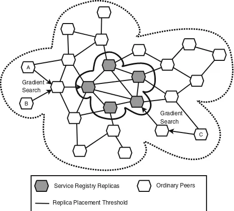
The SOA registry is distributed between a number of peers in the system for reliability and performance reasons. Hence, there are two types of peers: super-peers that host registry replicas, and ordinary super-peers that do not maintain any replicas. A utility thresh-old is defined as a criteria for the registry replica placement, i.e., all peers with utility above a selected threshold host replicas of the registry. Finally, gra-dient search is used by ordinary peers to discover high utility peers that maintain the registry. Figure 1
Gradient Search
Service Registry Replicas Ordinary Peers Gradient
Search A
B
C
[image:3.595.51.289.54.269.2]Replica Placement Threshold
Fig. 1 Registry replication and discovery in the gradient topol-ogy. Peers A, B, and C access registry replicas, hosted by peers in the core, using gradient search
service registry is located at the core peers determined by the replica placement threshold.
The following subsections describe in more detail the main components of the gradient topology: utility met-rics that capture individual peer capabilities; a neigh-bour selection algorithm that generates the gradient topology; a super-peer election algorithm for registry replica placement; an aggregation algorithm, required by the super-peer election, that approximates global system properties; a gradient search heuristic that en-ables the discovery of registry replicas; and finally, the registry replica synchronisation algorithms.
2.1 Characterising peers
In order to determine peers with the most desired characteristics for the maintenance of a decentralised service, such as the SOA registry, a metric is defined that describes the utility of peers in the system. Peer utility, denoted U(p)for peer p, is a function of local peer properties, such as the processing performance, storage space, bandwidth, and availability. Most of these parameters can be measured, or obtained from the operating system, by each peer in a straight-forward way. In the case of dynamically changing parameters, a peer can calculate a running average.
Network characteristics, such as bandwidth, latency, and firewall status, are more challenging to estimate due to the decentralised and complex nature of wide-area networks. Moreover, many network properties, including bandwidth and latency, are properties of pairs of peers, i.e., connections between two peers, rather than individual peers. Nevertheless, a peer can estimate the average latency and bandwidth of all its connections over time and use the average value as a general in-dication of its network connectivity and overall utility for the system. Furthermore, it has been shown that the bottleneck bandwidth of a connection between a peer and another machine on the Internet is often deter-mined by the upstream bandwidth of the peer’s direct link to the Internet [10]. Thus, available bandwidth can be treated as a property of single peers.
Peer stability is amongst the most important peer characteristics, since in typical P2P systems the session times vary by orders of magnitude between peers, and only a relatively small fraction of peers stay in the system for a long time [8]. One way of measuring the peer stability is to estimate the expected peer session duration using the history of previous peer session times. Stutzbach et al. [7] show that subsequent sess-ion times of a peer are highly correlated and the dura-tion of a previous peer session is a good estimate for the following session duration. However, the information about previous peer session durations may not always be available, for example for new peers that are joining the system for the first time. Another approach is to estimate the remaining peer session time using the cur-rent peer uptime. Stutzbach et al. [7] show that current uptime is on average a good indicator of remaining up-time, although it exhibits high variance. For example, in systems where the peer session times follow the power-law (or Pareto) distribution, the expected remaining session time of a peer is proportional to the current peer uptime. Similar properties can be derived for other session time distributions, such as the Weibull or log-normal distributions, used in P2P system modelling.
Formally, if the peer session times in a system follow the Pareto distribution, the probability that a peer ses-sion duration, X, is greater than some value x is given by P(X>x)=(mx)k, where m is the minimum session
duration and k is a system constant such that k>1. The expected peer session duration is E(X)=μ= kk−·m1. However, if a peer’s current uptime is u, where u>m, the expected session duration follows the Pareto distri-bution with the minimum value of u, i.e., P(X>x)=
(u x)
k, and hence, the expected session duration time is k·u
k−1. From this we can derive the expected remaining
2.2 Utility metric properties
The choice of the utility metric has a strong impact on the gradient topology. A utility metric where peers frequently changes their utility values puts more stress on the neighbour selection algorithm and may desta-bilise the topology. It may also cause frequent switches between super-peers and ordinary peers, which may be expensive and undesired.
However, if peer utility grows or decreases monoton-ically, peers can cross the super-peer election threshold only once, assuming a constant threshold. Additionally, if the utility changes are predictable, each peer is able to accurately estimate its own utility and the utility of its neighbours at any given time.
For example, if peer p defines its utility as the ex-pected session duration, Ses(p), and estimates it based on the history of its previous sessions, utility U(p) is constant during each peer session. When p is elected a super-peer, it is not demoted to a client unless the super-peer election threshold increases above U(p).
If the utility of p is defined as p’s current uptime, denoted U p(p), peer utility increases monotonically with time. Again, when p is elected a super-peer, it is not demoted unless the election threshold rises above U p(p). More importantly, the utility function is fully predictable. Any peer q, at any time t, can compute the utility of p, given q has a knowledge of p’s birth time, i.e., the time tpwhen peer p entered the system. Peer
utility is simply equal to
U(p)=t−tp. (1)
Clocks do not need to be synchronised between peers, and q can estimate the birth time of p using its own clock. At time t, when q receives the current uptime U p(p)from p, it assumes that tp=t−U p(p).
For capacity metrics, such as the storage, band-width, or processing capacity, there are two general approaches to define peer utility. One approach is to calculate peer utility based on the currently available peer capacity. However, this has the drawback that peer utility may change over time, and these changes may be unpredictable to other peers. A better approach is to define peer utility based on the total peer capacity, which is usually static. Such utility functions are ad-dressed later in the super-peer election Section2.4.
Finally, certain algorithms described in this article assume that peer utility values are unique, i.e., U(p)= U(q)for any peers p=q. This property may not hold for some utility definition, particularly if peer utility is based on hardware parameters such as CPU clock speed and amount of RAM. If the utility function is
significantly coarse-grained, the construction of a gra-dient topology may become impossible. In order to address this problem, each peer can add a relatively small random number to its utility value to break the symmetry with other peers.
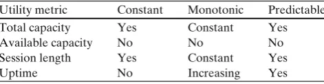
Table1summarises the utility metric properties.
2.3 Generating a gradient peer-to-peer topology
In P2P systems, each peer is connected to a limited number of neighbours and the system topology is deter-mined by the neighbourhood relation between peers.
There are two general approaches to modelling and implementing the neighbourhood relation between peers. In the first approach, a peer stores addresses of its neighbours, which allows the peer to send mes-sages directly to each neighbour, and the neighbour-hood relation is asymmetric. This strategy is relatively straightforward to implement, but it has the drawback that peers may store stale addresses of peers that have left the system. This is especially likely in the presence of heavy churn in the system. Moreover, such dangling references can be disseminated between peers unless an additional mechanism is imposed that eliminates them from the system, such as timestamps [11,12].
[image:4.595.307.543.657.718.2]In the second approach, the neighbourhood relation between peers is symmetric. This can be simply im-plemented by maintaining a direct, duplex connection (e.g., TCP) between each pair of neighbouring peers. If a peer is not able to maintain connections with all its neighbours, for example due to the operating system limits, neighbouring peers store the addresses of each other. This has the advantage that peers can notify each other when changing their neighbourhoods or leaving the system, which helps to keep the neighbourhood sets up to date. Furthermore, outdated neighbour en-tries are not propagated between peers in the system, as each peer verifies a reference received from other peers by establishing a direct connection with each new neighbour. In the case of neighbours crashing, or leaving without notice, broken connections can be detected either by the operating system (e.g., using TCP keep alive protocol) or through periodic polling of neighbours at the application level. In the remaining
Table 1 Utility metric properties
Utility metric Constant Monotonic Predictable Total capacity Yes Constant Yes
Available capacity No No No
Session length Yes Constant Yes
part of this paper, it is assumed that the neighbourhood relation between peers is symmetric.
The gradient topology is generated by a periodic neighbour selection algorithm executed at every peer. Periodic neighbour selection algorithms generally per-form better than reactive algorithms in heavy churn conditions, as they have bounded communication cost. It has been observed that in systems with reactive neighbour exchange, peers generate bursts of messages in response to local failures, which congest local con-nections and result in a chain-reaction of other peers sending more messages, which may lead to a major system failure [8].
The structure of the algorithm, shown in Fig.2, is similar to the T-Man framework [13], however, due to the different neighbourhood models, the two algo-rithms are not directly comparable.
The algorithm relies on a preference function defined for each peer p over its neighbourhood set Sp, such that
maxSpis the most preferred neighbour for p and minSp
is the least preferred neighbour for p. Peer p attempts to connect to a new neighbour when the size of Sp is
below the desired neighbourhood set size s∗, and a peer disconnects a neighbour when the size of Spis above s∗.
New neighbours are obtained through gossipping with high preference neighbours, maxSpin particular,
which is based on the assumption that high preference neighbours of peer p are logically close to each other in the gradient structure. However, greedy selection of maxSpfor gossipping has the drawback that p is likely
to obtain the same neighbour candidates from maxSp
in subsequent rounds of the algorithm. The algorithm can potentially achieve better performance if p selects
ifjSpj>s then 1
discon *
* nect(min(Sp)) 2
end 3
else 4
n max(Sp) 5
S0 (SnnSp)n fpg 6
ifjSpj<s then 7
connect(max(S0)) 8
end 9
else 10
ifmax(S0)>min(Sp)then 11
disconnect(min(Sp)) 12
connect(max(S0)) 13
end 14
end 15
end 16
Fig. 2 Neighbour selection at peer p
neighbours for gossipping probabilistically with a bias towards higher preference peers.
In the gradient topology, a peer p maintains two independent neighbourhood sets: a similarity set Sp
and a random set Rp. The similarity set clusters peers
with similar utility characteristics and generates the gradient structure of the topology, while the random set decreases the peer’s clustering coefficient, significantly reducing the probability of the network partitioning as well as decreasing the network diameter. Random sets are also used by the aggregation algorithm described below.
For static and predictable utility metrics, each peer is able to accurately estimate its neighbours’ utility. In case of non-predictable utility metrics, each peer p needs to maintain a cache that contains the most recent utility value, Up(q), for each neighbour q. Every entry
Up(q)in the cache is associated with a timestamp
cre-ated by q when the utility of q is calculcre-ated. Neighbour-ing peers exchange and merge their caches every time their neighbour selection algorithms exchange mes-sages, preserving the most recent entries in the caches. Clocks do not need to be synchronised between peers since all utility values for a peer q are timestamped by q.
For the random set, the preference function is uni-formly random, i.e., the relationship between any two peers is determined using a pseudo-random number generator each time two peers are compared. The topology generated by such a preference function has small-world properties, including very low diameter, extremely low probability of partitioning, and higher clustering coefficient compared to random graphs. Sim-ilar topologies can be generated by other randomised gossip-based neighbour exchange algorithms, such as those described in [11,12].
For the similarity-based set, the preference function is based on the utility metric U.Peers aim at selecting neighbours with similar but slightly higher utility. For-mally, peer p prefers neighbour a over neighbour b , i.e., a>b , if and only if
Up(a) >U(p) and Up(b) <U(p) (2)
or
Up(a)−U(p)<Up(b)−U(p) (3)
for Up(a),Up(b) >U(p) and Up(a),Up(b) <U(p).
Moreover, peer p selects potential entries to Sp from
both Sqand Rqof a neighbour q.
in systems with skewed utility distributions, as it may produce disconnected topologies consisting of clusters of similar utility peers. For example, in systems with heavy-tailed utility distributions, peers do not connect to the few highest utility peers, as they have closer lower-utility neighbours. This problem is alleviated if peers connect to similar, but preferably higher utility, neighbours.
The random set, Rp, never reaches a stable state, as
peers constantly add and remove random neighbours. This is desired, since random connections provide a means for the exploration of the system. However, for the similarity sets, Sp, instability or thrashing of
connections are harmful as reconfiguring of neighbour connections increases system overhead. Such connec-tion thrashing may occur when p selects q as the best available neighbour, while q consistently disconnects p as a non-desired neighbour. In order to avoid such cases, each peer distinguishes between connections ini-tialised by itself and connections iniini-tialised by other peers. In the absence of failure, a peer closes only those connections that it has initialised. By doing so, peers agree on which connections can be closed, improving topology stability.
The performance of the algorithm can be further improved by introducing “age bias” [14]. With this tech-nique, a peer p does not initiate gossip exchange with low-uptime neighbours, because such neighbours have not had enough time to optimise their neighbourhood sets according to the preference function, and therefore are not likely to provide good neighbours for p.
The described neighbour selection algorithm contin-uously strives to cluster peers with similar utility. How-ever, due to the system scale and dynamism, only the highest utility peers, with sufficiently long life span and high amount of resources, are able to discover globally similar neighbours, while lower utility peers, due to their instability, have mostly random neighbours. As a consequence, a stable core of the highest utility peers emerges in the system, where the connections between peers are stable, and the core is surrounded by a swarm of lower utility peers, where the topology structure is more dynamic and ad-hoc. As shown later in the evaluation section, the neighbour selection algorithm generates a gradient topology in a number of different P2P system configurations.
2.4 Electing super-peers
The super-peer election algorithm, executed locally by each peer in the system, classifies each peer as either a super-peer hosting a registry replica or an ordinary peer that hosts no replicas. The algorithm has the
property that it elects super-peers with globally high-est utility, and it maintains this highhigh-est utility set as the system evolves. Furthermore, the algorithm limits the frequency of switches between ordinary peers and super-peers in order to reduce the associated overhead. The election algorithm is based on adaptive utility thresholds. Peers periodically calculate a super-peer election threshold, compare it with their own utility, and become super-peers if their utility is above the threshold. Eventually, all peers with utility above the current threshold become super-peers.
The top-K threshold is defined as a utility value, tK, such that the K highest utility peers in the system
have their utility above or equal to tK, while all other
peers have utilities below tK. Given the cumulative peer
utility distribution in the system, D, where
D(u)=p|U(p)≥u (4)
the top-K threshold is described by the equation
D(tK)=K. (5)
In large-scale dynamic P2P systems, the utility dis-tribution function is not known a priori by peers, as it is a dynamic system property, however, peers can use decentralised aggregation techniques, described in the next section, to continuously approximate the utility distribution by generating utility histograms. The cumu-lative utility histogram, H, consisting of B bins of width
λ can be represented as a B-dimensional vector such that
H(i)=p|U(p)≥i·λ (6)
for i∈ {1, ...,B}. The histogram is a discrete approxi-mation of the utility distribution function in B points in the sense that H(i)=D(i·λ)for i∈ {1, ...,B}. The top-K threshold can be then estimated using a utility histogram with the following formula
tK=D−1(K)≈λ·arg max 1≤i≤B
H(i)≥ K (7)
where the accuracy of the threshold approximation increases with the number of bins in the histogram. The approximation accuracy can be further improved if bin widths in the histogram are non-uniform and are adjusted in such a way that bins closest to the threshold are narrow while bins farther from the threshold are gradually wider.
is defined as a utility value, tQ, such that a fixed fraction
Q of peers in the system have utility values greater than or equal to tQand all other peers have utility lower than
tQ. In a system with N peers, this is described by the
following equation
D(tQ)=Q·N. (8)
The proportional threshold can be approximated using a utility histogram, since
tQ=D−1(Q·N)≈λ·arg max 1≤i≤B
H(i)≥Q·N. (9)
where the utility histogram, H, and the number of peers in the system, N, are again determined using the aggregation algorithm.
As the system grows or shrinks in size, the pro-portional threshold increases or decreases the number of peers in the system and the ratio of super-peers to ordinary super-peers remains constant. As such it is more adaptive than the top-K threshold algorithm. However, setting an appropriate number K, or ratio Q, of super-peers in the system using the top-K thresh-old or proportional threshthresh-olds requires domain-specific or application-specific knowledge about system behav-iour. A self-managing approach is preferable where the size of the super-peer set adapts to the current demand or load in the system.
It can be assumed that each peer p has some total capacity C(p), which determines the maximum num-ber of client requests that this peer can handle at a time if elected super-peer, and each peer has a cur-rent load, L(p), which represents the number of client requests currently being processed by peer p, where L(p) <C(p). One approach is to define peer utility as a function of the peer’s available capacity (i.e., C(p)−L(p)) and to elect super-peers with maximum available capacity. However, this has the drawback that the utility of super-peers decreases as they receive requests, and increases as they fall below the super-peer election threshold and stop serving requests, which may generate fluctuations of high utility peers in the core. Depending on the application, frequent switches between ordinary peers and super-peers may introduce significant overhead, and may destabilise the overlay.
A better approach is to define the peer utility as a function of the total peer capacity, C(p), and to adjust the super-peer election threshold based on the load in the system. This way, peer utility, and hence the system topology, remains stable, while the super-peer set grows and shrinks as the total system load increases and decreases.
The utilisation of peer p is the ratio of peer’s current load to the peer’s maximum capacity, CL((pp)). For a set
SP of super-peers in the system, the average super-peer utilisation is given by
p∈SPL(p)
p∈SPC(p)
. (10)
In order to maintain the average super-peer utilisation at a fixed level, W, where0≤W≤1, and to adapt the number of super-peers to the current load, the adaptive threshold tWis defined such that
pL(p)
U(p)>tWC(p)
=W. (11)
Peers can estimate the adaptive threshold by approx-imating the average peer load in the system, L, the total number of peers in the system, N, and the capacity histogram, Hc, defined as
Hc(i)=
U(p)≥i·λ
C(p) (12)
where i∈ {1, ...,B}. The total system load is given then by N·L, and the adaptive threshold can be estimated using the following formula
tW≈λ·arg max 1≤i≤B H
c(i)≥ N·L
W
. (13)
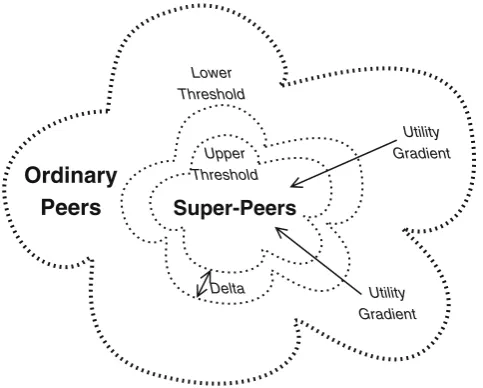
In a dynamic system, the super-peer election thresh-old constantly changes over time due to peer arrivals and departures, utility changes of individual peers, sta-tistical error in the approximation of system proper-ties, and system load variability. Hence, peers need to periodically recompute the threshold and their own utility in order to update the super-peer set. However, frequent switches between super-peers and ordinary peers increase the system overhead, for example due to data migration and synchronisation between super-peers. In order to avoid peers frequently switching roles between super-peer and ordinary peer, the system uses two separate thresholds for the super-peer election, an upper threshold, tu, and a lower threshold, tl, where
tu>tl(see Fig.3). An ordinary peer becomes a
super-peer when its utility rises above tu, while a peer stops to
be super-peer when its utility drops below tl. This way,
the system exhibits the property of hysteresis, as peers between the higher and lower utility thresholds do not switch their status, and the minimum utility change required for a peer to switch its status is =tu−tl.
Figure4shows the skeleton of the super-peer election algorithm.
2.5 Estimating system properties
Upper Threshold
Utility Gradient
Utility Gradient
Ordinary
Peers Super-Peers
Delta Lower Threshold
Fig. 3 Super-peer election with two utility thresholds on the gradient topology
required for the calculation of the super-peer election thresholds. The algorithm approximates the current number of peers in the system, N, the maximum peer utility in the system, Max, the average peer load in the system, L, a cumulative utility histogram, H, and a cumulative capacity histogram, Hc. Depending on
the super-peer election method, peers may only need a subset of these system properties.
The aggregation algorithm is based on periodic gos-sipping. Each peer p maintains its own estimates of N, Max, L, H, and Hc, denoted N
p, Maxp, Lp, Hp, and
Hcp, respectively, and stores a set,Tp, that contains the
currently executing aggregation instances.
Each peer runs an active and a passive thread, where the active thread initiates one gossip exchange per time step and the passive thread responds to all gossip requests received from neighbours. On average, a peer
whiletruedo 1
ifsuper-peerthen 2
threshold calculateLowerT hreshold() 3
ifU(p)<thresholdthen 4
becomeOrdinaryPeer() 5
end 6
end 7
else 8
threshold calculateU pperT hreshold() 9
ifU(p)>thresholdthen 10
becomeSuperPeer() 11
end 12
end 13
[image:8.595.50.292.53.247.2]end 14
Fig. 4 Super-peer election algorithm at peer p
sends and receives two aggregation messages per time step. When initiating a gossip exchange at each time step, peer p selects a random neighbour, q, and sends Tpto q. Peer q responds immediately by sendingTqto
p. Upon receiving their sets, both peers merge them us-ing an update()operation described later. The general structure of the algorithm is based on Jelasity’s push-pull epidemic aggregation [15].
The aggregation algorithm can be intuitively ex-plained using the concept of aggregation instances. An aggregation instance is a computation that generates a new approximation of N, Max, L, H, and Hc for all
peers in the system. Aggregation instances may overlap in time and each instance is associated with a unique identifier id. Potentially any peer can start a new ag-gregation instance by generating a new id and creating a new entry in Tp. As the new entry is propagated
throughout the system, other peers join the instance by creating corresponding entries with the same id. Thus, each entry stored by a peer corresponds to one aggregation instance that this peer is participating in. Eventually, the instance is propagated to all peers in the system. Every instance also has a finite time-to-live, and when an instance ends, all participating peers remove the corresponding entries and generate new approximations of N, Max, L,H, and Hc.
Formally, each entry, Tp, inTpof peer p is a tuple
consisting of eight values,
(id,ttl, w,m,l, λ,h,hc) (14)
where id is the unique aggregation instance identifier, ttl is the time-to-live for the instance, w is the weight of the tuple (used to estimate N), m is the current estimation of Max, l is the current estimation of L,λis the histogram width used in this aggregation instance, while h and hc are two B-dimensional vectors used in
the estimation of H and Hc, respectively.
At each time step, each peer p starts a new aggre-gation instance with probability Ps by creating a local
tuple
id,T T L,1,U(p),L(p), λ, Ip, Icp
(15)
where id is chosen randomly, T T L is a system constant, Ipis a utility histogram containing one peer p
Ip(i)=
0 i f U(p) <i·λ
1 i f U(p)≥i·λ (16) and Ic
pis a capacity histogram initialised by p
Icp(i)=
0 i f U(p) <i·λ
The bin widthλis set to Maxp
B , where B is the number
of bins in the histograms H and Hc. Probability Ps is
calculated as 1
Np·F, where F is a system constant that
regulates the frequency of peers’ starting aggregation instances. In a stable state, with a steady number of peers in the system, a new aggregation instance is cre-ated on average with frequency 1
F. Furthermore, since
an aggregation instance lasts T T L time steps, a peer participates on average in less than T T LF aggregation instances, and hence, stores less thanT T L
F tuples.
As the initial tuple is disseminated by gossipping, peers join the new aggregation instance. It can be shown that in push-pull epidemic protocols, the dis-semination speed is super-exponential, and with a very high probability, every peer in the system joins an aggregation instance within just several time steps [15]. The tuple merge procedure, update(Tp,Tq), consists
of the following steps. First, for each individual tuple Tq=(id,ttlq, wq,mq,lq, λq,hq,hcq)∈Tqreceived by
p from q, ifTpdoes not contain a local tuple identified
by id, and ttlq≥ T T L2 , peer p creates a local tuple
id,ttlq,0,U(p),L(p), λq, Ip, Icp
(18) and adds it toTp. This way, peer p joins a new
aggrega-tion instance id and introduces its own values of U(p), C(p),and L(p)to the computation. However, if ttlq<
T T L
2 , peer p should not join the aggregation, as there
is not enough time before the end of the aggregation instance to disseminate the information about p and to calculate accurate aggregates. This usually happens if p has just joined the P2P overlay and receives an aggregation message that belongs to an already running aggregation instance. In this case, the update operation is aborted by p.
In the next step, for each tuple Tq=(id,ttlq, wq,mq,
lq, λq,hq,hcq)∈Tq, peer p replaces its own tuple Tp= (id,ttlp, wp,mp,lp, λp,hp,hcp)∈Tpwith a new tuple
Tn=(id,ttln, wn,mn,ln, λn,hn,hcn)such that
ttln=
ttlp+ttlq
2 −1, wn=
wp+wq
2 , ln=
lp+lq
2
(19) mn=max(mp,mq), λn=λp=λq, and hn and hcn are
new histograms such that
hn(i)=
hp(i)+hq(i)
2 , h
c n(i)=
hc
p(i)+hcq(i)
2 (20)
for each i∈ {1, ...,B}. Thus, peer p merges its local tuples with the tuples received from q, contributing to the aggregate calculation.
Finally, for each tuple Tp=(id, ttlp, wp, mp, lp, λp, hp, hcp)∈Tp, such that ttlp≤0, peer p removes
Tp fromTp and updates the current estimates in the
following way: Np= w1p, Maxp=mp, Lp=lp,λ=λp,
and for each i∈ {1, ...,B}
Hp(i)=
hp(i) wp ,
Hcp(i)=h
c p(i) wp .
(21)
The algorithm has the following invariant. For each aggregation instance id, the weights of all tuples in the system associated with id sum up to1, with 1
westimating
the number of peers participating in this aggregation instance.
Peers joining the P2P overlay obtain the current values of N, Max, L, H, and Hc from one of their
initial neighbours. Peers leaving, if they do not crash, perform a leave procedure that reduces the aggregation error caused by peer departures, where they send all currently stored tuples to a randomly chosen neigh-bour. The receiving neighbour adds the weights of the received tuples to its own tuples in order to preserve the weight invariant. Similarly as when joining an aggrega-tion instance, peers do not perform the leave procedure for tuples with the time-to-live value below T T L2 , as there is not enough time left in the aggregation instance to propagate the weight from these tuples between peers and to obtain accurate aggregation results.
It can be shown, as in [15], that the values Np, Maxp,
Lp,Hp, and Hcpgenerated by the algorithm at the end
of an aggregation instance at each peer p approximate the true system properties N, Max, L,H, and Hc, with
the average error, or variance, decreasing exponentially with T T L.
In order to calculate the super-peer election thresh-olds, peers need to complete two aggregation instances, which requires2·T T L time steps. In the first instance, peers estimate the maximum peer utility (Max) and determine the histogram bin width (λ= Max
B ). In the
following instance, peers generate utility histograms (H or Hc), estimate the system size (N) and load
(L), and calculate appropriate thresholds, as defined in Section2.4.
2.6 Discovering high utility peers
The gradient structure of the topology allows an effi-cient search heuristic, called gradient search, that en-ables the discovery of high utility peers in the system. Gradient search is a multi-hop message passing algo-rithm, that routes messages from potentially any peer in the system to high utility peers in the core, i.e., peers with utility above the super-peer election threshold.
neighbour, i.e., to a neighbour q whose utility is equal to
max
x∈Sp∪Rp
Up(x)
. (22)
Thus, messages are forwarded along the utility gradi-ent, as in hill climbing and similar techniques.
Local maxima should not occur in an idealised gra-dient topology, however, every P2P system is under constant churn and the gradient topology may undergo local perturbations from the idealised structure. In or-der to prevent message looping in the presence of such local maxima, a list of visited peers is appended to each search message, and a constraint is imposed that forbids message forwarding to previously visited peers.
The algorithm exploits the information contained in the topology for routing messages and achieves a significantly better performance than general-purpose search techniques for unstructured P2P networks, such as flooding or random walking, that require the com-munication with a large number of peers in the system [16]. Gradient search also reduces message loss rate by preferentially forwarding messages to high utility, and hence more stable, peers.
However, greedy message routing to the highest utility neighbours has the drawback that messages are always forwarded along the same paths, unless the topology changes, which may lead to a significant im-balance between high utility peers in the core. This is especially probable in the presence of “heavy hitters”, i.e., peers generating large amounts of traffic, as com-monly seen in P2P systems [4]. Load balancing can be improved in the gradient topology by randomising the routing, for example, if a peer, p, selects the next-hop destination, q, for a message with probability, Pp(q),
given by the Boltzmann exploration formula [17]
Pp(q)=
e(Up(q)/Temp)
i∈Sp∪Rpe(
Up(i)/Temp)
(23)
where Temp is a parameter of the algorithm called the temperature that determines the “greediness” of the algorithm. Setting Temp close to zero causes the algorithm to be more greedy and deterministic, as in gradient search, while if Temp grows to infinity, all neighbours are selected with equal probability as in ran-dom walking. Thus, the temperature enables a trade-off between exploitative (and deterministic) routing of messages towards the core, and random exploration that spreads the load more equally between peers. The impact of the temperature on the performance of Boltzmann search has been studied in [16].
2.7 Supporting the decentralised registry service
The registry stores information about services available in the system. For each registered service, it stores a record that consists of the service address, text descrip-tion, interface, attributes, etc. The registry allows each peer to register a new service, update a service record, delete a record, and search for records that satisfy certain criteria. Each record can be updated or deleted only by its owner, that is the peer that created it.
For fault-tolerance and performance reasons, the registry service is replicated between a limited number of high-utility super-peers. Each peer periodically runs the aggregation algorithm, calculates the super-peer election thresholds, and potentially become a super-peer if needed.
It is assumed that the average size of a service record is relatively small (order of kilobytes), and hence, each super-peer has enough storage space to host a full registry replica, i.e., a copy of all service records. Due to this replication scheme, every super-peer can independently handle any search query without com-municating with other super-peers. This is important, since complex search, for example based on attributes, keywords, or range queries, is known to be expensive in distributed systems [9,18]. It is also assumed that search operations are significantly more frequent than update operations, and hence, the registry is optimised for handling search.
In order to perform a search on the registry, a peer generates a query and routes it using gradient search to the closest super-peer. If the super-peer is heavily-loaded, it may forward the query to another super-peer which has enough capacity to handle it. The super-peer processes the query and returns the search results directly to the originating peer. Optionally, clients may cache super-peer addresses and contact super-peers directly in order to reduce the routing over-head.
Conflicts between concurrent updates are resolved based on the update timestamps. Every record can be updated only by its owner, and it is assumed that the owner is responsible for assigning consistent timestamps for its own update operations. Moreover, super-peers do not need to maintain a membership list of all replicas in the system. Due to the properties of the gradient topology, all super-peers are located within a connected component, and hence, every super-peer eventually receives every update.
Super-peers are elected using a load-based utility threshold. Each peer defines its capacity as the maxi-mum number of queries it can handle at one time. The load at a peer is defined as the number of queries the peer is currently processing. The super-peer election threshold is calculated in such a way that the super-peers have sufficient capacity to handle all queries is-sued in the system. When the load in the system grows, new replicas are automatically created.
2.8 Supporting additional SOA facilities
Apart from the service registry, which needs to be present in a service-oriented architecture, many SOAs rely on other infrastructural facilities, such as business transaction services, or ranking systems, that are of-ten implemented in a centralised fashion. This section shows an approach to decentralise such facilities using the gradient topology.
Assuming two applications, A and B, where each application has different peer utility requirements that can be encapsulated in two utility functions, UA and
UB, respectively, each application defines its utility
threshold, tA and tB, and the goal of the system is
to elect and exploit super-peers p such that either UA(p) >tAor UB(p) >tB.
A naive approach is to generate two independent gradient overlays, using the two utility functions and the algorithms described in the previous sections. How-ever, this would double the system overhead. A better approach is to combine the two utility functions into one general utility function U and to generate one gradient overlay shared by both applications. A conve-nient way of defining such a common utility function is U(p)=maxUA(p),UB(p)
. (24)
This has the advantage that both, peers with high value of UAand peers with high value of UB, have high utility
U , and hence are located in the core and can be discov-ered using gradient search. The only change required in the routing algorithm is that a search message, once delivered to a high utility peer p in the core, may have to be forwarded to a different peer in the core, since
p either has a high value UA or UB. This last step,
however, with a high probability can be achieved in one hop, since peers in the core are well-connected.
The super-peer election thresholds, tA and tB, are
estimated using the same aggregation algorithm, where the histograms for both UA and UB are generated
through the same aggregation instance in order to reduce the algorithm overhead. However, a potential problem may appear if the two utility functions, UAand
UB, have significantly different value ranges, since the
composed utility U may be dominated by one of the utility functions. For example, if UAhas values within
range[0..1]and UBhas values in range[1..100], then U
is essentially equal to UB, and searching for peers with
high UAbecomes inefficient.
One way to mitigate this problem is to define the two utility functions in such a way that both have the same value ranges, e.g., [0..1]. However, this requires system-wide knowledge about peers. Simple transformations or projections onto a fixed interval, for example using a sigmoid function, do not fix the problem, since if one function has higher values than the other function, the same relation holds when the transformation has been applied. A better approach is to scale one of the two utility functions using the current values of the super-peer election thresholds, for example in the following way
U(p)=max UA(p),
tA
tB
UB(p)
. (25)
This has the advantage that the core of the gradient topology, determined by the threshold tA, contains
peers with UA above tA and peers with UB above tB,
since if U(p) >tAfor a peer p then either UA(p) >tA
or UB(p) >tB.
Similarly, in the general case, where a gradient topol-ogy supports more than two applications, all utility functions are scaled by their respective thresholds
U(p)=max UA(p),
tA
tB
UB(p),
tA
tC
UC(p), . . .
.
(26)
This way, all peers required by the higher-level ap-plications (i.e., each peer p such that UA(p) >tA or
UB(p) >tBor UC(p) >tC and so on) have utility U(p)
above tA, and can be elected super-peers using the
single utility threshold tA.
Gradient Search Gradient
Search
Ordinary Peers
Replica Placement Threshold Application A Super-Peers
Application B Super-Peers X
[image:12.595.51.289.52.267.2]Z Y
Fig. 5 Super-peer election and discovery in a gradient topology supporting two different applications A and B
peers perform gradient search to discover application B peers. Peers X and Y locate an “ A-type” super-peer in the core and their request is forwarded to a “B-type” peer. Peer Z discovers a “B-“B-type” super-peer directly.
2.9 Peer bootstrap
Bootstrap is a process in which a peer obtains an ini-tial configuration in order to join the system. In P2P systems, this primarily involves obtaining addresses of initial neighbours. Once a peer connects to at least one neighbour, it can receive from this neighbour the addresses of other peers in the system as well as other initialisation data, such as the current values of aggre-gates.
However, initial neighbour discovery is challenging in wide-area networks, such as the Internet, since a broadcast facility is not widely available. In particu-lar, the IP multicast protocol has not been commonly adopted by Internet service providers due to design and deployment difficulties [20]. Most existing P2P systems rely on centralised bootstrap servers that maintain lists of peer addresses.
This section describes a bootstrap procedure that consists of two stages. In the first stage, a peer attempts to obtain initial neighbour addresses from a local cache saved during the previous session, for example on a local disk. This can be very effective; Stutzbach et al. [7] analyse statistical properties of peer session times in a number of deployed P2P systems and show that
if a peer caches the addresses of several high-uptime neighbours, there is a high probability that some of these high-uptime neighbours will be on-line during the peer’s subsequent session. Furthermore, such a bootstrap strategy is fully decentralised, as it does not require any fixed infrastructure, and it scales with the system size.
However, if all addresses in the cache are unavailable or the cache is empty, for example if the peer is joining the system for the first time, the peer needs to have an alternative bootstrap mechanism. In the second stage, peers obtain initial neighbour addresses from a boot-strap node. The IP addresses of the bootboot-strap nodes are either hard-coded in the application, or preferably, are obtained by resolving well known domain names. This latter approach allows greater flexibility, as bootstrap nodes can be added or removed over the course of the system’s lifetime. Moreover, the domain name may resolve to a number of bootstrap node addresses, for example selected using a round-robin strategy, in order to balance the load between bootstrap nodes.
Each bootstrap node is independent and maintains its own cache containing peer addresses. The cache size and the update strategy are critical in a P2P system, as the bootstrap process may have a strong impact on the system topology, particularly in the case of high churn rates. If the cache is too small, subsequently joining peers have similar initial neighbours, and in consequence, the system topology may become highly clustered or even disconnected. On the other hand, a large cache is more difficult to keep up to date and may contain addresses of peers that have already left the system.
A simple cache update strategy is to add the ad-dresses of currently bootstrapped peers and to remove addresses in a FIFO order. However, this strategy has the drawback that it generates a topology where join-ing peers are highly connected with each other, which again leads to a highly-clustered topology and sys-tem partitioning. A better approach is to continuously “crawl” the P2P network and “harvest” available peer addresses. In this case, the bootstrap node periodically selects a random peer from the cache, obtains the peer’s current neighbours, adds their addresses to the cache, and removes the oldest entries in the cache. This has the advantage that the addresses stored in the cache are close to a random sample from all peers in the system.
3 Evaluation
since P2P systems usually exhibit complex, dynamic behaviour that is difficult to predict a priori. Theoret-ical system analysis is difficult, and often infeasible in practice, due to the system complexity. At the same time, a full implementation and deployment of a P2P system on a realistic scale requires extremely large amounts of resources, such as machines and users, that are prohibitive in most circumstances. Consequently, the approach followed in this paper is simulation.
However, designing P2P simulations is also challeng-ing. The designer has to decide upon numerous system assumptions and parameters, where the appropriate choices or parameter values are non-trivial to deter-mine. Furthermore, dependencies between different elements of a complex system are often non-linear, and a relatively small change of one parameter may result in a dramatic change in the system behaviour.
Moreover, due to the large scale and complexity, P2P systems are not amenable to visualisation techniques, as a display millions of peers, connections, and mes-sages is not human-readable. P2P simulations must con-tinuously collect and aggregate statistical information about the system in order to, detect topology partitions, identify bottlenecks, measure global system properties, etc. Such frequent and extensive measurements are often computationally expensive, which adds further challenges to analysing P2P systems.
3.1 Evaluation goals
In order to evaluate the gradient topology and its usage in the SOA, the behaviour of the three main algorithms are studied: the neighbour selection algorithm, super-peer election (i.e., registry replica placement), and re-quest routing.
The neighbour selection algorithm is evaluated through an analysis of the generated topology, where the analysed properties include the average peer de-gree (i.e., number of neighbours), clustering coefficient, average path length in the topology, and the average percentage of globally optimal neighbours in a peer’s neighbourhood set. The super-peer election algorithm, and indirectly the aggregation algorithm, are evaluated in a simulation run by measuring the average differ-ence between the desired and the observed numbers of super-peers in the system, the average number of switches between super-peers and ordinary peers, and the total capacity, utilisation and load of super-peers. Finally, the performance of the routing algorithms on the gradient topology is studied by measuring the av-erage request hop count and avav-erage failure rate (i.e., percentage of request messages that are lost) in a simu-lation run.
The algorithms are run in a number of different experiments that examine the impact of relevant system parameters on the system performance, such as the number of peers, churn rate, average load, and super-peer thresholds. The evaluation shows that the gradi-ent topology scales to a large number of peers and is resilient to high peer churn rates.
For the interested reader, a further, more compre-hensive evaluation of the gradient topology can be found in [21]. In particular, [21] compares a number of state-of-the-art super-peer election techniques, and shows that the aggregation-based election used in this paper generates higher-quality super-peer sets, accord-ing to a number of different metrics, at a similar cost, compared to the other known super-peer election algo-rithms.
3.2 System model
The gradient topology has been evaluated in a discrete event simulator. The system consists of a set of peers, connections between peers, and messages passed be-tween peers. It is assumed that all peers are mutually reachable and any pair of peers can potentially establish a connection. The neighbourhood model is symmetric, as discussed earlier in Section2.3. The maximum num-ber of neighbours for a peer at any given time is limited to 26, however, as shown later, peers rarely approach this limit, as the desired number of peer neighbours is set to13(7for the random set and6for the similar set). The P2P network is under constant churn, with peer session times determined probabilistically, following a Pareto distribution. While the paper describes a peer leave procedure, it is hard to estimate how many peers in a real-world system would perform the procedure when leaving. For that reason, the worst case scenario is assumed in the experiments, where no peers perform the leave procedure. Joining peers are bootstrapped by a centralised server, which provides addresses of initial neighbours. The server obtains these addresses by “crawling” the P2P network and maintaining a FIFO buffer with 1,000 entries. The bootstrap server is also used for initiating aggregation instances.
experiments in this paper is set to10 min. Assuming a time step of 6seconds, this corresponds to a mean session time of100time steps and a churn rate of0.7% peers per time step (0.11% peers per second).
While session time distributions are highly-skewed in existing P2P systems, there is no general consensus whether these distributions are heavy-tailed and which mathematical model best fits the empirically observed peer session times. Sen and Wong [4] observe a heavy-tailed distribution of the peer session time, however, Chu et al. [22] suggest a log-quadratic peer session time distribution, while Stutzbach and Rejaie [7] suggest the Weibull distribution. Moreover, Stutzbach and Rejaie discovered that the best power-law fit for the peer session times in a number of BitTorrent overlays has an exponent whose value is between2.1and2.7, and therefore the distributions are not heavy-tailed. In the experiments in this paper, the peer session times are set according to the Pareto distribution with a median of
10min and exponent2.0(which is border case between heavy-tailed and non-heavy-tailed distributions).
3.3 Service registry simulation
The service registry is maintained by super-peers elected using the adaptive thresholds. The capacity value C(p) determines the maximum number of re-quests a peer p can simultaneously handle if elected super-peer and hosting a registry replica. The load at peer p, denoted L(p), is defined as the number of requests currently being processed at peer p. The capacity values are assigned to peers according to the Pareto distribution with exponent of 2 and average value of1, which models peer resource heterogeneity in the system. Moreover, peer utility is defined as U(p)=C(p)·logU p(p) (27) where the capacity is weighted by the peer’s current uptime in order to promote stable peers. As discussed in Section2.2, this utility metric is fully predictable.
At every step, each peer p in the system emits a search request with probability Preq(p). Probability
Preq(p)follows the Pareto distribution between peers
with exponent2and average value Preq=0.01. Peers
that generate more traffic correspond to the so called “heavy hitters” in the P2P system.
Request routing is performed in two stages. First, a newly generated request is routed using Boltzmann search with low temperature T=0.5steeply to the core until it is delivered to a super-peer. In the second stage, the request is forwarded between super-peers in the core until it is delivered to super-peer s that has enough free capacity to handle the request (i.e., C(s)−L(s)≥
1). Once super-peer s accepts the requests and starts handling it, its load is increased by one. When the request processing finishes, the load at the super-peer is reduced by one.
Forwarding between super-peers is probabilistic. A super-peer p forwards the request to one of its neigh-bours, q, such that Up(q) >t, where t is the current
super-peer election threshold, with probability Pp(q) proportional to q’s capacity
Pp(q)= C(q)
Up(x)>tC(x)
. (28)
The bias towards high capacity neighbours improves the load balancing property of the routing algorithm. If no neighbour q exists such that Up(q) >t, the
re-quest is routed randomly. Every rere-quest has a time-to-live value, initialised to T T Lreq=30, and decremented
each time a request is forwarded between peers. Thus, a request message can be lost when its time-to-live value drops to zero or when the peer that is currently transmitting it leaves the system.
3.4 Maintenance cost
At every time step, each peer executes the neighbour selection, aggregation, super-peer election, and mes-sage routing algorithms. A peer sends on average 4
neighbour selection messages per time step (a request and response for Sp and similarly a request and
re-sponse for Rp) and less than4aggregation messages per
time step (2request messages and2response messages, since for F=25 and T T L=50 a peer participates on average in less than 2 aggregation instances, as explained in Section2.5). The election algorithm does not generate any messages. It can be shown that the size of both the neighbour selection and aggregation messages is below 1KB, and therefore, for the basic topology maintenance, a peer sends less than 8KB of data per time step. Given a time step of 6 seconds, this corresponds to an average traffic rate of1.25KB/s. Moreover, this cost is independent of the system size and the churn rate, since the aggregation and neighbour selection algorithms are executed at a fixed periodicity and always generate the same number of messages per time step. However, the cost associated with gradient search depends on the rate of requests and the size of request messages, and hence is application-specific.
3.5 Topology structure
experiment begins with a network consisting of a single peer, and the network size is increased exponentially by adding a fixed percentage of peers at each time step until the size grows to100,000peers. At the following time steps, the system is under continuous peer churn, however, the rate of arrivals is equal to the rate of departures and the system size remains constant.
The following notation and metrics are used. The system topology T is a graph(V,E), where V is the set of peers in the system, and E is the set of edges between peers determined by the neighbourhood sets:(p,q)∈ E if q∈ Sp∪Rp. The graph is undirected, since the
neighbourhood relation is symmetric and if q∈Sp∪
Rp then p∈Sq∪Rq. Similarly, sub-topologies TS= (V,ES) and TR=(V,ER) are defined based on the
similarity and random neighbourhood sets, Spand Rp,
accordingly, where (p,q)∈ES if q∈Sp, and(p,q)∈
ERif q∈ Rp.
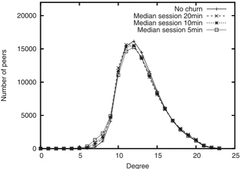
Figure6shows the average peer degree distribution in four systems with100,000peers and different churn rates, where each plotted point represents the total number of peers in the system with a given neighbour-hood size. The graph has been obtained by running four experiments with different churn rates, each for
2,000time steps, generating peer degree distributions every40 time steps, and averaging the sample sets at the end of each experiment in order to reduce the statistical noise. The same procedure has been applied to generate all the remaining graphs in this subsection.
The obtained degree distributions resemble a normal distribution, where majority of peers have approxi-mately13neighbours, as desired. Moreover, the distrib-utions are nearly identical for all churn rates, suggesting good resilience of the neighbour selection algorithm to peer churn.
0 5000 10000 15000 20000
0 5 10 15 20 25
Number of peers
Degree
[image:15.595.51.290.521.688.2]No churn Median session 20min Median session 10min Median session 5min
Fig. 6 Peer degree distribution in four systems with different churn rates
Vris defined as a subset of peers in the system, Vr ⊂
V, that contains r highest utility peers. Formally,
Vr =
p∈V|U(p)≥U(pr)
(29) where pr is the rth highest utility peer in the system.
In order to investigate the correlation between peer degree and peer utility, the average peer degree is calculated for a number of Vr sets in T, TS and TR.
Figure7shows the results of this experiment. The plots are nearly flat, indicating that the average number of neighbours is independent from the peer utility, and in particular, the highest utility peers are not overloaded by excessive connections from lower utility peers. The slight increase in the degree of the 12 highest utility peers is caused by the fact that these peers cannot find any higher utility neighbours, and hence, connect to lower utility peers, generating a locally higher average degree.
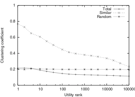
Similarly, Fig. 8 shows the clustering coefficient in topologies T, TS and TRfor a number of Vr set with
increasing utility rank r. In the TStopology, the
coeffi-cient gradually grows as peer utility increases, almost reaching the value of 0.8 for r=1, which indicates that the highest utility peers in the system are highly connected with each other and constitute a “core” in the network. At the same time, the coefficient is nearly constant in TR, since the preference function for the
random sets is independent of peer utility.
Given global knowledge about the system in a P2P simulator, the optimal neighbourhood set S∗p for each peer p can be determined using the neighbour pref-erence function defined by formulas (2) and (3) in Section 2.3. Formally, S∗p is a subset of all peers in the system, S∗p⊂V, such that min(S∗p)≥max(V\S∗p), where the≥relation is defined in formulas (2) and (3).
0 5 10 15 20
1 10 100 1000 10000 100000
Average degree
Utility rank
[image:15.595.308.541.524.688.2]Total Similar Random