Automatic Text Scoring Using Neural Networks

Automatic Text Scoring Using Neural Networks

Dimitrios Alikaniotis Department of Theoretical

and Applied Linguistics University of Cambridge

Cambridge, UK [email protected]

Helen Yannakoudakis The ALTA Institute Computer Laboratory University of Cambridge

Cambridge, UK [email protected]

Marek Rei The ALTA Institute Computer Laboratory University of Cambridge

Cambridge, UK [email protected]

Abstract

Automated Text Scoring (ATS) provides a cost-effective and consistent alternative to human marking. However, in order to achieve good performance, the pre-dictive features of the system need to be manually engineered by human ex-perts. We introduce a model that forms word representations by learning the ex-tent to which specific words contribute to the text’s score. Using Long-Short Term Memory networks to represent the mean-ing of texts, we demonstrate that a fully automated framework is able to achieve excellent results over similar approaches. In an attempt to make our results more interpretable, and inspired by recent ad-vances in visualizing neural networks, we introduce a novel method for identifying the regions of the text that the model has found more discriminative.

1 Introduction

Automated Text Scoring (ATS) refers to the set of statistical and natural language processing tech-niques used to automatically score a text on a marking scale. The advantages of ATS systems have been established since Project Essay Grade (PEG) (Page, 1967; Page, 1968), one of the earli-est systems whose development was largely moti-vated by the prospect of reducing labour-intensive marking activities. In addition to providing a cost-effective and efficient approach to large-scale grading of (extended) text, such systems ensure a consistent application of marking criteria, there-fore facilitating equity in scoring.

There is a large body of literature with re-gards to ATS systems of text produced by non-native English-language learners (Page, 1968;

At-tali and Burstein, 2006; Rudner and Liang, 2002; Elliot, 2003; Landauer et al., 2003; Briscoe et al., 2010; Yannakoudakis et al., 2011; Sakaguchi et al., 2015, among others), overviews of which can be found in various studies (Williamson, 2009; Dikli, 2006; Shermis and Hammer, 2012). Im-plicitly or exIm-plicitly, previous work has primarily treated text scoring as a supervised text classifica-tion task, and has utilized a large selecclassifica-tion of tech-niques, ranging from the use of syntactic parsers, via vectorial semantics combined with dimension-ality reduction, to generative and discriminative machine learning.

As multiple factors influence the quality of texts, ATS systems typically exploit a large range of textual features that correspond to different properties of text, such as grammar, vocabulary, style, topic relevance, and discourse coherence and cohesion. In addition to lexical and part-of-speech (POS) ngrams, linguistically deeper fea-tures such as types of syntactic constructions, grammatical relations and measures of sentence complexity are among some of the properties that form an ATS system’s internal marking criteria. The final representation of a text typically consists of a vector of features that have been manually se-lected and tuned to predict a score on a marking scale.

Although current approaches to scoring, such as regression and ranking, have been shown to achieve performance that is indistinguishable from that of human examiners, there is substantial man-ual effort involved in reaching these results on dif-ferent domains, genres, prompts and so forth. Lin-guistic features intended to capture the aspects of writing to be assessed are hand-selected and tuned for specific domains. In order to perform well on different data, separate models with distinct fea-ture sets are typically tuned.

Prompted by recent advances in deep learning and the ability of such systems to surpass state-of-the-art models in similar areas (Tang, 2015; Tai et al., 2015), we propose the use of recurrent neural network models for ATS. Multi-layer neural net-works are known for automatically learning use-ful features from data, with lower layers ing basic feature detectors and upper levels learn-ing more high-level abstract features (Lee et al., 2009). Additionally, recurrent neural networks are well-suited for modeling the compositionality of language and have been shown to perform very well on the task of language modeling (Mikolov et al., 2011; Chelba et al., 2013). We therefore propose to apply these network structures to the task of scoring, in order to both improve the per-formance of ATS systems and learn the required feature representations for each dataset automat-ically, without the need for manual tuning. More specifically, we focus on predicting a holistic score for extended-response writing items.1

However, automated models are not a panacea, and their deployment depends largely on the abil-ity to examine their characteristics, whether they measure what is intended to be measured, and whether their internal marking criteria can be in-terpreted in a meaningful and useful way. The deep architecture of neural network models, how-ever, makes it rather difficult to identify and ex-tract those properties of text that the network has identified as discriminative. Therefore, we also describe a preliminary method for visualizing the information the model is exploiting when assign-ing a specific score to an input text.

2 Related Work

In this section, we describe a number of the more influential and/or recent approaches in automated text scoring of non-native English-learner writing. Project Essay Grade (Page, 1967; Page, 1968; Page, 2003) is one of the earliest automated scor-ing systems, predictscor-ing a score usscor-ing linear regres-sion over vectors of textual features considered to be proxies of writing quality. Intelligent Essay Assessor (Landauer et al., 2003) uses Latent Se-mantic Analysis to compute the seSe-mantic similar-ity between texts at specific grade points and a test text, which is assigned a score based on the ones in 1_{The task is also referred to as Automated Essay Scoring.}

Throughout this paper, we use the termstextandessay (scor-ing) interchangeably.

the training set to which it is most similar. Lons-dale and Strong-Krause (2003) use the Link Gram-mar parser (Sleator and Templerley, 1995) to anal-yse and score texts based on the average sentence-level scores calculated from the parser’s cost vec-tor.

The Bayesian Essay Test Scoring sYstem (Rud-ner and Liang, 2002) investigates multinomial and Bernoulli Naive Bayes models to classify texts based on shallow content and style features. e-Rater (Attali and Burstein, 2006), developed by the Educational Testing Service, was one of the first systems to be deployed for operational scor-ing in high-stakes assessments. The model uses a number of different features, including aspects of grammar, vocabulary and style (among others), whose weights are fitted to a marking scheme by regression.

Chen et al. (2010) use a voting algorithm and address text scoring within a weakly supervised bag-of-words framework. Yannakoudakis et al. (2011) extract deep linguistic features and employ a discriminative learning-to-rank model that out-performs regression.

Recently, McNamara et al. (2015) used a hier-achical classification approach to scoring, utilizing linguistic, semantic and rhetorical features, among others. Farra et al. (2015) utilize variants of lo-gistic and linear regression and develop models that score persuasive essays based on features ex-tracted from opinion expressions and topical ele-ments.

There have also been attempts to incorporate more diverse features to text scoring models. Kle-banov and Flor (2013) demonstrate that essay scoring performance is improved by adding to the model information about percentages of highly associated, mildly associated and dis-associated pairs of words that co-exist in a given text. So-masundaran et al. (2014) exploit lexical chains and their interaction with discourse elements for evalu-ating the quality of persuasive essays with respect to discourse coherence. Crossley et al. (2015) identify student attributes, such as standardized test scores, as predictive of writing success and use them in conjunction with textual features to develop essay scoring models.

In 2012, Kaggle,2 _{sponsored by the Hewlett} Foundation, hosted the Automated Student As-sessment Prize (ASAP) contest, aiming to

strate the capabilities of automated text scoring systems (Shermis, 2015). The dataset released consists of around twenty thousand texts (60%of which are marked), produced by middle-school English-speaking students, which we use as part of our experiments to develop our models.

3 Models

3.1 C&W Embeddings

Collobert and Weston (2008) and Collobert et al. (2011) introduce a neural network architecture (Fig. 1a) that learns a distributed representation for each wordwin a corpus based on its local context. Concretely, suppose we want to learn a represen-tation for some target wordwtfound in ann-sized

sequence of words S = (w1, . . . , wt, . . . , wn)

based on the other words which exist in the same sequence(∀wi ∈ S |wi 6=wt). In order to derive

this representation, the model learns to discrimi-nate betweenS and some ‘noisy’ counterpart S0

in which the target wordwt has been substituted

for a randomly sampled word from the vocabu-lary:S0 _{= (w}

1, . . . , wc, . . . , wn|wc∼ V). In this

way, every wordwis more predictive of its local context than any other random word in the corpus. Every word in V is mapped to a real-valued vector in Ω via a mapping function C(·) such that C(wi) = hM?ii, where M ∈ RD×|V| is

the embedding matrix and hM?ii is the ith

col-umn of M. The network takes S as input by concatenating the vectors of the words found in it; st = hC(w1)|k. . .kC(wt)|k. . .kC(wn)|i ∈

RnD_{. Similarly, S}0 _{is formed by substituting} C(wt)forC(wc)∼M|wc6=wt.

The input vector is then passed through a hardtanhlayer defined as,

htanh(x) =

    

−1 x <−1

x −16x61

1 x >1

(1)

which feeds a single linear unit in the output layer. The function that is computed by the network is ultimately given by (4):

st=hM|?1k. . .kM|?tk. . .kM|?ni| (2)

i=σ(Whist+bh) (3)

f(st) =Wohi+bo (4)

f(s),bo∈R1 Woh ∈RH×1

Whi∈RD×H s∈RD bo∈RH

whereM,Woh,Whi,bo,bhare learnable

param-eters, D, H are hyperparameters controlling the size of the input and the hidden layer, respectively;

σis the application of an element-wise non-linear function (htanhin this case).

The model learns word embeddings by ranking the activation of the true sequenceS higher than the activation of its ‘noisy’ counterpart S0_{. The}

objective of the model then becomes to minimize the hinge loss which ensures that the activations of the original and ‘noisy’ ngrams will differ by at least 1:

losscontext(target, corrupt) =

[1−f(st) +f(sck)]+, ∀k∈ZE (5)

whereEis another hyperparameter controlling the number of ‘noisy’ sequences we give along with the correct sequence (Mikolov et al., 2013; Gut-mann and Hyv¨arinen, 2012).

3.2 Augmented C&W model

Following Tang (2015), we extend the previous model to capture not only the local linguistic en-vironment of each word, but also how each word contributes to the overall score of the essay. The aim here is to construct representations which, along with the linguistic information given by the linear order of the words in each sentence, are able to capture usage information. Words such asis,

are, to, at which appear with any essay score are

considered to be under-informative in the sense that they will activate equally both on high and low scoring essays. Informative words, on the other hand, are the ones which would have an impact on the essay score (e.g., spelling mistakes).

In order to capture those score-specific word

embeddings (SSWEs), we extend (4) by adding a

. . . . the recent advances

(a)

. . . . the recent advances

(b)

Figure 1: Architecture of the original C&W model (left) and of our extended version (right).

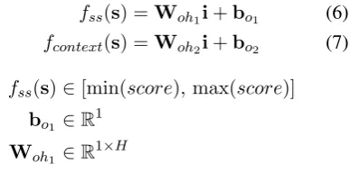
fss(s) =Woh1i+bo1 (6) fcontext(s) =Woh2i+bo2 (7)

fss(s)∈[min(score),max(score)] bo1 ∈R1

Woh1 ∈R1×H

The error we minimize forfss(wheressstands for

score specific) is themean squared errorbetween

the predictedyˆand the actual essay scorey:

lossscore(s) = _N1 N

X

i=1

(ˆyi−yi)2 (8)

From (5) and (8) we compute the overall loss function as a weighted linear combination of the two loss functions (9), back-propagating the error gradients to the embedding matrixM:

lossoverall(s) = α·losscontext(s,s

0₎

+ (1−α)·lossscore(s) (9)

whereα is the hyper-parameter determining how the two error functions should be weighted.α val-ues closer to0will place more weight on the score-specific aspect of the embeddings, whereas values closer to1will favour the contextual information. Fig. 2 shows the advantage of using SSWEs in the present setting. Based solely on the informa-tion provided by the linguistic environment, words such ascomputerandlaptopare going to be placed together with their mis-spelled counterparts

cop-muter and labtop(Fig. 2a). This, however, does

not reflect the fact that the mis-spelled words tend to appear in lower scoring essays. UsingSSWEs, the correctly spelled words are pulled apart in the

vector space from the incorrectly spelled ones, re-taining, however, the information thatlabtopand

copmuterare still contextually related (Fig. 2b).

3.3 Long-Short Term Memory Network

We use the SSWEs obtained by our model to derive continuous representations for each essay. We treat each essay as a sequence of tokens and explore the use of uni- and bi-directional (Graves, 2012) Long-Short Term Memory net-works (LSTMs) (Hochreiter and Schmidhuber, 1997) in order to embed these sequences in a vec-tor of fixed size. Both uni- and bi-directional LSTMs have been effectively used for embedding long sequences (Hermann et al., 2015). LSTMs are a kind of recurrent neural network (RNN) ar-chitecture in which the output at timetis condi-tioned on the input s both at time t and at time

t−1:

yt=Wyhht+by (10)

ht=H(Whsst+Whhht−1+bh) (11)

where st is the input at time t, and His usually

an element-wise application of a non-linear func-tion. In LSTMs,His substituted for a composite function defininghtas:

it= σ(Wisst_W+Wihht−1+

icct−1+bi) (12)

ft= σ(Wfsst_W+Wfhht−1+

fcct−1+bf) (13)

1 2 3 4 1

2 3

COPMUTAR COMPUTER

LAPTOP LABTOP

(a)

Standard neural embeddings

1 2 3 4

1 2 3

COPMUTAR COMPUTER

LAPTOP

LABTOP

(b)

Score-specific word embeddings

Figure 2: Comparison between standard and score-specific word embeddings. By virtue of appearing in similar environments, standard neural embeddings will place the correct and the incorrect spelling closer in the vector space. However, since the mistakes are found in lower scoring essays,SSWEs are able to discriminate between the correct and the incorrect versions without loss in contextual meaning.

the wthe

the wthe

recent wrecent

recent wrecent

advances wadvances

advances wadvances

. . . w...

. . . w...

− →

h

←−

h

y

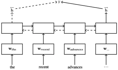
Figure 3: A single-layer Long Short Term Mem-ory(LSTM) network. The word vectorswi enter

the input layer one at a time. The hidden layer that has been formed at the last timestep is used to predict the essay score using linear regression. We also explore the use of bi-directional LSTMs (dashed arrows). For ‘deeper’ representations, we can stack more LSTM layers after the hidden layer shown here.

ot= σ(Wosst_W+Wohht−1+

occt+bo) (15)

ht=oth(ct) (16)

where g, σ and h are element-wise non-linear functions such as thelogistic sigmoid( 1

1+e−x) and

thehyperbolic tangent(e_e22zz−₊₁1);is the Hadamard

product;W,b are the learned weights and biases respectively; andi,f,oandcare the input, forget, output gates and the cell activation vectors respec-tively.

Training the LSTM in a uni-directional manner (i.e., from left to right) might leave out important information about the sentence. For example, our

interpretation of a word at some pointtimight be

different once we know the word atti+5. An

ef-fective way to get around this issue has been to train the LSTM in a bidirectional manner. This re-quires doing both a forward and a backward pass of the sequence (i.e., feeding the words from left to right and from right to left). The hidden layer element in (10) can therefore be re-written as the concatenation of the forward and backward hidden vectors:

yt=Wyh

←−_h| t

− →_h|

t

!

+by (17)

We feed the embedding of each word found in each essay to the LSTM one at a time, zero-padding shorter sequences. We form D -dimensional essay embeddings by taking the ac-tivation of the LSTM layer at the timestep where the last word of the essay was presented to the net-work. In the case of bi-directional LSTMs, the two independent passes of the essay (from left to right and from right to left) are concatenated together to predict the essay score. These essay embeddings are then fed to a linear unit in the output layer which predicts the essay score (Fig. 3). We use the

mean square errorbetween the predicted and the

gold score as our loss function, and optimize with RMSprop (Dauphin et al., 2015), propagating the errors back to thewordembeddings.3

3_{The maximum time for jointly training a particularSSWE}

3.4 Other Baselines

We train a Support Vector Regression model (see Section 4), which is one of the most widely used approaches in text scoring. We parse the data us-ing the RASP parser (Briscoe et al., 2006) and extract a number of different features for assess-ing the quality of the essays. More specifically, we use character and part-of-speech unigrams, bi-grams and tribi-grams; word unibi-grams, bibi-grams and trigrams where we replace open-class words with their POS; and the distribution of common nouns, prepositions, and coordinators. Additionally, we extract and use as features the rules from the phrase-structure tree based on the top parse for each sentence, as well as an estimate of the error rate based on manually-derived error rules.

Ngrams are weighted usingtf–idf, while the rest are count-based and scaled so that all features have approximately the same order of magnitude. The final input vectors are unit-normalized to account for varying text-length biases.

Further to the above, we also explore the use of the Distributed Memory Model of Paragraph Vectors (PV-DM) proposed by Le and Mikolov (2014), as a means to directly obtain essay embed-dings. PV-DM takes as input word vectors which make upngram sequences and uses those to pre-dict the next word in the sequence. A feature of PV-DM, however, is that each ‘paragraph’ is as-signed a unique vector which is used in the predic-tion. This vector, therefore, acts as a ‘memory’, retaining information from all contexts that have appeared in this paragraph. Paragraph vectors are then fed to a linear regression model to obtain es-say scores (we refer to this model asdoc2vec).

Additionally, we explore the effect of our score-specific method for learning word embeddings, when compared against three different kinds of word embeddings:

• word2vec embeddings (Mikolov et al., 2013) trained on our training set (see Sec-tion 4).

• Publicly available word2vec embeddings (Mikolov et al., 2013) pre-trained on the Google News corpus (ca.100billion words), which have been very effective in capturing solely contextual information.

• Embeddings that are constructed on the fly by the LSTM, by propagating the errors from its

hidden layer back to the embedding matrix (i.e., we do not provide any pre-trained word embeddings).4

4 Dataset

The Kaggle dataset contains 12.976 essays rang-ing from 150 to 550 words each, marked by two raters (Cohen’sκ= 0.86). The essays were writ-ten by students ranging from Grade 7 to Grade 10, comprising eight distinct sets elicited by eight different prompts, each with distinct marking cri-teria and score range.5 _{For our experiments, we} use the resolved combined score between the two raters, which is calculated as the average between the two raters’ scores (if the scores are close), or is determined by a third expert (if the scores are far apart). Currently, the state-of-the-art on this dataset has achieved a Cohen’sκ = 0.81 (using quadratic weights). However, the test set was re-leased without the gold score annotations, render-ing any comparisons futile, and we are therefore restricted in splitting the given training set to cre-ate a new test set.

The sets where divided as follows: 80% of the entire dataset was reserved for train-ing/validation, and 20% for testing. 80% of the training/validation subset was used for actual training, while the remaining20% for validation (in absolute terms for the entire dataset:64% train-ing, 16% validation, 20% testing). To facilitate future work, we release the ids of the validation and test set essays we used in our experiments, in addition to our source code and various hyperpa-rameter values.6

5 Experiments

5.1 Results

The hyperparameters for our model were as fol-lows: sizes of the layersH, D, the learning rate

η, the window sizen, the number of ‘noisy’ se-quencesE and the weighting factorα. Also the hyperparameters of the LSTM were the size of the LSTM layerDLST M as well as the dropout rater.

4_{Another option would be to use standard C&W}

embed-dings; however, this is equivalent to usingSSWEs withα= 1, which we found to produce low results.

5_{Five prompts employed a holistic scoring rubric, one was}

scored with a two-trait rubric, and two were scored with a multi-trait rubric, but reported as a holistic score (Shermis and Hammer, 2012).

6_{The code, by-model hyperparameter configurations and}

Model Spearman’sρ Pearsonr RMSE Cohen’sκ

doc2vec 0.62 0.63 4.43 0.85

SVM 0.78 0.77 8.85 0.75

LSTM 0.59 0.60 6.8 0.54

BLSTM 0.7 0.5 7.32 0.36

Two-layer LSTM 0.58 0.55 7.16 0.46

Two-layer BLSTM 0.68 0.52 7.31 0.48

word2vec+ LSTM 0.68 0.77 5.39 0.76

word2vec+ BLSTM 0.75 0.86 4.34 0.85

word2vec+ Two-layer LSTM 0.76 0.71 6.02 0.69

word2vec+ Two-layer BLSTM 0.78 0.83 4.79 0.82

word2vecpre-trained + Two-layer BLSTM 0.79 0.91 3.2 0.92

SSWE+ LSTM 0.8 0.94 2.9 0.94

SSWE+ BLSTM 0.8 0.92 3.21 0.95

SSWE+ Two-layer LSTM 0.82 0.93 3 0.94

SSWE+ Two-layer BLSTM 0.91 0.96 2.4 0.96

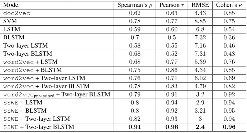
Table 1: Results of the different models on the Kaggle dataset. All resulting vectors were trained using linear regression. We optimized the parameters using a separate validation set (see text) and report the results on the test set.

Since the search space would be massive for grid search, the best hyperparameters were determined using Bayesian Optimization (Snoek et al., 2012). In this context, the performance of our models in the validation set is modeled as a sample from a Gaussian process (GP) by constructing a proba-bilistic model for the error function and then ex-ploiting this model to make decisions about where to next evaluate the function. The hyperparame-ters for our baselines were also determined using the same methodology.

All models are trained on our training set (see Section 4), except the one prefixed ‘word2vecpre-trained’ which uses pre-trained em-beddings on the Google News Corpus. We re-port the Spearman’s rank correlation coefficientρ, Pearson’s product-moment correlation coefficient

r, and the root mean square error (RMSE) be-tween the predicted scores and the gold standard on our test set, which are considered more appro-priate metrics for evaluating essay scoring systems (Yannakoudakis and Cummins, 2015). However, we also report Cohen’sκwith quadratic weights, which was the evaluation metric used in the Kag-gle competition. Performance of the models is shown in Table 1.

In terms of correlation, SVMs produce com-petitive results (ρ = 0.78 and r = 0.77), out-performing doc2vec, LSTM and BLSTM, as well as their deep counterparts. As described

above, the SVM model has rich linguistic knowl-edge and consists of hand-picked features which have achieved excellent performance in similar tasks (Yannakoudakis et al., 2011). However, in terms of RMSE, it is among the lowest performing models (8.85), together with ‘BLSTM’ and ‘Two-layer BLSTM’. Deep models in combination with word2vec(i.e., ‘word2vec+ Two-layer LSTM’ and ‘word2vec+ Two-layer BLSTM’) and SVMs are comparable in terms of r and ρ, though not in terms of RMSE, where the former produce better results, with RMSE improving by half (4.79). doc2vecalso produces competitive RMSE results (4.43), though correlation is much lower (ρ= 0.62andr = 0.63).

The two BLSTMs trained withword2vec em-beddings are among the most competitive models in terms of correlation and outperform all the mod-els, except the ones using pre-trained embeddings andSSWEs. Increasing the number of hidden lay-ers and/or adding bi-directionality does not always improve performance, but it clearly helps in this case and performance improves compared to their uni-directional counterparts.

fair comparison as these are trained on a much larger corpus than our training set (which we use to train our models). Nevertheless, when we use our SSWEs models we are able to outper-form ‘word2vecpre-trained + Two-layer BLSTM’, even though our embeddings are trained on fewer data points. More specifically, our best model (‘SSWE+ Two-layer BLSTM’) improves correla-tion toρ = 0.91andr = 0.96, as well as RMSE to2.4, giving a maximum increase of around10% in correlation. Given the results of the pre-trained model, we believe that the performance of our best

SSWE model will further improve should more training data be given to it.7

5.2 Discussion

Our SSWE + LSTM approach having no prior knowledge of the grammar of the language or the domain of the text, is able to score the essays in a very human-like way, outperforming other state-of-the-art systems. Furthermore, while we tuned the models’ hyperparameters on a separate vali-dation set, we did not perform any further pre-processing of the text other than simple tokeniza-tion.

In the essay scoring literature, text length tends to be a strong predictor of the overall score. In order to investigate any possible effects of essay length, we also calculate the correlation between the gold scores and the length of the essays. We find that the correlations on the test set are rela-tively low (r= 0.3, ρ= 0.44), and therefore con-clude that there are no such strong effects.

As described above, we used Bayesian Op-timization to find optimal hyperparameter con-figurations in fewer steps than in regular grid search. Using this approach, the optimization model showed some clear preferences for some parameters which were associated with better scoring models:8 _{the number of ‘noisy’ sequences}

E, the weighting factor α and the size of the LSTM layer DLST M. The optimal α value was

consistently set to0.1, which shows that ourSSWE

approach was necessary to capture the usage of the words. Performance dropped considerably as

α increased (less weight onSSWEs and more on the contextual aspect). When usingα = 1, which 7_{Our approach outperforms all the other models in terms}

of Cohen’sκtoo.

8_{For the best scoring model the hyperparameters were as}

follows: D = 200, H = 100, η = 1e−7, n = 9, E = 200, α= 0.1, DLST M = 10, r= 0.5.

is equivalent to using the basic C&W model, we found that performance was considerably lower (e.g., correlation dropped toρ= 0.15).

The number of ‘noisy’ sequences was set to 200, which was the highest possible setting we considered, although this might be related more to the size of the corpus (see Mikolov et al. (2013) for a similar discussion) rather than to our approach. Finally, the optimal value forDLST M was10(the

lowest value investigated), which again may be corpus-dependent.

6 Visualizing the black box

In this section, inspired by recent advances in (de-) convolutional neural networks in computer vision (Simonyan et al., 2013) and text summa-rization (Denil et al., 2014), we introduce a novel method of generating interpretable visualizations of the network’s performance. In the present con-text, this is particularly important as one advantage of the manual methods discussed in § 2 is that we are able to know on what grounds the model made its decisions and which features are most discrim-inative.

At the outset, our goal is to assess the ‘qual-ity’ of our word vectors. By ‘qual‘qual-ity’ we mean the level to which a word appearing in a particu-lar context would prove to be problematic for the network’s prediction. In order to identify ‘high’ and ‘low’ quality vectors, we perform a single pass of an essay from left to right and let the LSTM make its score prediction. Normally, we would provide the gold scores and adjust the network weights based on the error gradients. Instead, we provide the network with apseudo-scoreby taking the maximum score this specific essay can take9 and provide this as the ‘gold’ score. If the word vector is of ‘high’ quality (i.e., associated with higher scoring texts), then there is going to be lit-tle adjustment to the weights in order to predict the highest score possible. Conversely, providing the minimum possible score (here 0), we can assess how ‘bad’ our word vectors are. Vectors which re-quire minimal adjustment to reach the lowest score are considered of ‘lower’ quality. Note that since we do a complete pass over the network (without doing any weight updates), the vector quality is going to beessay dependent.

9_{Note the in the Kaggle dataset essays from different}

es-say sets have different maximum scores. Here we take as

˜

. . . way to show that Saeng is a determined . . . . . . . sometimes I do . Being patience is being . . .

. . . which leaves the reader satisfied . . .

. . . is in this picture the cyclist is riding a dry and area which could mean that it is very and the looks to be going down hill there looks to be a lot of turns . . . .

. . . The only reason im putting this in my own way is because know one is patient in my family . . . .

. . . Whether they are building hand-eye coordination , researching a country , or family and friends through @CAPS3 , @CAPS2 , @CAPS6 the internet is highly and

I hope you feel the same way .

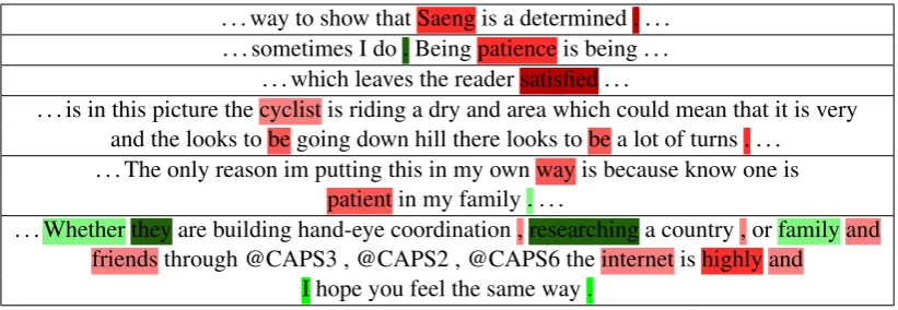
Table 2: Several example visualizations created by our LSTM. The full text of the essay is shown in black and the ‘quality’ of the word vectors appears in color on a range from dark red (low quality) to dark green (high quality).

Concretely, using the network functionf(x)as computed by Eq. (12) – (17), we can approximate the loss induced by feeding thepseudo-scoresby taking themagnitude of each error vector (18) – (19). Since limkwk2→0yˆ = y, this magnitude

should tell us how much an embedding needs to change in order to achieve the gold score (here pseudo-score). In the case where we provide the minimum as apseudo-score, akwk2 value closer

to zero would indicate an incorrectly used word. For the results reported here, we combine the mag-nitudes produced from giving the maximum and minimumpseudo-scoresinto a single score, com-puted asL(˜ymax, f(x))−L(˜ymin, f(x)), where:

L(˜y, f(x))≈ kwk2 (18)

w=∇L(x), ∂L_∂x

(˜y,f(x)) (19)

where kwk2 is the vector Euclidean norm w =

qP_N

i=1wi2;L(·)is themean squared erroras in

Eq. (8); andy˜is the essaypseudo-score.

We show some examples of this visualization procedure in Table 2. The model is capable of providing positive feedback. Correctly placed punctuation or long-distance dependencies (as in Sentence 6 are . . . researching) are particularly favoured by the model. Conversely, the model does not deal well with proper names, but is able to cope with POS mistakes (e.g.,Being patienceor

the internet is highly and . . .). However, as seen

in Sentence 3 the model is not perfect and returns a false negative in the case ofsatisfied.

One potential drawback of this approach is that the gradients are calculated only after the end of the essay. This means that if a word appears

mul-tiple times within an essay, sometimes correctly and sometimes incorrectly, the model would not be able to distinguish between them. Two possi-ble solutions to this propossi-blem are to either provide the gold score at each timestep which results into a very computationally expensive endeavour, or to feed sentences or phrases of smaller size for which the scoring would be more consistent.10

7 Conclusion

In this paper, we introduced a deep neural network model capable of representing both local contex-tual and usage information as encapsulated by es-say scoring. This model yieldsscore-specific word

embeddings used later by a recurrent neural

net-work in order to form essay representations. We have shown that this kind of architecture is able to surpass similar state-of-the-art systems, as well as systems based on manual feature engineer-ing which have achieved results close to the upper bound in past work. We also introduced a novel way of exploring the basis of the network’s inter-nal scoring criteria, and showed that such models are interpretable and can be further exploited to provide useful feedback to the author.

Acknowledgments

The first author is supported by the Onassis Foun-dation. We would like to thank the three anony-mous reviewers for their valuable feedback.

10_{We note that the same visualization technique can be}

References

Yigal Attali and Jill Burstein. 2006. Automated essay scoring with e-Rater v.2.0. Journal of Technology, Learning, and Assessment, 4(3):1–30.

Ted Briscoe, John Carroll, and Rebecca Watson. 2006. The second release of the RASP system. In Pro-ceedings of the COLING/ACL, volume 6.

Ted Briscoe, Ben Medlock, and Øistein E. Andersen. 2010. Automated assessment of ESOL free text examinations. Technical Report UCAM-CL-TR-790, University of Cambridge, Computer Labora-tory, nov.

Ciprian Chelba, Tom´aˇs Mikolov, Mike Schuster, Qi Ge, Thorsten Brants, Phillipp Koehn, and Tony Robin-son. 2013. One Billion Word Benchmark for Mea-suring Progress in Statistical Language Modeling. InarXiv preprint.

YY Chen, CL Liu, TH Chang, and CH Lee. 2010. An Unsupervised Automated Essay Scoring System.

IEEE Intelligent Systems, pages 61–67.

Ronan Collobert and Jason Weston. 2008. A unified architecture for natural language processing: deep neural networks with multitask learning. Proceed-ings of the Twenty-Fifth international conference on Machine Learning, pages 160–167, July.

Ronan Collobert, Jason Weston, Leon Bottou, Michael Karlen, Koray Kavukcuoglu, and Pavel Kuksa. 2011. Natural language processing (almost) from scratch. Mar.

Scott Crossley, Laura K Allen, Erica L Snow, and Danielle S McNamara. 2015. Pssst... textual fea-tures... there is more to automatic essay scoring than just you! InProceedings of the Fifth International Conference on Learning Analytics And Knowledge, pages 203–207. ACM.

Yann N. Dauphin, Harm de Vries, and Yoshua Bengio. 2015. Equilibrated adaptive learning rates for non-convex optimization. Feb.

Misha Denil, Alban Demiraj, Nal Kalchbrenner, Phil Blunsom, and Nando de Freitas. 2014. Modelling, visualising and summarising documents with a sin-gle convolutional neural network. Jun.

Semire Dikli. 2006. An overview of automated scor-ing of essays. Journal of Technology, Learning, and Assessment, 5(1).

S. Elliot. 2003. IntellimetricTM_{: From here to} valid-ity. In M. D. Shermis and J. Burnstein, editors, Au-tomated Essay Scoring: A Cross-Disciplinary Per-spective, pages 71–86. Lawrence Erlbaum Asso-ciates.

Noura Farra, Swapna Somasundaran, and Jill Burstein. 2015. Scoring persuasive essays using opinions and their targets. InProceedings of the Tenth Workshop on Innovative Use of NLP for Building Educational Applications, pages 64–74.

Alex Graves. 2012. Supervised Sequence Labelling with Recurrent Neural Networks. Springer Berlin Heidelberg.

Michael U. Gutmann and Aapo Hyv¨arinen. 2012. Noise-contrastive estimation of unnormalized sta-tistical models, with applications to natural image statistics. J. Mach. Learn. Res., 13:307–361, Febru-ary.

Karl Moritz Hermann, Tom Koisk, Edward Grefen-stette, Lasse Espeholt, Will Kay, Mustafa Suleyman, and Phil Blunsom. 2015. Teaching machines to read and comprehend. Jun.

S Hochreiter and J Schmidhuber. 1997. Long short-term memory. Neural computation, 9(8):1735– 1780.

Beata Beigman Klebanov and Michael Flor. 2013. Word association profiles and their use for auto-mated scoring of essays. InProceedings of the 51st Annual Meeting of the Association for Computa-tional Linguistics, pages 1148–1158.

Thomas K. Landauer, Darrell Laham, and Peter W. Foltz. 2003. Automated scoring and annotation of essays with the Intelligent Essay Assessor. In M.D. Shermis and J.C. Burstein, editors,Automated essay scoring: A cross-disciplinary perspective, pages 87– 112.

Quoc V. Le and Tomas Mikolov. 2014. Distributed representations of sentences and documents. May. Honglak Lee, Roger Grosse, Rajesh Ranganath, and

Andrew Y. Ng. 2009. Convolutional deep be-lief networks for scalable unsupervised learning of hierarchical representations. Proceedings of the 26th Annual International Conference on Machine Learning ICML 09.

Deryle Lonsdale and D. Strong-Krause. 2003. Auto-mated rating of ESL essays. InProceedings of the HLT-NAACL 2003 Workshop: Building Educational Applications Using Natural Language Processing. Danielle S McNamara, Scott A Crossley, Rod D

Roscoe, Laura K Allen, and Jianmin Dai. 2015. A hierarchical classification approach to automated es-say scoring. Assessing Writing, 23:35–59.

Tom´aˇs Mikolov, Stefan Kombrink, Anoop Deo-ras, Luk´aˇs Burget, and Jan ˇCernock´y. 2011. RNNLM-Recurrent neural network language mod-eling toolkit. InASRU 2011 Demo Session.

Tomas Mikolov, I Sutskever, K Chen, G S Corrado, and Jeffrey Dean. 2013. Distributed representa-tions of words and phrases and their composition-ality. InAdvances in Neural Information Processing Systems, pages 3111–3119.

Ellis B. Page. 1968. The use of the computer in ana-lyzing student essays. International Review of Edu-cation, 14(2):210–225, June.

E.B. Page. 2003. Project essay grade: PEG. In M.D. Shermis and J.C. Burstein, editors,Automated essay scoring: A cross-disciplinary perspective, pages 43– 54.

L.M. Rudner and Tahung Liang. 2002. Automated essay scoring using Bayes’ theorem. The Journal of Technology, Learning and Assessment, 1(2):3–21.

Keisuke Sakaguchi, Michael Heilman, and Nitin Mad-nani. 2015. Effective feature integration for auto-mated short answer scoring. InProceedings of the Tenth Workshop on Innovative Use of NLP for Build-ing Educational Applications.

M Shermis and B Hammer. 2012. Contrasting state-of-the-art automated scoring of essays: analysis. Technical report, The University of Akron and Kag-gle.

Mark D Shermis. 2015. Contrasting state-of-the-art in the machine scoring of short-form constructed re-sponses. Educational Assessment, 20(1):46–65. Karen Simonyan, Andrea Vedaldi, and Andrew

Zisser-man. 2013. Deep inside convolutional networks: Visualising image classification models and saliency maps. 12.

D.D.K. Sleator and D. Templerley. 1995. Parsing English with a link grammar. Proceedings of the 3rd International Workshop on Parsing Technolo-gies, ACL.

Jasper Snoek, Hugo Larochelle, and Ryan P. Adams. 2012. Practical bayesian optimization of machine learning algorithms. Jun.

Swapna Somasundaran, Jill Burstein, and Martin Chodorow. 2014. Lexical chaining for measuring discourse coherence quality in test-taker essays. In

COLING, pages 950–961.

Ilya Sutskever, Oriol Vinyals, and Quoc V. Le. 2014. Sequence to sequence learning with neural net-works. Sep.

Kai Sheng Tai, Richard Socher, and Christopher D. Manning. 2015. Improved semantic representa-tions from tree-structured long short-term memory networks. Feb.

Duyu Tang. 2015. Sentiment-specific representation learning for document-level sentiment analysis. In

Proceedings of the Eighth ACM International Con-ference on Web Search and Data Mining - WSDM '15. Association for Computing Machinery (ACM). D. M. Williamson. 2009. A framework for imple-menting automated scoring. Technical report, Ed-ucational Testing Service.

Helen Yannakoudakis and Ronan Cummins. 2015. Evaluating the performance of automated text scor-ing systems. In Proceedings of the Tenth Work-shop on Innovative Use of NLP for Building Educa-tional Applications. Association for Computational Linguistics (ACL).