Parametric Linear Stochastic Modelling of Benue River flow Process

Parametric Linear Stochastic Modelling of Benue River

Flow Process

Otache Y. Martins, Isiguzo E. Ahaneku, Sadeeq A. Mohanned

Department of Agricultural & Bioresources Engineering, Federal University of Technology, Minna, Nigeria E-mail: [email protected]

Received May 11, 2011; revised May 30, 2011; accepted July 2, 2011

Abstract

The dynamics and accurate forecasting of streamflow processes of a river are important in the management of extreme events such as floods and droughts, optimal design of water storage structures and drainage net-works. In this study, attempt was made at investigating the appropriateness of stochastic modelling of the streamflow process of the Benue River using data-driven models based on univariate streamflow series. To this end, multiplicative seasonal Autoregressive Integrated Moving Average (ARIMA) model was developed for the logarithmic transformed monthly flows. The seasonal ARIMA model’s performance was compared with the traditional Thomas-Fiering model forecasts, and results obtained show that the multiplicative sea-sonal ARIMA model was able to forecast flow logarithms. However, it could not adequately account for the seasonal variability in the monthly standard deviations. The forecast flow logarithms therefore cannot read-ily be transformed into natural flows; hence, the need for cautious optimism in its adoption, though it could be used as a basis for the development of an Integrated Riverflow Forecasting System (IRFS). Since fore-casting could be a highly “noisy” application because of the complex river flow system, a distributed hydro-logical model is recommended for real-time forecasting of the river flow regime especially for purposes of sustainable water resources management.

Keywords:Stochastic Process, Water Resources, Dynamics, River Flow, Modeling

1. Introduction

Inherent in the principles of water resources management is the judicious utilization and conservation of the avail-able water resources. One of the ways to enhance this is the proper estimation of water demand both quantita-tively and qualitaquantita-tively. Within this overall management system, the hydrologist is often required to estimate the magnitude of extreme events, whereas operation of some of the design works is often dependent on reliable esti-mates of flow for an ensuing period of time. Since river is an essential component of the hydrologic cycle, its flow forecasting provides a veritable, and basic informa-tion on a wide range of problems related to the design and operation of the entire river system. A very common constraint encountered in the context of water resources planning is inadequacy of streamflow records. The available streamflows, known as historical records, are often quite short, generally sometimes less than a quarter of a century in length. Thus, a system designed on the basis of the historical record only faces a chance of being

inadequate for the unknown flow sequence that the sys-tem might experience. The historical record comprising a single short series does not cover a sequence of low flows as well as high flows. Hence, the reliability of a system has to be evaluated under these conditions which are not possible with historical records alone.

them together are available when developing a stream-flow forecasting model. Determining an appropriate model structure by trial-and-error process is therefore not always practical [8].

The non-practical determinate nature of model struc-ture for streamflow/river flow forecasting can really be appreciated in a wider context considering the fact that river flow is usually treated as a random process, purely stochastic. The justification is that river flow is a func-tion of precipitafunc-tion and other processes which, at pre-sent level of knowledge, seem to evolve randomly in time and space. Even if the underlying phenomena and their interactions were thoroughly understood, it would not be possible to describe mathematically the rate of discharge in a natural water course without involving unsystematic or unknown effects [9]. Considering the issues involved in river flow studies within the premise of a wider hydrological horizon, it is pertinent to appre-ciate the following seemingly, contemporaneous para-doxes:

1) In the face of the stifling dearth of long and con-tinuous data availability, can realistic generalizations be made from forecasting the dynamics of the Benue River?

2) Considering the complex nature of river flow and the significant variability it exhibits in both time and space, what is the appropriateness of using stochastic method for modelling the Benue River flow process?

To this end, the objective of this study is to model the streamflow process of the Benue River with Autoregres-sive Integrated Moving Average (ARIMA) models, fo-cusing on short term forecasting for the purposes of evaluating suitability of particular model type as a pre-liminary step towards developing an enhanced “River Flow Forecasting System” for the river.

2. Materials and Methods

1) Hydrology of the Benue River

The Benue River is the major tributary of the Niger River. It is approximately 1 400 km long and almost navigable during the rainy season (between July and Oc-tober). Hence, it is an important transportation route in the regions it flows through. Its headwaters rises in the Adamawa Plateau of the Northern Cameroon, flows into Nigeria south of the Mandara Mountains through the east-central part of Nigeria before entering the Niger River at Lokoja (Figure 1a). The wide flood plain is

general climatic pattern. There are definite wet and dry seasons which give rise to changes in river flow and sa-linity regimes. The flood of the Benue River (upper, middle, and downstream) lasts from July to October, and sometimes up to early November.

2)Data Base Management

In this study, historical time series for gauging stations at the base of the Benue River (i.e., Lower Benue River Basin) at Makurdi (7°44′ N, 8°32′ E) was used. A total of 26 years (1974–2000) water stage and discharge data were collected and used. The daily flow data were ag-gregated to monthly and annual data series by taking the average of each month’s flow and calendar year. Simi-larly, the annual maximum and minimum daily average discharges were obtained according to the water year, i.e., months of April to March for the streamflow process.

3) Model Formulation and Forecast Strategy The possibility of fitting a multiplicative seasonal ARIMA model to the logarithms of the monthly flows was examined. The forecasts from this model were compared to forecasting using a conventional Thomas-Fiering model. Comparison of forecast errors was also performed to bring to the fore the suitability of either of the models for forecasting the streamflow process of the river. Model formulation and development was patterned after Box and Jenkins [1], Carlson et al. [11] and McKerchar and Delleur [12].

a) Thomas-Fiering Model

Thomas and Fiering [13] described a linear stochastic model for simulating synthetic flow data. On a monthly basis, this represents the means, standard deviations, serial correlations between successive flows, and the skewness. This model uses a linear regression relation-ship to relate the flow Qt1 in the (t+1)th month, (t be-ing from the start of the generated sequence) to the flow

t in the t(th) month. If

Q Q_j and Q_j1 be the mean

monthly discharges during months j and j+1, respectively, within a repetitive annual cycle of 12 months, bj be the

regression coefficient for estimating the flow in the (j+1)th month from the jth month, and tt be a normal de-viate with zero mean and unit variance, the Thomas- Fiering equation will be







₂



1 2

1 1 1 1

t j j t j t j j

(a)

(b)

[image:3.595.103.493.76.689.2]

1

j

where yt,yt-j, σj and фj represents the transformed (i.e., standardized) series; transformed series at the previous time step, standard deviation of each month, and autore-gressive parameter value of order one for each month, respectively. In the application of the Thomas-Fiering model, negative values are sometimes generated. It is recommended that these values be retained and used to derive the subsequent values in the sequence, and when once the generated sequence is completed, all the nega-tive values in the generated sequence be replaced by zero. Similarly, if there is no occurrence of flow for a particu-lar month, then generation of flow for such a month may not be carried out. Since there is flow all year round in the Benue River, this procedure was ignored.

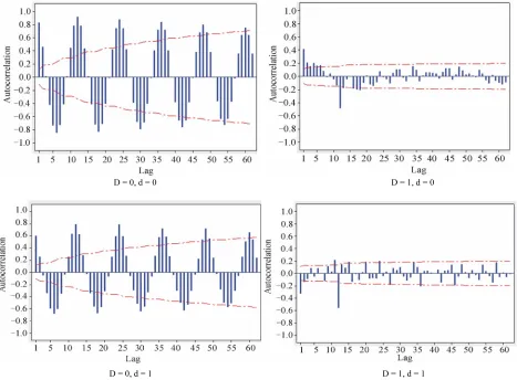
tion function plots for these differencing schemes. To account for runoff phenomenon in the streamflow data, the prospect of seasonal differencing seem more promising since seasonality cannot really be accounted for by non-seasonal differencing, nor is an integrated moving average scheme expected to account for the non-seasonal autoregressive behaviour. Thus considering this factor, a multiplicative ARIMA model



1, 0, 2

 

 1,1,1,



₁₂ was examined. This model has the form







12

 

12



2



1 1,12 1,12 1 2

1B 1 B z_t  1 B 1B B a_t (4) where,

i

, i, and i stand for non-seasonal autoregressive,

D = 0, d = 0 D = 1, d = 0

[image:4.595.66.533.356.700.2]

seasonal autoregressive, and seasonal moving average parameters, respectively; while zt and at are logarithmic transformed series and model random shocks, respec-tively.

c) Flow Forecasting

The ARIMA model was used to forecast flows for one to 24-month ahead. With reference to an origin at time t (here, t = 288), the model was used to make minimum mean square error forecasts of zt+L for , where L is the lead time. The values forecasted for zt+L for an origin at t with lead time L will be written as

1

L



ˆ

t



Z L .

Diagnos-tic verification of the adequacy of the model was done by evaluating the autocorrelation function for the residuals by modifying the model to take into account any non-random features. Figure 3 shows the residual auto-correlation function for model





₁₂ in re-spect of parameter estimation (Table 1) and the final parameter values (Table 2) as well as the corresponding diagnostic check for model adequacy (Table 3). At 5% level of significance, the autocorrelation plot of the model residual reflects that the residual series may be considered random (Figure 3).





[image:5.595.115.486.235.434.2]

1, 0, 2  1,1,1,

[image:5.595.77.518.476.707.2]

Figure 3. Residual autocorrelation function for ARIMA



1,0,2

 

 1,1,1,



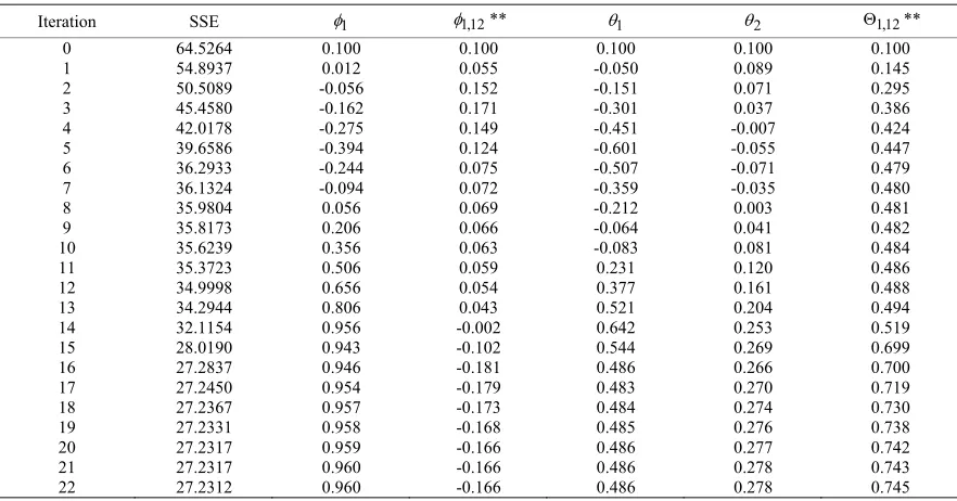
₁₂ model.

Table 1. Estimation of ARIMA model parameters.

Iteration SSE ₁ 1,12** 1 2 1,12**

0 64.5264 0.100 0.100 0.100 0.100 0.100

1 54.8937 0.012 0.055 -0.050 0.089 0.145

2 50.5089 -0.056 0.152 -0.151 0.071 0.295 3 45.4580 -0.162 0.171 -0.301 0.037 0.386 4 42.0178 -0.275 0.149 -0.451 -0.007 0.424 5 39.6586 -0.394 0.124 -0.601 -0.055 0.447 6 36.2933 -0.244 0.075 -0.507 -0.071 0.479 7 36.1324 -0.094 0.072 -0.359 -0.035 0.480

8 35.9804 0.056 0.069 -0.212 0.003 0.481

9 35.8173 0.206 0.066 -0.064 0.041 0.482

10 35.6239 0.356 0.063 -0.083 0.081 0.484

11 35.3723 0.506 0.059 0.231 0.120 0.486 12 34.9998 0.656 0.054 0.377 0.161 0.488 13 34.2944 0.806 0.043 0.521 0.204 0.494

14 32.1154 0.956 -0.002 0.642 0.253 0.519

15 28.0190 0.943 -0.102 0.544 0.269 0.699

16 27.2837 0.946 -0.181 0.486 0.266 0.700

17 27.2450 0.954 -0.179 0.483 0.270 0.719

18 27.2367 0.957 -0.173 0.484 0.274 0.730

19 27.2331 0.958 -0.168 0.485 0.276 0.738

20 27.2317 0.959 -0.166 0.486 0.277 0.742

21 27.2317 0.960 -0.166 0.486 0.278 0.743

22 27.2312 0.960 -0.166 0.486 0.278 0.745

MA 2 0.2782 0.0646 4.31 0.000

SMA 12* 0.7447 0.0544 13.69 0.000

Constant 0.000318 0.001155 0.28 0.783

[image:6.595.74.521.102.187.2]

** Seasonal autoregressive parameter, * seasonal moving average parameter

Table 3. Modified Box-Pierce (Ljung-Box) Chi-Square statistic.

Lag 12 24 36 48

Chi-Square 10.2 29.0 46.3 60.4

Critical value 12.6 28.9 43.8 58.1

DF 6 18 30 42

In terms of the forecasting function, the general ARIMA model can be written in three alternative forms: as a difference equation, an infinite sum of the current and weighted previous values of shocks at, and an infi-nite sum of weighted previous observations plus the cur-rent value of at. Conditional expectation of any of these forms supplies a forecasting function. In this regard, the difference equation was used. By recalling that Z Lt

 





Zt L



, using square brackets to signify conditional

ex-pectation, noting that

 

 

1

1 1

0,1, 2,

ˆ 1, 2,

ˆ 1 0,1, 2,

0

t j t j

t t

t j t t j t j

t j

z z j

z z j j

a a z z j

a                                     1, 2, j   



at

(5)

and taking expectation of the model, which has the general form







12

 

12



2

1 1,12 1,12 1 2

1B 1 B zt  1 B 1B B ,

the forecasting function can be obtained according as:

1 1 1,12 12 1 1,12 13 1 1 2 2 1,12 12 1 1,12 13 2 1,12 14

t L t L t L t L

t L t L t L t L

t L t L

z z z z

a a a a

a a                                      

1 L 24

(6)

Equation (6) can be expanded for the respective lead time (L) to make the forecasts with zt+L, the dependent forecast variable as a function of L. Both the Thomas Fiering and ARIMA models were used to make forecasts of the monthly flow series. Subsequently, the forecasts from the models were compared with the actual flows. Because the last 2 years flow data was used for the com-parison, the parameters were re-estimated for both mod-els for the entire flow series shortened by 2 years (i.e., the model fit was done with 26 years of flow data). The

flow forecasts were considered from the aspect of choosing a particular time origin and taking cognizance of the behaviour of the forecast function as the lead time L increases; that is, the long-term behaviour of the fore-cast function should be a useful theoretical check on the fit of a model. Taking the origin t = 288, forecasts for the logarithms of the flow were made using both models.

3. Results and Discussion

[image:6.595.77.516.228.268.2]

[image:7.595.123.476.88.259.2]

Figure 4. Forecasting for flow logarithms of ARIMA



1,0,2

 

 1,1,1,



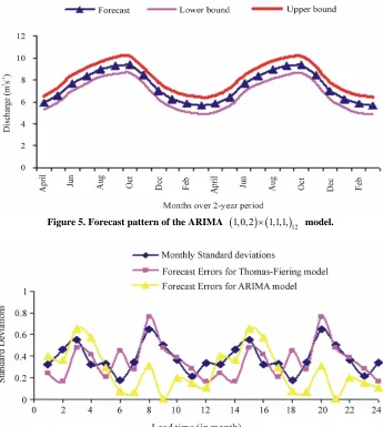
₁₂ model.

Figure 5. Forecast pattern of the ARIMA



1,0,2

 

 1,1,1,



₁₂ model.

[image:7.595.126.471.296.681.2]

[image:8.595.133.466.87.255.2]

Probability of Exceedance or Equalled (%)

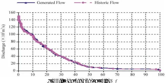
Figure 7. Long-term flow-duration curve of Thomas-Fiering model (Synthetic flow simulation).

particular, it leads to problems in transforming forecasted flow logarithms into natural flows.

4. Conclusions

Based on the results of analysis done, it is evident that autoregressive and ARIMA models have an important place in stochastic hydrology. Specifically, logarithms of monthly flows may be represented either with a low-order autoregressive model (if the series are first standardized) or with a multiplicative seasonal ARIMA model of the order



1, 0, 2

 

 1,1,1,



₁₂ . The stochastic models (Thomas-Fiering and ARIMA



, 2

 

 1,1,1,



₁₂) may be used for forecasting of the Benue River monthly flow, though the former performed relatively better than the later. The ARIMA model was able to forecast flow logarithms, but because it did not adequately account for the seasonal variability in the monthly standard devia-tions, the standard errors associated with the forecasts may not be physically correct. Also, the logarithms can-not be correctly transformed into natural flows; thus giv-ing concern for cautious optimism. However, the sto-chastic modelling does show that the ARMA type mod-els could be used as preliminary modmod-els which may form the basis for understanding the dynamics of the stream-flow process. For the purposes of developing real-time Integrated River flow Forecasting System for the Benue River within the overall context of water resources man-agement strategy, consideration should be given to dis-tributed river flow hydrological models that incorporate hydroclimatic forcing. It suffices to note also that the appropriateness of the stochastic process for every flow series may be debated in the context of nonlinear deter-minism and chaos, according to which seemingly com-plex and irregular behaviours could be the outcome of simple deterministic systems with only a few nonlinear

interdependent variables with sensitive dependence on initial conditions. On this basis, nonlinear deterministic methods could be viable complement to linear stochastic ones for studying river flow dynamics if sufficient cau-tion is exercised in their implementacau-tion and interpreta-tion of results.

1, 0

5. References

[1] L. Garrote and R. L Bras, “A Distributed Model for Real-Time Flood Forecasting Using Digital Elevation Models,” Journal of Hydrology, Vol. 167, No. 1, 1995, pp. 279-306.doi:10.1016/0022-1694(94)02592-Y

[2] J. C. Refsgaard and J. Knudsen, “Operational Validation and Intercomparison of Different Types of Hydrological Models,” Water Resources Research, Vol. 32, No. 7, 1996, pp. 2189-2202.doi:10.1029/96WR00896

[3] E Todini, “The ARNO Rainfall-Runoff Model,” Journal of Hydrology, Vol. 175, No. 2, 1996, pp. 339-382.

doi:10.1016/S0022-1694(96)80016-3

[4] J. Buchtele, V. Elias, M. Tesar and A. Herman, “Runoff Components Simulated by Rainfall-Runoff Models,” Journal of Hydrological Sciences, Vol. 41, No. 1, 1996, pp. 49-60.doi:10.1080/02626669609491478

[5] K. L. Hsu, H. V. Gupta and S. Sorooshian, “Artificial Neural Network Modelling of Therainfall-Runoff Proc-ess," Water Resources Research, Vol. 31, No. 10, 1995, pp. 2517-2530.doi:10.1029/95WR01955

[6] D. Mukherjee and N. Mansour, “Estimation of Flood Forecasting Errors and Flow-Duration Joint Probabilities of Exceedance,” Journal of Hydrologic Engineering, Vol. 122, No. 3, 1996, pp. 130-140.

doi:10.1061/(ASCE)0733-9429(1996)122:3(130)

[7] H. Raman and Sunikumar, “Multivariate Modelling of Water Resources Time Series Using Artificial Neural Networks,” Journal of Hydrological Sciences, Vol. 40, No. 4, 1995, pp. 145-163.

[8] C. M. Zealand, D. H. Burn and S. P. Simonovic, “Short Term Forecasting Using Artificial Neural Networks. Journal of Hydrology, Vol. 214, No. 1-4, 1999, pp. 32-48.

doi:10.1016/S0022-1694(98)00242-X

[9] N. T. Kottegoda, “Stochastic Water Resources Technol-ogy,” The Macmillan Press Ltd, London, 1980, pp. 2-3, 21, 112-113.

[10] G. E. P. Box and G. M Jenkins, “Time Series Analysis Forecasting and Control,” Holden-Day Press, San Fran-cisco, 1976, pp. 32-100.

[11] R. F. Carlson, A. J. A. McCormick and D. G. Watts, “Ap-plication of Linear Random Models to Four Annual Flow

Series,” Water Resources Research, Vol. 6, No. 4, 1970, pp. 1070-1078.doi:10.1029/WR006i004p01070

[12] A. I. McKerchar and J. W. Delleur, “Application of Sea-sonal Parametric Linear Stochastic Models to Monthly Flow Data,” Water Resources Research, Vol. 10, No. 2, 1974, pp. 246-254.doi:10.1029/WR010i002p00246