Optimal Trajectory of Underwater Manipulator Using
Adjoint Variable Method for Reducing Drag
Kazunori Shinohara
JAXA’S Engineering Digital Innovation Center, Japan Aerospace Exploration Agency, Sagamihara City, Japan E-mail: shinohara@06.alumni.u-tokyo.ac.jp
Received June 28,2011; revised July 30, 2011; accepted August 16, 2011
Abstract
In order to decrease the fluid drag on an underwater robot manipulator, an optimal trajectory method based on the variational method is presented. By introducing the adjoint variables, which are Lagrange multipliers, we formulate a Lagrange function under certain constraints related to the target angle, target angular velocity, and dynamic equation of the robot manipulator. The state equation (the partial differentiation of the grange function with respect to the state variables), adjoint equation (the partial differentiation of the La-grange function with respect to the adjoint variables), and sensitivity equation (the partial differentiation of the Lagrange function with respect to torques) can be derived from the stationary conditions of the Lagrange function. Using the state equation, we can calculate the state variables (angles, angular velocities, and angu-lar acceleration) at every time step in the forward time direction. These state variables are stored as data at every time step. Next, by using the adjoint equation, we can calculate the adjoint variables by using these state variables at every time step in the backward time direction. These adjoint variables are stored as data at every time step. Third, the sensitivity equation is calculated by using both the state variables and the adjoint variables. Finally, the optimal trajectory of the manipulator is obtained using the sensitivities. The proposed method is applied to the problem of two-link manipulators. It can obtain the optimal drag reduction trajectory of the manipulator under the constraints mentioned above.
Keywords:Robot Manipulator Dynamics, Optimal Trajectory, Adjoint Variable Method, Euler-Lagrange Equation, Fluid Drag Force, Calculus of Variations
1. Introduction
Presently, we are facing serious environmental problems such as global warming and abnormal climatic condi-tions, which are closely related to the ocean. Therefore, the establishment of ocean study technology is extremely important. Since the 1990s, researchers have investigated the development of underwater robot manipulators for oceanic studies [1-6].
In an extreme environment such as the abyssal ocean, it is difficult to supply energy to manipulators. However, because of fluid tractions, the energy consumption of an underwater manipulator is greater than that of a manipu-lator in air. In order to reduce the energy consumption, it is important to determine the optimal trajectory to reduce the drag on the manipulator.
Optimal time control for a manipulator trajectory was studied in the 1970s [7,8]. Kahn and Roth first presented
an optimal time control method based on kinematic dy-namics [9]. Vukobratovic and Kiranski presented an op-timal time control method based on dynamic program-ming [10]. Townsend et al. presented optimal control by approximating a function [11]. Lee et al. presented the formulation of a genetic algorithm based on trajectory planning [12]. Constantinescu et al. presented a method for determining smooth and time-constrained optimal path trajectories for a robot manipulator [13]. These studies were carried out with the objective of constructing an optimal time trajectory for a manipulator, from its initial position to the target position. On the other hand, Eiji
presented a method for determining the minimum energy trajectory of an underwater manipulator [14]. Uno et al.
presented a minimum torque change model [15]
under an extreme environment is crucial for low energy consumption.
In this study, we propose an optimal trajectory method for reducing the drag on the manipulator. As the ma-nipulator moves from its initial position to the target po-sition, the fluid generates an external force on the ma-nipulator. A method based on the variational principle is developed to determine the optimal trajectory to reduce the drag. This method is called the adjoint variable me- thod. The adjoint variable method is based on a varia-tional method. By introducing Lagrange multipliers called adjoint variables, we transform the constrained optimization of the cost function into the unconstrained optimization of the Lagrange function. The cost function is defined as the fluid drag on the manipulator. The La-grange function is formulated under the constraints of the robot manipulator dynamics. The stationary conditions (the state equation, adjoint equation, and sensitivity equation) are derived from the Lagrange function. An algorithm is developed on the basis of the stationary conditions. First, the state variables (the angle, angular velocity, and angular accelerations) are calculated by using the state equation in the forward time direction and stored as data at every time step. Next, by using the state variables at every time step, we calculate the adjoint variables by using the adjoint equation in the backward time direction. Finally, the sensitivity (gradient) is cal-culated at every time step, and the time history of the joint torques is determined.
Using this optimal trajectory algorithm developed in three phases (state analysis, adjoint analysis, and sensi-tivity analysis), we resolve the problem of the two-link manipulator. The effectiveness of the algorithm is then verified by comparing it with the optimal time control methods described in the literature.
2. Theory
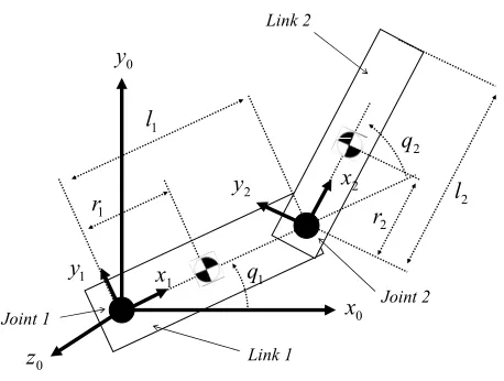
2.1. VariableIn this paper, the two-dimensional motion of a manipu-lator with respect to the x-y plane is considered, as shown in the Figure 1. The links are arranged in the shape of a circular cylinder. The manipulator consists of two links that are connected by joints. The coordinates at each joint are defined. The joints and links are numbered from the base to the tip.
The angles with respect to joint i are defined as
1, 2
q ii (1) The angular velocities with respect to joint i are de-fined as:
1, 2
q ii (2)
1 q
2 q
0 x 0
y
0 z
1 y
1 x
2
y x2
1 r
1 l
2
r 2
l
Joint 2 Joint 1
Link 2
[image:2.595.310.539.81.254.2]Link 1
Figure 1.Two-link manipulator.
The angular accelerations with respect to joint i are defined as
1, 2 q ii
(3)
In this study, the variables obtained from Eq.(1) to Equation (3) are called state variables (q = ( 1 2 1 2
1 2)). The penalty parameters with respect to the angle
and angular velocity are defined as
, , , , q q q q ,
q q
1, 2,3, 4 i
i (4) Variables with respect to the angular accelerations (q q 1, 2) are defined as
1, 2 i
i (5) The variables obtained from Equation (5) are called adjoint variables (λ=(λ1, λ2)). The torques with respect to
joint i are defined as
1, 2 i
i (6) The masses with respect to link i are defined as
1, 2
m ii (7) The diameters with respect to link i are defined as
1, 2
d ii (8) The lengths with respect to link i are defined as
1, 2
l ii (9) The lengths from the centroid of a link to joint i are defined as
1, 2
r ii (10) The drag coefficients with respect to link i are defined as
1, 2
C ii (11) The density of the water is defined as
The translational veloci de
(13) The sign function sgn(x) is def
ties with respect to link i are fined as
1, 2 v ii
ined as
0sgn 0 if 0
1 if 0
x x
x 1 if x
(14)
In order to derive the dynamics of an underwater robot m
em
order to minimize the cost function under certain con-anipulator, the external force exerted by the fluid drag needs to be added to the robot manipulator dynamics. The fluid drag on an object is proportional to the square of the object’s speed [16]. The fluid drag always has a positive value in the calculation of the robot manipulator dynamics. With respect to the motion direction of the manipulator, the fluid drag acts in the opposite direction in a real environment. Therefore, the sign of the fluid drag direction has to be determined according to the mo-tion of the manipulator. The momo-tion direcmo-tion of the ma-nipulator can be identified by the sign of the translational velocities.
.2. Probl 2
In
straints, a Lagrange function is formulated by introduc-ing the adjoint variables. The input data are the time his-tories of the torques (τ1, τ2) from the start time 0to the
end time t. The optimal trajectory is searched for in the set of inputs. After determining the values of τ1 and τ2,
the angle, angular velocities, and angular accelerations are determined using the state equation from start time 0 to the end time t. The tip of the underwater manipulator moves from the initial position to the target position. The objective of this study is to reduce the fluid drag by the 2D trajectory of the manipulator. The cost function is defined as
1 2
J D D N (15)
(16)
2
1 1 2 2 3 1 4 2
1 0 1 1 1
2 0 2 2 2
2 2
3 1 4 2
d 0
d 0
t
t
N q a q b q c q d
q t q a q a
q t q b q b
q c q d
2
2
2
3 2
1 6 1 1 1 1 sgn
D C d l q q1
(17)
2 2
2
2 22
l l
q l l q q
2
2 2 2 2 1 1 2 1 1 2 1 2
2 2 2
2
2 3 3
3
D C d l l l l
l q
(18)
where the parameters a, b, c, and d in Equation (16) are constants. The first and second terms in Equation (16) are the constraints with respect to the target angle a of joint 1 and target angle b of joint 2, respectively. The third and fourth terms in Equation (16) are the con-straints with respect to the target angular velocity c of joint 1 and target angular velocity d of joint 2, respec-tively. Equations (17) and (18) represent the fluid drag on link 1 and link 2, respectively (see Appendix A). In order to simplify the formulation of the adjoint variable method in this study, it is assumed that the inequality
1 1
l q l q2
1q2
0 is satisfied at all times. The La-grange function is defined as1 2 1 1 2 2
D D N F F
L J F (19) where equations F1 and F2 constitute the state equation. This state equation represents the robot manip
quation of the Lagrange function int variable λ is called the state ulator dy-namics. In this study, a weak formulation is applied to the Lagrange function by the time integration of the state equation. The Lagrange function can also be formulated by a strong formulation that satisfies the equation at every time step.
2.3. State Equation
The partial differential e ith respect to the adjo w
equation:
1
1 1 1
d 0 0
L L F L
dt
(20)
2
2 2 2
d 0 0
d
L L F L
t
Equations (20)-(21) represent the robot d nipulator as
(21)
ynamic
ma-
,
M q q C q q f q (22) The parameters M, C, f, and τ represent the i
trix, vector of the coriolis and centrifugal fo
nertia forces, drag rce, and joint torque, respectively. By using the pa-rameters in Appendix B, Eqaution (22) is written as
5
6 2 1 13 1
3
2 2 2 14 2
A
A A q A
A
A B q A
(23)
2 3 2 5 2 14 2 13
1 1
1 1
3 6 2 13 6 14
1 1
2 2
1 1 1
2 6 2 1 1 0 0
2 2 2 5
A A B A A A B
A A
F q
A
F q A A
A A A A A A
A A B A A A A A A A (24)
where parameters A1– A14, B1, and B2 are discussed in Appendix B and Appendix C.
2.4. Adjoint Equations
uler-Lagrange equations erived from the stationary condition of the Lagrange
ons are derived as
The adjoint equations are the E d
function. The adjoint equati
1 1
d 0
d
L L
q t q
(25)
2 2
d
0 d
L L
q t q
(26)
The time derivation of the adjoint variable λ1 is
de-rived from Equation (25) (see Appendix D).
1 1 1 3 1 4 1 5 16
2 10 2 7 2 5 2 16 2 17 1
1 1
2
2 7 10 6 2 17 6 5 2 16 2
1 1
2 2
2
t q a q c B q B A
A A B A A B r A B A
A A
(27)
A A A A A A A B r A
A A
The time derivation of the adjoint variable λ2 is
de-rived from Equaiton (26).
2 2 2 4 2 5 18
2 12 2 5 2 18 2 18 19
1
B A A B r A B A A
1
2 12 2 18 19 6 5 2 18
2
1
2
t q b q d B A
A
A A A A A A B r A
A
The condition of the end time tf is derived from the partial differential equation of the Lagrange function with respect to the state variables as
(28)
1 2
0, 0
f f
L t L t
q q
(29)
0 1,i tf i
2 (30)
2.5. Sensitivity Equations
rtial differential equation of the Lagrange function with respect to the torque τis calle
on: The pa
d the sensitivity equa-ti
1 2 2 2
d B A
L L
1,( )k 0 0
L G t
1 dt 1 A1 1
(31)
1 2 2 6
2,( )
2 2 1 2
d
0 0
d k
A A
L
L L
G t t A (32) where the subscript (k) represents an iteration, as sh in the Figure 2. The time histories of the torques are iteratively modified from the time histories of the initial torques. The algorithm determines the optimal trajectory by minimizing the Lagrange function. Finally, Gi,(k)
own
(t)(I
= 1, 2) reaches zero if the subscript (k) represents a suffi-cient number of iterations.
2.6. Steepest Descent Method
The time histories of the torques are modified by the gradient as
Using Equation (29), we obtain the following equa-tions:
1,k1 t 1, k
t G1, k
t (33)
t
t2,k1 2, k G2, k
t (34)er to robustly converge to the optimal trajec-tory and to avoid numerical vibration and di
this study, the parameter α is set to 0.1.
3.
The data of the every time step are stored in the PC
econd phase, using the state variable at The value of the coefficient α should be sufficiently small in ord
vergence. In
Algorithm
The algorithm is shown in the Figure 2. In the first phase, the state variable (q) is calculated from the start time to
he end time in the forward direction. t
state variable at emory. In the s m
0 (
0 (
q ):Initialcondtions
)
Convergence? condtions Initial
:
) 0 (
) 0 (
λ
:
) (
) ( 1
n k
:
) (
) ( , 2
n k
variables Adjoint
n k n
k, :
) (
) ( , 2 ) (
) ( , 1
Start time
Visualization by Gnuplot YES
NO
YES NO
n=n+1
n=n-1
Torques
n k
i :
) (
) ( ,
Time derivation of adjoint variables Time derivation of adjoint variables
Angles q
q n
k n
k, :
) (
) ( , 2 ) (
) ( , 1
Velocities q
q n
k n
k, :
) (
) ( , 2 ) (
) ( ,
1
ons Accelerati q
q n
k n
k, :
) (
) ( , 2 ) (
) ( , 1
Start time
End time
y Sensitivit G n
k
i :
) (
) ( ,
Sensitivity equations
Eqs.(31)-(32)
Steepest decent method
Eqs.(33)-(34) State equations
Adjoint equations
Table 1
Eq. (24) Obtained by Runge
-Kutta method
Eq.(30)
End time
Eq.(27)
Eq.(28)
Obtained by Runge
-Kutta method
k=k+1
Figure 2. Algorithm.
almost agrees with the target position. In the case where the position of the manipulator does not reach the target position, this algorithm returns to the first phase.
method r reducing the drag on a manipulator. Using this
rag reduction trajectory can be obtained. he optimal trajectory obtained by the drag reduction
optimal trajectory obtained by the time optimal control method described in the literature [17] (see Appendix E).
e time optimal control method, the manipulator requires a minimum amount of time to move from the Using th
4. Results
In Section 2, we formulated the adjoint variable fo
method, the d T
control method can be verified by comparing it with the
initial position to the target position.
4.1. Calculation Conditions
are summarized in
able 1.
origin (0, 0). The aximum and minimum values for both torque 1 and
37, B2 = 0.3033, and B3 = 0.1482 in the
litera-tu
gures show angle 1 and angle 2, respec-vely. Angle 1 (q) constantly converges to the target
s away from e target angle. After that, by rapidly closing to the
tar-itial a
calculation conditions are defined as case 1 and case 2. The initial and objective positions
T
The edge of link 1 is fixed at the m
torque 2 are set to ±30(N) and ±10(N), respectively. The initial parameters are summarized in Table 1. The solver is applied to the Runge-Kutta method. The time span is set to 0.001. The time histories of the initial torques, τi,(k)
(I = 1,2), are constantly defined as zero. The parameters
B1 = 4.53
re [17] are used in the manipulator computing model (see Appendix B). The density ρ is set to 1.0. The drag coefficients, C1 in link 1 and C2 in link 2, with respect to
the circular cylinder are each set to 0.1. The lengths, L1
of link 1 and L2 of link 2, are each set to 1.0. The
diame-ters of the cylinder, d1 and d2, with respect to link 1 and link 2 are each set to0.01. The penalty parameters, ε1 ~ ε4,
are set to 5.
4.2. Computational Results in Case 1
The trajectories for case 1 are shown in the Figure 3
(time optimal control) and the Figure 4 (drag reduction control). The end time is 0.81. The time histories of the angles are shown in the Figure 5. The black and red lines in the fi
ti 1
angle. During the first 0.4 s, angle 2 (q2) i
th
get angle, the time optimal trajectory using the inertia force is created. As shown in the Figure 7, the angular velocities (q q 1, 2) almost become zero at end time tf and
satisfy the constraint condition. In link 1 of the manipu-lator, the angular velocity q1 increases monotonically
during approximately the first 0.4 s. After that, the angu-lar velocity q1 decreases monotonically in order to
sat-isfy q10. In link 2 of the manipulator, the angular
[image:6.595.312.539.87.211.2]velocity q20 from 0 s to 0.4 s. After that, the angular Table 1. In nd target conditions in case 1 and case 2.
Parameter Initial condition Target condition
1
q –π/3 0.0
2
q 0.0 0.0
1
q 0.0 0.0
Case 1
0.0 0.0
Case 2
0.0 0.0 2
q
1
q π/3 0.0
2
q –π/6 × 5 0.0
1
q 0.0 0.0
2
q
–2 –1.8 –1.6 –1.4 –1.2 –1 –0.8 –0.6 –0.4 –0.2 0
0 0.5 1 1.5 2 2.5
Meter (m)
Me
te
r
(m
)
Figure 3. Trajectory of two-link manipulator for time op-timal control in case 1.
–2 –1.8 –1.6 –1.4 –1.2
Me
te
r
( –1
–0.8 –0.6 –0.4 –0.2 0
0 0.5 1 1.5 2 2.5
Meter (m)
m
[image:6.595.311.537.258.400.2])
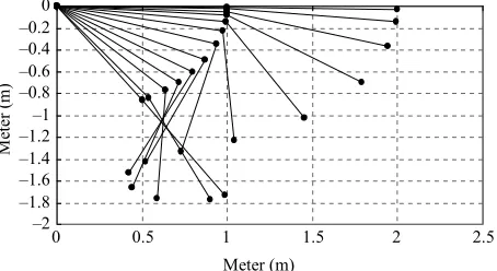
[image:6.595.309.540.444.621.2]Figure 4. Trajectory of two-link manipulator for drag re-duction control in case 1.
Figure 5.Time history of angles for time optimal control in case 1.
velocity , and it decreases in order to satisfy the constraint, 2
0 q
2 q 0
me
[image:6.595.57.286.580.724.2]to meet the end constraint condition, the inverse
maximum torque of –30(Nm) The
maxi-mum torque of –10 (Nm) acts 0.0 s to
0.15 s. After that, the inverse maxim ue of +10 (Nm) acts on joint 2 during 0.19 s - . Again, the maximum torque of –10(Nm) acts on
The drag reduction trajectory and t e history of angles are shown in Figure 4 and Fi pectively. The end time tf is 1.08 s. The angle s a constant value of zero. By avoiding any extr ment of the manipulator, a trajectory from sition to the end position is created for minimum
The time history of the angular vel shown in the Figure 8. Equaiton (40) is angular
ve-locity increases monotonically proximately
The angular velocity to zero
1 0 q , acts on joint 1.
on joint 2 from um torq 0.50 s
joint 2. he tim
gure 6, res
q2 ha
a move the initial po
drag reduction. ocity is satisfied. The
during ap
1
remains close
1 q
y.
the first 0.4 s. After that, in order to satisfy the constraint condition, q 0, angular velocity q decreases
mono-nicall 1
to q2
by adjusting torque 2 at joint 2.
Figure 6.Time history of angles for drag reduction control in case 1.
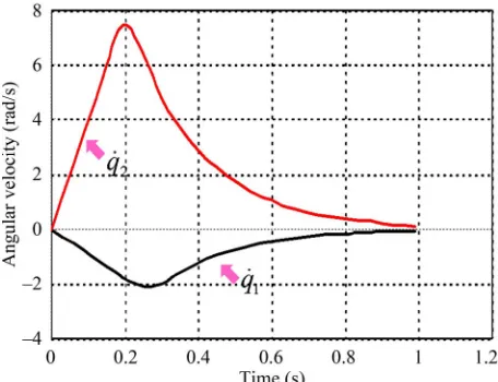
Figure 8.Time history of angular velocities for drag reduc-ion contro
t l in case 1.
Figure 9. Time history of torques for time optimal control in case 1.
The time history of the torques for the drag reduction control is shown in Figure 10. The maximum torque of
+30 (Nm) acts on joint 1 from 0.0 s to0.4 s. After that, by loading the inverse torque, torque 1 is adjusted such that q10
0
. In the case of torque2, in order to satisfy
2
q and q20
positive torque and the negati
, alternative torques using both the ve torque act on joint 2.
4.3. Computational Results in Case 2
For case 2, as shown in Table 1, the trajectory of the manipulator obtained by the time optimal control is shown in the Figure 11. The end time is 0.71 s. The tim
nverges to the target angle. During e first 0.2 s, angle 2 (q2) is away from the target angle.
After that, by rapidly closing to the target angle, a time optimal trajectory is created using the pullback force
e histories of the angles are shown in the Figure 13. The angle q1 constantly co
th
obtained by the inertia force.
The time histories of the angular velocities are shown in the Figure 15. In link 1, the absolute value of the an-gular velocity increases monotonically during ap-proximately th 0.35 s.
After that, the absolute value of angular velocity decreases monotonically in order to satisfy
1 q
e first
1 q 1 0 q
the first .
. A
gular velocity becomes during
s. After that, eter
The tim e t
trajectory are shown in the Figure 17. The maximum torques of +30(Nm) act on joint 1 during approximately the first 0.35 s. After that, the inverse torques act on joint 1 so that
The cl torque 2 acts on joint 2 during the firs
. Again, the clockwise torque takes effect after .45
el
the co ion, a
tra otion of the manipulator, the manipulator is prevented target angle. ink 2 of the manipulator moves in a straight path with
n-0.18
al
2 q
param e histories of t
2 0 q
turns to o
2 q
h 2
0 q
rques for the time-optim
1 0 q .
ockwise t
0.1 s. The counterclockwise torque takes effect from 0.1
s to 0.45 s
0 s.
For case 2, as shown in Table 1, the trajectory of the manipulator obtained by the drag reduction control and the time history of angles for drag reduction control in case 2 are shown in the Figure 12 and the Figure 14, respectiv y. The end time is 1.08 s. In order to reduce
st funct small angle for q2 is selected at every
time step. To prevent the generation of drag by any ex m
from swinging link 2 with respect to the L
respect to the target position.
The time histories of the angular velocities are shown in the Figure 16. Equation (40) is satisfied. The absolute value of the velocities, q1, increases monotonically.
After that, the absolute value of the velocities, q1,
de-creases monotonically in order to satisfy q10.
Angu-lar velocity q2 increases monotonically. After that, q2
[image:8.595.310.539.86.258.2]decreases monotonically in order to satisfy q20.
Figure 10. Time history of torques for drag reduction con-trol in case 1.
M er
M
et
er (m)
et (m)
0 0.5 1 1.5 2 2.5 1
[image:8.595.310.538.305.474.2]0.8 0.6 0.4 0.2 0 –0.2 –0.4 –0.6 –0.8
Figure 11. Trajectory of two-link manipulator for t e op-timal control in case 2.
im
Meter (m)
M
et
er (m)
0 0.5 1 1.5 2 2.5 0.8
[image:8.595.309.539.520.693.2]0.6 0.4 0.2 0 –0.2 –0.4
Figure 12. Trajectory of two-link manipulator for drag- reduction control in case 2.
[image:8.595.59.281.526.693.2]Figure 14. Time history of angles for drag reduction control in case 2.
[image:9.595.57.285.84.256.2]Figure 15.Time history of angular velocities for time opti-mal control in case 2.
[image:9.595.310.536.295.465.2]Figure 16.Time history of angular velocities for drag re-duction con
Figure 17.Time history of torques for time optimal control in case 2.
Figure 18.Time history of torques for drag reduction con-trol in case 2.
ure 18. The clockwise torque 1 takes effect during ap-proximately the first 0.25 s. After 0.25 s, the counter-clockwise torque takes effect. The counter-clockwise and coun-terclockwise torques act alternately. The clockwise torque acts on joint 2 during the first 0.2 s. The counterclock-wise torque takes effect from 0.2 s to 0.4 s. After ap-proximately 0.43 s, the alternative torque acts on joint 2.
5. Conclusions
We proposed the adjoint variable method for obtaining an optimal trajectory in order to decrease the fluid drag on a manipulator when the manipulator moves from its initial position to the target position. By considering hy-drodynamic effects, we formulated the dynamics of an
s the fluid drag. By introducing the adjoint The time histories of the torques are shown in the
Fig-underwater robot manipulator. The cost function was defined a
[image:9.595.58.287.300.473.2] [image:9.595.57.285.518.693.2]ariable, we formulated the Lagrange function under certain constraints, which consisted of the target angle, target angular velocities, and robot manipulator dynam-ics equations. The gradient of the Lagrange function with respect to the torque was derived from the stationary condition. The algorithm was developed on the basis of the adjoint variable method. This algorithm can be suffi-ciently converged to the optimum value under the c straints, and it can determine an optimal trajectory to reduce the fluid drag under the constraints.
Simulation results showed that the performance ca enhanced for the control of an underwater manipulato By using this approach, we can use the motion to reduce fluid drag. It may be important to note that significant performance enhancement is achieved by the motion o
es
v
on-n be r.
f the manipulator.
. Referenc
6
[1] T. L. McLain, S. M. Rock, and M. J. Lee, “Experiments in the Coordinated Control of an Underwater Arm/Vehi-cle System,” Autonomous Robots, Vol. 3, No. 2-3, 1996, pp. 213-232. doi:10.1007/BF00141156
[2] K. N. Leabourne and S. M. Rock, “Model Development of an Underwater Manipulator for Coordinated Arm-Ve-hicle Control,” Proceedings of the OCEANS 98 Confer-ence, Nice France, No. 2, 1998, pp. 941-946.
[3] J. Yuh, S. Zhao and P. M. Lee, “Application of Adaptive erver Control to an Underwater
Manipu-onal Conference on Robotics and
Auto-Disturbance Obs lator,” Internati
mation, Vol. 4,2001, pp. 3244-3249.
[4] S. Sagara, T. Tanikawa, M. Tamura and R. Katoh, “Ex-periments on a Floating Underwater Robot with a Two- Link Manipulator,” Artificial Life and Robotics, Vol. 5, No. 4, 2001, pp. 215-219. doi:10.1007/BF02481505
[5] G. R. Vossoughi, A. Meghdari and H. Borhan, “Dynamic Modeling and Robust Control of an Underwater ROV Equipped with a Robotic Manipulator Arm,” 2004Japan USA Symposium on Flexible Automation, Denver USA, 2004.
[6] K. Ioi and K. Itoh, “Modelling and Simulation of an Un-derwater Manipulator,” Advanced Robotics, Vol. 4, No. 4, 1989, pp. 303-317. doi:10.1163/156855390X00152
[7] M. L. Nagurka and V. Yen “Optimal Design of Robotic
Manipulator Trajectories: A Nonlinear Programming
echnical Report CMU-RI-TR-87-12, the te, Carnegie Mellon University, April,
ia, Philadelphia,
nd Control, Approach,” T
Robotics Institu 1987.
[8] M. Žefran, “Review of the Literature on Time-Optimal Control of Robotic Manipulators,” Technical Report MS- CIS-94-30, University of Pennsylvan
1994.
[9] M. E. Kahn and B. Roth, “The Near Minimum-Time Control of Open-Loop Articulated Kinematic Chains,”
Journal of Dynamic Systems, Measurement a
Vol. 93, No. 3, 1971, pp. 164-172.
doi:10.1115/1.3426492
[10] M. Vukobratović and M. Kirćanski, “A Method for Op-timal Synthesis of Manipulation Robot Trajectories,”
Journal of Dynamic Systems, Measurement, and Control, Vol. 104, No. 2, 1982, pp. 188-193.
doi:10.1115/1.3139695
[11] M. A. Townsend, “Optimal Trajectories and Controls for
pulator with Acceleration Parameterization,”
Jour-and Systems of Coupled Rigid Bodies with Application of Biped Locomotion,” Thesis (Ph.D.), University of Wis-consin Madison,Madison, 1971.
[12] Y. D. Lee and B. H. Lee, “Genetic Trajectory Planner for a Mani
nal of Universal Computer Science, Vol. 3, No. 9, 1997, pp. 1056-1073.
[13] D. Constantinescu and E. A. Croft, “Smooth Time-Optimal Trajectory Planning for Industrial Ma-nipulators Along Specified Paths,” Journal of Robotic Systems, Vol. 17, No. 5, 2000, pp. 233-249.
doi:10.1002/(SICI)1097-4563(200005)17:5<233::AID-R OB1>3.0.CO;2-Y
[14] E. Shintaku, “Minimum Energy Trajectory for an Un-derwater Manipulator and Its Simple Planning Method by Using a Genetic Algorithm,” Advanced Robotics, Vol. 13, No. 6-13, 1999, pp. 115-138.
[15] Y. Uno, M. Kawato and R. Suzuki, “Formation and Con-trol of Optimal Trajectory in Human Multijoint Arm Movement,” Biological cybernetics, Vol. 61, No. 2, 1989, pp. 89-101. doi:10.1007/BF00204593
[16] J. Saleh, “Fluid Flow Handbook,” McGraw Hill, New York, 2002.
the coordinates (x0,y0,z0)
0
Appendix A: Fluid Drag
The underwater manipulator receives a reactive force when it moves to the target position. In this section, the fluid force on the manipulator is derived. In this study, the link is defined as a circular cylinder. The transla-tional velocity with respect to
(=(0,0,0)) of link 1 is given by
1
1 0 1 1 1 1
1
0 0 0
0 0 0
0 0 x x q q
v v ω x (35)
here the variable v0 represents the velocity on the
round. In this study, the base is fixed at v0 = 0. The
ariable ω1 is the angular velocity vector in link 1. The
anslational velocity in link 2 is given by w g v tr
1 21 1 2 1 2
0 0 2 0 0 0 0 0 0
2 1 2 2 1 1
x l q
v v ω x
q q
l q x q q
(36)
Using Equation (35), we obtain the fluid drag in link 1 as
1 2
1 1 0 0 1 1 1 1 1
sgn d
2 l
C d x q x
v ω x 1 2 2
1 1 0 1 1 1 1
0
sgn( ) d 2
l
C d x q x q x
1 0
(37)The function sgn
x q1 1
always becomes the function
1sgn q because x1 > 0. Therefore, sgn
x q1 1
1sgn q The integration in Equation (37) is not related to the function sgn
q1 . Thus, Equation (37) becomes
3 2 3 2
1 1 1 1 1 1 1 1 1 1
1 1
0 0
1
sgn sgn
2 3 6
0 0
0
0
C d l q q C d l q q
D D (38)
The fluid drag in link 2 is (see next page)
In this study, in order to simplify the formulation of the adjoint variable method, it is assumed to satisfy the inequality as
1 1 2 1 2 0
l q l q q (40) n (39) bec
Appen
The variables used in this study can be defined as fol-lows:
2
Thus, Equatio omes (see next page)
dix B: Definition of Variables
2 2 2
1 1 2 2 3 cos
A B B B B q (42)
2 2 22 2 0 1 1 2 1 2 1 1 2 1 2 2
2
2 2 2
2 2 0 1 1 1 1 1 2 2 1 2 2
0 sgn d 2 0 0 2 sgn 2 l l
C d l q x q q l q x q q x
C d l q l q q q x q q x
l q1 1 x q2 1 q2
dx22 2
2 2 0 1 2 2 1 1 2 1 2 2
sgn d
2
l
C d l q x q q x
0
v ω x (39)
2 2 2 22 2 2 2
2 2 2 1 1 2 1 2 1 2 1 2
2
3 3
l
C d l l l l q l l l q q 2 2
2
sgn d
3
l l
C d l q x q q x q
2 2 0 1 2 2 1 1 2 1 2 2
2 0 2 0 0
v ω x 2
2 2 3cos
A B B q (43)
2 2
3 3 1sin
A B q q (44)
2 2
4 2 3 1 2cos 2 3 2cos
A B q q q B q q (45)
2 2
5 2 3 1 2sin 2 3 2sin
A B q q q B q q (46)
2 6 1 2 3cos
A B B q (47)
2 7 2 3 2sin
A B q q (48)
2 8 3sin
A B q (49)
2 9 3cos
A B q (50)
10 3 1sin 2
A B q q (51)
2
11 3 1cos 2
A B q q (52)
in
12 2 3 1 2 s 2
A B q q q (53)
2 2
13 4 1 5 2 5 1cos 2 6 1 7 1 2 8 2 2 A B q B r B l q B q B q q B q
(54)
214 5 2 6 1 7 1 2 8 22
A B r B q Bq q B q (55)
15 5sin 2 6 12 7 1 2 8 22
A B q Bq B q q B q (56)
16 2 6 1 7 2
A B q B q (57)
17 2 4 1 5 2 5 1cos 2
2 6 1 7 2
A B q B r B l q B q B q (58)
18 7 1 2 8 2
A B q B q (59)
19 5 2 5 1cos 2
A B r B l q (60) where the variables B1 – B8 are defined as follows:
2 2 1 m l
1 1 2
1 1 1
2 2
1 1
1 1 1 2 2 2 2 1
16 12
zz zz
zzg
B I I
I m r
d l m (61)
2 2 2
2 2 2 2 1
zzg
I m r m l
2 2
2 d2 l2 2 2
m r m m r m l
16 12
2 2
2 2 2 2
2 2 2 2 2 2 2
16 12
zz zzg
d l
B I I m r m m r
2
1
(62)
3 2 2
B m r l (63)
3
4 1 1 1 sgn( )1
6
B C d l q (64)
5 2 2
B C d2 2l (65)
2
2 2
6 1 1 2
3
l B l l l
(66)
2
7 2 1
2 3
B l l l
2 (67)
2 2
8 3
l
B (68)
Appendix C: Robot Manipulator Dynamics
The translational acceleration, a1, of the barycenter in
link 1 is as
1 1 1 1 1 1
2
1 1
1 1
1 1 1
0 0 0
0 0 0 0 0
0 0
r r
r q
q q q
a ω r ω ω r
1 1
0
r q
(69)
The translational acceleration a2 of the barycenter in
link 2 is given by
2
2 1 1 2 2 2 2 2
2
2 2 1 1
1 2
2
1 2 1 2
sin cos 0 0 0
0 0 1 0
0 0
0 0 0
0
q q l q
q q r
q q q q
2 2 1 1 2
cosq sinq 0 l q 0 r
0
a R e ω r ω ω r
2 2
1 1 2 1 2 2 2 1 2
2
1 1 2 1 1 2 2 1 2
cos sin
sin cos
0
l q q l q q r q q
l q q l q q r q q
(70) The vect
with respect to the tip o sents the rotation matri
coordinates (x1,y1,z1). The translational forces f1 and f2
with respect to l
2
or ei represents the angular acceleration vector f link i. The matrix R1
repre-x from coordinates (x2,y2,z2) to
2
ink 1 and link 2 are given by
2m2 2
f a D (71)
1
1 1 2 2 1
m
1 a R f D (72)
f
1
where the matrix represents the rotation matrix from the coord
(x2,y2,z2).
1
2
R
inates (x1,y1,z1) to the coordinates
2 2
1 sinq cosq 0
2 2 2
cos sin 0
0 0
q q
R (73)
2 (74)
where the first and second terms on the right-are
2 2 2 2 I2 2 2
n I a ω ω f r
hand side
2
2 1 2 2 1 2
0 0 0 0
x
z z
I
2 2 0 2 0 0 0
0 0
y I
I q q I q q
I
α (75)
22 2 2 2
1 2 2 1 2
0 0 0 0
0 0 0 0
0 0 0
x y
z
I I
q q I q q
ω Iω
0 0 (76) where the matrix I2 represents the inertia tensor of lin
The vector α2 represents the acceleration of link 2.
equilibrant moment at joint 1 is derived as
(77)
where the matrix I1 represents the inertia tensor of link 1.
Th
The adjoint equations are derived. The v are k 2. The
1 11 2 2 1 1 2 2 1 1
1 1 1 1 1
n R n f r R f r l
Iα ω Iω
e vector α1 represents the acceleration of link 1. With
respect to the z axis, moments n1 of the joint 1 and n2 of
the joint 2 are defined as torques τ1and τ2. Equation (24)
is thus derived.
Appendix D. Derivation of Adjoint Equations
ariables q1, q2, 1
q , q2, q1, and q2 independent of each other. The
partial differential equation of the Lagrange function with respect to q1 is given by
1 0 1 3 1 4 1
1
2 10 2 7 2 5 2 16 2 17
1
5 16
1 1
1d 2 2
2
t
L t q a q c B q B A
q
A A B A A B r A B A
A
(78) 1 12 7 10 6 2 17 6 5 2 16
2
2
A A
A A A A A A A B r A A
The partial differential equation of the Lagrange func-tion with respect to q1 is given by
1 1 L q
(79)
The partial differential equation of the Lagrange func-tion with respect to q2 is given by
2 0 2 4 2
2
1d 2
t
L t q b q d B A
q
2 12 2 5 2 18 2 18 19
1
1
2 12 2 18 19 6 5 2 18
2
1
B A A B r A B A A
A
A A A A A A B r A
A (80)
The partial differential equation of the Lagrange func-tion with respect to q2 is given by
2 2 L 5 18 q
(81)
Appendix E. Derivation of Adjoint Equations
. The parameters are defined as follows: The time optimal control method is described in the lit-erature [17]. The Hamiltonian formulation is applied in time optimal control. Using a Legendre transformation, the Hamiltonian formulation is derived from the
Lagran-ian formulation g
1 1
x q (82)
2 1
x q (83)
3 1
x q (8 )
4 2
4
x q (85) The state equation is defined as
3
1 4 1
2 2 3 2 5 2 2 2
1 2
1 1 1
3 3
4 2 5 3 6 2 6 4
1 2
1 1 1
d d
x
x x S
x A A B A B A S
A A A
x S
t
x A A A A A A S
A A A
(86)
The cost function with respect to the time optimal con- trol is given by
0 d 01d
t t
J
L t N
t N t N (87)where the constraint N represe and Equation (16). Using the a 3, 4), the Hamiltonian is defined as
nts the constraint condition djoint variables pi (i = 1, 2,
T
H p SL (88) where L represents 1 of the integrand in Equation (87). The adjoint equation is given by
T
T Td d H L t p p S
x x (89)
The boundary condition of the adjoint equ given by ation is
T f f f N t p t t xx (90)
The Hamiltonian Equation (89) is
1 3 2 4 3 3 4
1
H p x p x p S pS (91)
1
H 1
d d
0
p (92)
t x
Using Equation (89), the adjoint equation is given by
2 3 2 5
8 9
3 6
8 92 4 3 8 2 11
3
1
2
A A A A A
p p p
A
2 5
2 4 5 8 2 3 8 6 11 2 A
A A A A A A A A
2 2
1 1
2 8 9 8 2 8 9 8
3 1 3 2
2 2
1 1
1 1
d
2 2
t A A
B A A A A A A A
p p
A A
A A
2
d B A A A A A A A B A A A
4 2
1
A
2 8 9 8
4 1 2
1 1
2
A A A A
p
A
A
6 8 9 4 2 2
1
2A A A p H
A
x2
(93)
2 7 2 10 2 7 6 10
4
A A A A
3 1 3
1 1 3
2 2
d d
B A A A H
p p p
t A
p
A x (94)
2 12 2 6
A A B A
2 12 2 2
4
1 4
d d
B A B A H
4 2 3
1
p p p
t A p
A x
(95)
The constraint condition at the end time is given by
1 f 2 1 1 f
p t x t a (96)
2 f 2 2 2 f
p t x t b
(97) 0)
(98)
The gradient is given by
2
B H
p p 2
3 4
1 1
1
3 4
2 1
A
3 f 2 3 3 f (
p t x t c
4 f 2 4 4 f ( 0)
p t x t d (99)
6 2
1
A A
A
H A
p p
A A
(100)