Lateral Shear Layer and Its Velocity Distribution of Flow in Rectangular Open Channels

(1)

DOI: 10.4236/jamp.2019.74056 Apr. 16, 2019 829 Journal of Applied Mathematics and Physics

Lateral Shear Layer and Its Velocity

Distribution of Flow in Rectangular Open

Channels

Xiaonan Tang

Department of Civil Engineering, Xi’an Jiaotong-Liverpool University, Suzhou, China

Abstract

The lateral velocity distribution of flow in the shear layer of open channel is required to many problems in river and eco-environment engineering, e.g. distribution of pollutant dispersion, sediment transport and bank erosion, and aquatic habitat. It is not well understood about how the velocity varies laterally in the wall boundary layer. This paper gives an analytical solution of lateral velocity distribution in a rectangular open channel based on the depth-averaged momentum equation proposed by Shiono & Knight. The ob-tained lateral velocity distributions in the wall shear layer are related to the two hydraulic parameters of lateral eddy viscosity (λ) and depth-averaged secondary flow (Γ) for given roughened channels. Preliminary relationships between the above two parameters and the aspect ratio of channel, B/H, are obtained from two sets of experimental data. The lateral width (δ) of the shear layer was investigated and found to relate to the λ and the bed friction factor (f), as described by Equation (26). This study indicates that the lateral shear layer near the wall can be very wide (δ/H = 14.6) for the extreme case (λ

= 0.6 and f = 0.01).

Keywords

Lateral Shear Layer, Velocity Distribution, Analytical Model, Lateral Width, Open Channel Flow, Secondary Flow

1. Introduction

In open channel flow, like natural rivers and canals, flows are of highly three-dimensional characteristics owing to the influence of boundaries, varying roughness and non-uniform shapes. Even modeling flow in straight prismatic

How to cite this paper: Tang, X. (2019) Lateral Shear Layer and Its Velocity Dis-tribution of Flow in Rectangular Open Channels. Journal of Applied Mathematics and Physics, 7, 829-840.

https://doi.org/10.4236/jamp.2019.74056

Received: March 15, 2019 Accepted: April 13, 2019 Published: April 16, 2019

(2)

DOI: 10.4236/jamp.2019.74056 830 Journal of Applied Mathematics and Physics

channels becomes surprisingly difficult, as shown by Chiu & Chiou [1] and Nezu & Nakagawa [2]. This is partly due to the nature of the anisotropic turbulence, which is generated by various factors, such as variations in channel geometry and roughness, the consequent formation of secondary flow cells, and the level of turbulence closure.

Due to the complexity of three-dimensional flow, under certain assumptions, one- or two-dimensional analyses are often used in engineering practice. Lots of research has been studied on velocity vertical distribution in open channel flows

[2] [3] [4] [5], which could not meet the requirement of lateral velocity distribu-tion in engineering applicadistribu-tion. The lateral velocity distribudistribu-tion is pre-requisite in solving certain problems in open channel flows, such as lateral distribution of pollutant, sediment transport and aquatic habitat [6]. However, there is not an analytical formula for predicating the lateral velocity distribution of flow in a rectangular channel.

This paper provides an analytical solution of lateral velocity distribution in the shear layer of rectangular channels, which have various aspect ratios, based on the depth-averaged flow model proposed by Shiono & Knight [7] [8]. Shiono and Knight’s model has a wide range of application for curved channels [9], compound weirs [10] [11] and compound channels [12] [13]. The obtained ana-lytical solution of lateral velocity distribution is related to three parameters: the eddy viscosity parameter (λ), secondary flow term (Γ) and the bed friction factor (f). Through analysis on the analytical velocity distribution, it was found that the lateral extent of the shear layer is related to the eddy viscosity parameter (λ) and the bed friction factor (f). An empirical relationship was also established by ana-lyzing two sets of experimental data from Knight et al.[14] and Atabay [15], also see www.flowdata.bham.ac.uk. The results of the lateral width of the shear layer indicate that the shear layer near the wall could be very wide for natural rivers when the λ is very large.

In the following sections, Section 2 provides theoretical background with the assumption of model and its analytical solution, followed by experimental data used for model parameter evaluation in Section 3. Section 4 shows the detailed comparison between the analytical model and experiment, along with the discus-sion on the lateral extent of shear layer. Some concludiscus-sions are given in Section 5.

2. Theoretical Consideration

2.1. Introduction

For steady flow in a prismatic open channel, the governing momentum equation in the stream wise direction may be combined with the continuity equation to give [8] [16]:

( )

(

)

τ

ρ

_∂ + ∂ _=

ρ

+∂ +∂

∂ ∂ ∂ ∂

 

yx zx

o

UV UW gS

y z y z (1)

where U, V, W are the time-averaged velocity components in the x (streamwise),

(3)

[image:3.595.298.448.74.234.2]

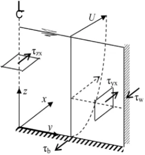
Figure 1. Streamwise Reynolds stress in an open channel.

bed slope, ρ is the density of water, and g is the gravitational acceleration. τyx and τzxdenote the turbulent shear stresses on the planes perpendicular to the y and z

directions, respectively. The left terms of Equation (1) thus signify the secondary flow per unit weight, which is balanced by the weight component and both the lateral and vertical Reynolds stresses in x direction.

For steady flow in a rectangular channel, consider that W z H= =W z=0 =0

and by integrating Equation (1) over the water depth (H), the depth-averaged momentum equation can be obtained as (Shiono & Knight [8]):

(

ρ

)

ρ

∂

(

τ

)

τ

∂ _  =_ + −

∂ ∂

yx

o b

d

H

H UV gHS

y y (2)

where τb is the bed shear stress, the overbar or subscript d denotes the

depth-averaged value, and

(

)

1 ₀

(

)

d

ρ =

_∫

H ρ

d

UV UV z

H (3)

(

)

0 1

d

τ =

_∫

H −ρ

yx uv z

H (4)

in which u and v are the fluctuating velocity component in x and y direction re-spectively. Through an eddy viscosity concept, the Reynolds stress, τyx, can be

described as:

τ =ρε ∂ ∂

d

yx yx

U

y (5)

*

εyx =λU H (6)

where λ is the dimensionless eddy viscosity coefficient and U* (= τ ρb ) is the

local shear velocity. The bed shear stress, τb, may be related to the depth-averaged

velocity, Ud, using the Darcy-Weisbach friction coefficient (f), which is

2 8

τ

_{=  }

ρ

 

 

b d

f

U (7)

(4)

* 8 = f _d

U U (8)

Then, inserting Equations (5) and (7) into (2) gives:

(

)

2 2 2

8 2 8

ρλ

ρ ρ ρ  ∂ 

∂ _ _{ =} ₋   ₊ ∂       ∂   ∂ _ ∂ _ d o d d U

f H f

H UV gHS U

y y y (9)

Experimental results by Shiono & Knight [8] demonstrate that in overbank flow the term of secondary flow, H(ρUV)d, varies almost linearly with y in the

main and floodplain regions of a channel. Therefore, the lateral gradient of the secondary flow force may be approximated as

(

ρ

)

∂ _  = Γ_ ∂ H UV d

y (10)

where Γ is a dimensionless constant of secondary flow, which varies in different flow regions (Knight et al.[17]). Thus Equation (9) can be expressed by:

2 2

2

8 2 8

ρλ

ρ −ρ  _{ } +_∂∂  ∂_∂ = Γ

 

d

o d

U

f H f

gHS U

y y (11)

which is the governing equation of depth-averaged flow in the streamwise direc-tion.

2.2. Analytical Solution for

U

d 2

For given channels, when f, λ and Γ are fixed values, Equation (11) becomes a standard ordinary differential equation in terms of variable 2

d

U . An analytical

solution to Equation (11) can be obtained under appropriate boundary condi-tions. The detailed solution process is given by Knight et al. [17]. The solutions for the channel with linearly varying bed can also refer to Knight & Shiono [18]

and Tang & Knight [13] [19] for further details.

In a rectangular channel, which has the constant depth of flow (i.e.H = con-stant), the analytical solution of Ud to Equation (11) has the following form:

(

)

1 2

1e 2e

γ −γ

= y+ y+

d

U A A k (12)

where

(

)

8

1 β = gHSo −

k

f (13)

1 4 1 2 8

γ

λ

  = _{ }   f

H (14)

β ρ

Γ =

o

gHS (15)

where A1 and A2 are two integral constants, which can be obtained by applying

the boundary conditions of flow continuity and the no-slip condition at the wall, as shown by Knight et al.[20] [21]. For a simple rectangular channel of semi-width,

(5)

[image:5.595.314.433.72.134.2]

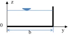
Figure 2. Half rectangular channel cross-section.

( )

1 2

2 cosh

γ

= = − k

A A

b (16)

Thus for a rectangular channel, Equation (12) becomes

( )

cosh

γ

= +

d

U C y k (17)

where

( )

cosh

γ

= −

C k b (18)

3. Experimental Data for Parameter Evaluation

3.1. Calibration of Coefficients and Modelling Philosophy

Strictly speaking, Equation (15) suits for the flow region of constant depth where a constant Γ value exits. If Γ varies laterally, the cross section of a channel can be split into a discrete number of panels if necessary. Generally, panel junctions coincide with the place where the roughness of channel bed or flow depth is discontinuous. Thus, for a symmetric uniform rectangular channel, only half the channel needs to be modeled because of symmetry of the channel. If complex secondary flow cells present, then further division of the channel into more pa-nels may be required [21].

The friction coefficient is generally assumed to be constant in each panel, and it can be back calculated from

=

₈

τ

( )

ρ

2

b d

f

U

_{based on experimental data.}

Note that the variation of λ has great effect for open-channel flows due to lateral shear near wall [22]. Hence, both the secondary flow parameter (Γ) and lateral eddy viscosity coefficient (λ) require calibration in modeling the lateral distribu-tion of depth-averaged streamwise velocity.

3.2. Experimental Data in the Study

The data of lateral flow velocity used herein were obtained from Knight et al. [14] and Atabay [15]. These experiments have covered a wide range of aspect ra-tios (B/H), which vary from 1.0 to 16.0. The earlier experiments by Knight et al. [14] were conducted in a non-tilting 15 m long flume with a rectangular cross-section of width B =152 mm and a bed slope So of 9.66 × 10−4. The more

recent experiments by Atabay [15] were undertaken in a 22 m long flume with a channel width of 50 mm and a bed slope of 2.024 × 10−3_{. These data are also}

ac-cessible from www.flowdata.bham.ac.uk.

(6)

[image:6.595.287.460.76.212.2]

Figure 3. Sketch of half rectangular channel.

Table 1. Parameters adopted in the application of Equation (17).

Experiment B/H f λ Γ MAPE (%)

DWK 0.99 0.0205 0.0003 0.093 1.34

1.38 0.0205 0.0005 0.54 0.98

1.77 0.0205 0.001 0.42 0.73

4.20 0.016 0.015 0.25 5.70

4.79 0.016 0.02 0.15 4.97

AS 6.60 0.019 0.025 0.1 3.72

9.30 0.02 0.038 0.02 2.36

11.86 0.023 0.048 0.008 3.49

15.18 0.026 0.055 0.006 2.93

AS denote the experimental runs by Knight et al. [14] and Atabay [15], respec-tively. In the modelling, ρ = 1000 kg/m3_and_g_{= 9.807 m/s}2_.

4. Results

4.1. Prediction of Lateral Distributions of

Ud

For given parameters of f, λ and Γ, Equation (17) can predict the lateral variation of depth-averaged velocity. Figure 4 and Figure 5 show the lateral distributions of Ud between the prediction and experimental data. The results show that the

prediction by Equation (17) agrees well with the experimental data for flows in rectangular open channels, which have a wide range of aspect ratios (B/H).

To evaluate the robustness of Equation (17) against the experimental data, er-ror analyses were carried out. MAPE (Mean Absolute Percentage Erer-ror) is used as a measure of the error percentage for predicted values of model against the measured values. The individual differences are called as residuals for the data sample that is used for estimation, and the residuals are known as estimation errors for the sample [23] [24] [25].

[image:6.595.210.540.262.432.2]

(7)

[image:7.595.258.491.74.234.2]

Figure 4. Ud distributions for the experiments by Knight et al. [14].

Figure 5. Ud distributions for the experiments by Atabay [15].

, , ,

, − = a i e i u i

e i

u u

E

u (19)

where Eu,i is the error percentage of predicted velocity; ua,i and ue,i are the

pre-dicted and observed velocity at ith measured point (y), respectively. Therefore, the average error percentage of model for an experiment can be computed by

( )

, 1 1

=

∑

N

u i u i

E E

N (20)

where N is the total number of obervation in an experiment.

The values (Eu) of MAPE for all experiments are shown in Table 1, which

shows that the prediction by Equation (17) has the averaged percentage error of 1% to 6%.

[image:7.595.229.518.266.496.2]

(8)

the aspect ratios of channel, as expressed by:

(

)

2

exp

2.36 8.22

,

0.9

93 λ

=



_−

−

B H

_

R

=

(21)

(

)

{

}

(

)

2

0.09 0.174 ln B H 0.924 B H ,R 0.992

Γ = − + + = ₍₂₂₎

where B is the width of channel, H is the flow depth, and R is the correlation coefficient.

4.2. Lateral Extent of Shear Layer

From the analytical solution of Ud, given by Equation (17), it reveals that the

depth-averaged velocity has little change in the major central part of channel, but it decreases rapidly toward zero at the wall, as shown in Figure 4 & Figure 5. With increasing the aspect ratio (B/H) of channel, the extent of almost constant flow velocity is getting wider in the central channel, which can be treated as one-dimensional uniform flow.

When a channel is shallow and very wide, i.e. the ratio of B/H is very large, the value of cosh(γb) in Equation (18) can be very large (∞), so that the C valve in Equation (17) becomes a very small value (close to zero). Note that the second-ary flow is weak in such a shallow channel, thus Γ is negligible (Knight et al. [21]). Therefore Equation (17) becomes:

8 = =

d o

g

U k HS

f (23)

The obtained Equation (23) is the well-known velocity formula for one-dimensional (1-D) uniform flow, i.e. Darcy-Weisbach equation.

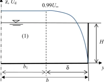
In open channel flow, a lateral shear layer exists near the wall. The extent of lateral shear layer can be defined by a lateral distance, δ, away from the wall, for which

U

_{d y b}_{= −}_δ

=

0.99 U

_∞_.U_∞_{is the velocity of 1-D flow, given by Equation (23),}

as illustrated in Figure 3. The boundary distance δ in the shear layer can be ob-tained as follows:

Applying Equation (17) for Ud

( )

δ =0.99U∞ = k when y = b − δ gives:

(

)

0.99 k = Ccosh_γ b−δ _+k (24a)

or

(

)

0.9801

k

=

C

cosh



_

γ

b

− 

δ



+

k

(24b)

Inserting Equation (18) into (24b) yields

( )

cosh

γδ

−tanh

γ

b ×sinh

γδ

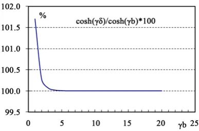
=0.0199 (25)

Since the parameter (γ), given by Equation (14), is a function of depth, Equa-tion (25) is implicit for δ. However, δ can be obtained numerically by solving Equation (25), as graphically shown in Figure 6. This implies that when γb is about 5 the value of Ud at y = b − δ is approximate to 0.99U∞. In other words, in

(9)

[image:9.595.276.470.69.197.2]

Figure 6. The boundary distance (δ) for Ud = 0.99U∞.

Therefore, replacing γ in Equation (14) for γδ = 5 gives:

1 4 1 4

8 8

5 3.54

2

δ λ  _λ 

= _{ } = _{ }

   

H f f (26)

Samuels [26] obtained the similar boundary distance (δ) to Equation (26) with a coefficient 3.4 rather than 3.54 here.

In order to estimate the shear layer width (δ) for a natural river, it needs to es-timate the eddy viscosity coefficient (λ). When bed generated turbulence domi-nates the lateral momentum transfer, Cunge et al.[27] suggested that the typical value of λ is 0.5, which represents the value for the cross-sectional exchange coefficient in the range of 0.23 to 0.6. By taking the extreme case where λ = 0.6 and f = 0.01, Equation (26) gives δ/H ≈ 14.6.

In practical applications for open channel flows, within the boundary width (γδ = 5) Equation (17) can be used to predict the Ud distribution in the lateral

shear layer near the wall, whereas the velocity is calculated by Equation (23) in the central region of channel beyond the shear layer. In fact, the flow in the cen-tral part is uniform flow if the channel is very shallow (i.e. large aspect ratio B/H).

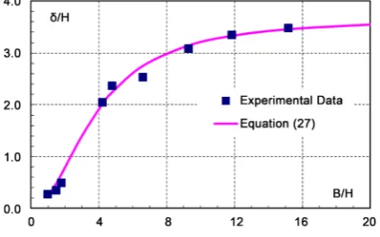
By taking the values of f and λ from Table 1, Equation (26) will establish a re-lationship between δ/H and B/H, as shown in Figure 7. The relationship can be described as:

(

)

2 2

1 0.272 3.982 , 0.994

δ

 



= _ + =

H B H R (27)

5. Conclusions

The depth-averaged velocity distribution in lateral shear layer in a rectangular open channel can be described by Equation (17), which is analytically obtained based on the depth-averaged momentum equation proposed by Shiono & Knight. The analytical solution of Equation (17) agrees well with the experimen-tal data with the aspect ratios ranging from 1 to 16. The percentage error in MAPE is 1% to 6%.

(10)

[image:10.595.267.479.76.208.2]

Figure 7. Plot of δ/H based on Equation (27).

aspect ratios of channel. It reveals that the boundary width can be very large: e.g.

δ/H = 14.6 for the extreme case (λ = 0.6 and f = 0.01) in natural rivers.

The obtained Equation (17) for the lateral velocity distribution was obtained for a rectangular open channel with uniform boundary, but it can be extended to use for velocity analysis in an open channel with non-uniform boundary, where the channel can be split to serial panels of having similar roughness to apply for. Future work may need to establish the relationships (21) & (22) for estima-tions of λ and Γ in channels with heterogeneous roughness, along with the mod-el application on fimod-eld data if available.

Acknowledgements

The author would like to acknowledge the support by the Research Development Funding (RDF-15-01-10), Key Program Special Fund (KSF-E-17) of XJTLU and by the National Natural Science Foundation of China (11772270).

Conflicts of Interest

The author declares no conflicts of interest regarding the publication of this pa-per.

References

[1] Chiu, C.L. and Chiou, J.D. (1986) Structure of 3-D Flow in Rectangular Open Channels. Journal of Hydraulic Engineering, 112, 1050-1068.

https://doi.org/10.1061/(ASCE)0733-9429(1986)112:11(1050)

[2] Nezu, I. and Nakagawa, H. (1993) Turbulence in Open-Channel Flow. IAHR Mo-nograph, Balkema.

[3] Bonakdari, H., Larrarte, F., Lassabatere, L. and Joannis, C. (2008) Turbulent Veloc-ity Profile in Fully-Developed Open Channel Flows. Environmental Fluid Mechan-ics, 8, 1-17. https://doi.org/10.1007/s10652-007-9051-6

[4] Castro-Orgas, O. and Dey, S. (2011) Power-Law Velocity Profile in Turbulent Boundary Layers: An Integral Reynolds-Number Dependent Solution. Acta Geo-physica, 59, 993-1012. https://doi.org/10.2478/s11600-011-0025-1

(11)

Struc-DOI: 10.4236/jamp.2019.74056 839 Journal of Applied Mathematics and Physics

[7] Shiono, K. and Knight, D.W. (1988) Two-Dimensional Analytical Solution for a Compound Channel.Proceedings of 3rd International Symposium on Refined Flow Modelling and Turbulence Measurements,Tokyo, Japan, 26-28 July 1988, 503-510. [8] Shiono, K. and Knight, D.W. (1991) Turbulent Open Channel Flows with Variable

Depth across the Channel. Journal of Fluid Mechanics, 222, 617-646.

https://doi.org/10.1017/S0022112091001246

[9] Tang, X. and Knight, D.W. (2015) The Lateral Distribution of Depth-Averaged Ve-locity in a Channel Flow Bend. Journal of Hydro-Environment Research, 9, 532-541. https://doi.org/10.1016/j.jher.2014.11.004

[10] Zahiri, A., Tang, X. and Azamathulla, H.M. (2014) Mathematical Modelling of Flow Discharge over Compound Sharp-Crested Weirs. Journal of Hydro-Environment Research, 8, 194-199. https://doi.org/10.1016/j.jher.2014.01.001

[11] Zahiri, A., Tang, X. and Sharifi, S. (2017) Optimal Prediction of Lateral Velocity Distribution in Compound Channels. International Journal of River Basin Man-agement, 15, 257-263. https://doi.org/10.1080/15715124.2017.1280813

[12] Tang, X. and Knight, D.W. (2008) Lateral Depth—Averaged Velocity Distribution and Bed Shear in Rectangular Compound Channels. Journal of Hydraulic Engi-neering, 134, 1337-1342.

[13] Tang, X. and Knight, D.W. (2009) Analytical Models for Velocity Distributions in Open Channel Flows. Journal of Hydraulic Research, 47, 418-428.

https://doi.org/10.1080/00221686.2009.9522017

[14] Knight, D.W., Demetriou, J.D. and Hamed, M.E. (1984) Boundary Shear in Smooth Rectangular Channels. Journal of Hydraulic Engineering, 110, 405-422.

[15] Atabay, S. (2001) Sediment Transport in Two Stage Channels. PhD Thesis, Univer-sity of Birmingham, Birmingham, West Midlands, UK.

[16] Knight, D.W. and Tang, X. (2008) Zonal Discharges and Boundary Shear in Pris-matic Channels. Proceedings of the Institution of Civil Engineers: Engineering and Computational Mechanics, 161, 59-68.

https://doi.org/10.1680/eacm.2008.161.2.59

[17] Knight, D.W., Hazlewood, C., Lamb, R., Samuels, P.G. and Shiono, K. (2018) Prac-tical Channel Hydraulics: Roughness, Conveyance and Afflux. 2nd Edition, CRC Press/Balkema, Taylor & Francis Group, London, UK.

[18] Knight, D.W. and Shiono, K. (1996) River Channel and Floodplain Hydraulics. In: Anderson, M.G., Walling, D.E. and Bates, P.D., Eds., Floodplain Processes, Chapter 5, Wiley,Hoboken, NJ, 139-181.

[19] Tang, X. and Knight, D.W. (2008) A General Model of Lateral Depth-Averaged Ve-locity Distributions for Open Channel Flows. Advances in Water Resources, 31, 846-857. https://doi.org/10.1016/j.advwatres.2008.02.002

(12)

DOI: 10.4236/jamp.2019.74056 840 Journal of Applied Mathematics and Physics [21] Knight, D.W., Omran, M. and Tang, X. (2007) Modelling Depth-Averaged Velocity and Boundary Shear in Trapezoidal Channels with Secondary Flows. Journal of Hydraulic Engineering, 133, 39-47.

[22] Chlebek, J. and Knight, D.W. (2006) A New Perspective on Sidewall Correction Procedures, Based on SKM Modelling. Proceedings of the International Conference on Fluvial Hydraulics, Lisbon, Portugal, 6-8 September 2006, 1-10.

[23] Tang, X. (2017) An Improved Method for Predicting Discharge of Homogeneous Compound Channels Based on Energy Concept. Flow Measurement and Instru-mentation, 57, 57-63. https://doi.org/10.1016/j.flowmeasinst.2017.08.005

[24] Tang, X. (2017) Comparison of Different Methods for Predicting Zonal Discharge of Straight Heterogeneously Roughened Compound Channels. Proceedings of the

37th IHAR World Congress, Kuala Lumpur, Malaysia, 13-18 August 2017, 154-163. [25] Tang, X. (2019) A New Apparent Shear Stress-Based Approach for Predicting Dis-charge in Uniformly Roughened Compound Channels. Flow Measurement and In-strumentation, 65, 280-287. https://doi.org/10.1016/j.flowmeasinst.2019.01.012

[26] Samuels, P.G. (1988) Lateral Shear Layers in Compound Channels. International Conference of Fluvial Hydraulics, Budapest, 31 May-3 June 1998, 254-262.