Parameters Influencing the Optimization Process in Airborne Particles PM10 Using a Neuro Fuzzy Algorithm Optimized with Bacteria Foraging (BFOA)

ISSN Online: 2163-0356 ISSN Print: 2163-0283

DOI: 10.4236/ijis.2019.93005 Jul. 31, 2019 67 International Journal of Intelligence Science

Parameters Influencing the Optimization

Process in Airborne Particles PM10 Using a

Neuro-Fuzzy Algorithm Optimized with

Bacteria Foraging (BFOA)

Maria del Carmen Cabrera-Hernandez,

Marco Antonio Aceves-Fernandez

_,

Juan Manuel Ramos-Arreguin, Jose Emilio Vargas-Soto, Efren Gorrostieta-Hurtado

Faculty of Engineering, Universidad Autónoma de Querétaro, Cerro de las Campanas S/N, Querétaro, Mexico

Abstract

The airborne pollutants monitoring is an overriding task for humanity given that poor quality of air is a matter of public health, causing issues mainly in the respiratory and cardiovascular systems, specifically the PM10 particle. In this contribution is generated a base model with an Adaptive Neuro Fuzzy Inference System (ANFIS) which is later optimized, using a swarm intelli-gence technique, named Bacteria Foraging Optimization Algorithm (BFOA). Several experiments were carried with BFOA parameters, tuning them to achieve the best configuration of said parameters that produce an optimized model, demonstrating that way, how the optimization process is influenced by choice of the parameters.

Keywords

Air Pollution, Bacterial Foraging Optimization Algorithm (BFOA), Swarm Intelligence, ANFIS

1. Introduction

The present work proposes a method to model the particulate matter concentra-tions using the BFOA; this method is considered as a novel method since it has not been found in the literature an application of the BFO algorithm in the problem of modeling the concentration of particulate material. Likewise, anoth-er contribution of the present work is to demonstrate how the adjustment of the parameters of the algorithm affects the result and the way in which each of these

How to cite this paper: Cabre-ra-Hernandez, M.C., Aceves-Fernandez, M.A., Ramos-Arreguin, J.M., Vargas-Soto, J.E. and Gorrostieta-Hurtado, E. (2019) Parameters Influencing the Optimization Process in Airborne Particles PM10 Using a Neuro-Fuzzy Algorithm Optimized with Bacteria Foraging (BFOA). International Journal of Intelligence Science, 9, 67-91. https://doi.org/10.4236/ijis.2019.93005

Received: June 25, 2019 Accepted: July 28, 2019 Published: July 31, 2019

Copyright © 2019 by author(s) and Scientific Research Publishing Inc. This work is licensed under the Creative Commons Attribution International License (CC BY 4.0).

http://creativecommons.org/licenses/by/4.0/

DOI: 10.4236/ijis.2019.93005 68 International Journal of Intelligence Science

parameters individually influences said results.

The methodology is basically to use BFOA as optimizer of a base model gen-erated with another technique, ANFIS. The model gengen-erated with ANFIS presents some inaccuracies since it is unstable with highly non-linear problems such as the one that is to be modeled in this work. This is why this method was devised where the accuracy of the base model is improved. Once the model op-timized with BFOA is generated, it will be compared against that generated with ANFIS.

The use of an algorithm that has several agents or swarm intelligence, such as BFOA, gives us the opportunity to find an optimal solution since it involves sev-eral, relatively simple agents exploring the study area, thus having a greater probability of finding the optimal global values avoiding the problem of getting stuck in a local solution as it happens with other methods such as neural net-works, as well as being robust, flexible systems without central control that is-sues orders to system agents [1].

To better understand what the problem is, it is important to define some con-cepts, which are presented below.

1.1. Air Quality

Air quality is an essential issue for humanity since the industrial age, and nowa-days it is more relevant than ever. Although pollutant concentrations are de-creasing worldwide, since countries such as Japan, United States and Brazil, showed a decrease in the concentration of pollutants, there are still less devel-oped countries that have the poorest air quality [2].

The pollutants that are monitored include gases such as ozone (O3), nitrogen

dioxide (NO2), sulfur dioxide (SO2) and particulate matter (PM2.5 and PM10) [3].

The risks of air pollution not only include pulmonary diseases like asthma or even lung cancer, but also the effects of the air pollution, which are related to the appearance of cardiovascular disease, specifically, the pollution of particulate matter, because of its size, which is in the order of the micrometers [4][5].

The particulate matter is classified as PM2.5, which is 2.5 μm (micrometers) of aerodynamic diameter, and PM10, which has 10 μm of diameter; this diameter makes them suitable to be inhaled by humans, causing even deaths on the vul-nerable population [6]. In this contribution, the PM10 concentration in Mexico City is modeled.

1.2. PM10 Modeling

DOI: 10.4236/ijis.2019.93005 69 International Journal of Intelligence Science

ARNN [9]. However, neural networks are not the only technique used for mod-eling PM10. Techniques such as fuzzy logic type 2 [10] and in the field of the swarm intelligence, the ant colony optimization algorithm (ACO) for PM10, Ni-trogen Dioxide and Ozone forecasting [11]. Also ACO in combination with Neuro Fuzzy algorithms applied on CO and O3 forecasting [12]. In addition the

Particle Swarm Optimization, PSO [13] have also been applied to obtain a pre-cise model for the concentration of polluting particles, where the technique showed good performance and is one of the recent works for the particulate matter modeling. PSO belongs to the swarm intelligence algorithms, the same as BFOA, that is why is expected to demonstrate that a swarm intelligence algo-rithm is capable to generate an accurate model for the problem of PM10 beha-vior. In addition, if it turns out to be capable, the goal is to prove which one of the swarm intelligence algorithms that have been implemented can originate the best model for the PM10 pollutant.

1.3. Swarm Intelligence

The social organisms like ants, bees and bacteria colonies perform common tasks as a society like gather food, nest building, among other tasks, for the well-ness of the community, also, have the ability of self-organization forming decen-tralized swarms. The term Swarm Intelligence (SI), first appeared in the late 80’s of the last century [14], the SI algorithms are based on a group of simple agents that interact between them and their environment, this with the objective of achieving a cooperative behavior and more complex than what each agent could individually achieve. These algorithms are mainly inspired by natural pheno-mena such as the colonies of Ants [15], bees [16] or bacteria, water droplets [17], the behavior of bats [18], termites [19], among others.

In this contribution, a Bacterial Foraging Optimization Algorithm (BFOA) is used to model the behavior of PM10 in Mexico City.

Bacterial Foraging Optimization Algorithm

The process of foraging of the Escherichia Coli Bacteria inspires the Bacterial Foraging Optimization Algorithm (BFOA) [20]. The way these bacteria per-forms the process of foraging and reproduction maximizes the energy obtained from the environment.

BFOA have been already accepted as an optimization algorithm and its effi-ciency has been demonstrated in several areas. For instance, its application in the electric engineering a control field [21], pattern recognition [22], PID design

DOI: 10.4236/ijis.2019.93005 70 International Journal of Intelligence Science

The following sections of this paper present the materials and methods for the development of the environmental particle concentration PM10 behavior model, explaining where the data used comes from and how they are used in the gener-ation of the optimized model, as well as a detailed explangener-ation of the methodol-ogy developed for this application. Finally, the results are presented explaining how the adjustment of the parameters of the BFOA algorithm was made, as well as its final configuration to obtain an optimized model.

2. Materials and Methods

2.1. Materials

The data used to build the model were obtained from the Atmospheric Moni-toring System (“Sistema de Monitoreo Atmosférico”, SIMAT) [30], which is re-sponsible for the permanent measuring of the air quality in México City and the metropolitan area. SIMAT has a subsystem; the Automatic Network for Atmos-pheric Monitoring (RAMA), this system uses continuous measuring equipment for air pollutants, such as sulfur dioxide, carbon monoxide, nitrogen dioxide, ozone, PM10 and PM2.5.

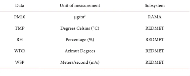
Likewise, atmospheric data were taken from the Meteorology and Solar Radi-ation Network (REDMET), which is a subsystem of SIMAT. From the REDMET, the data of temperature (TMP), relative humidity (RH), wind direc-tion (WDR) and wind speed (WSP) are used. These data are part of the factors for modeling the pollutant concentration [31]. Table 1 contains information about the data used to construct the model and their units of measurement.

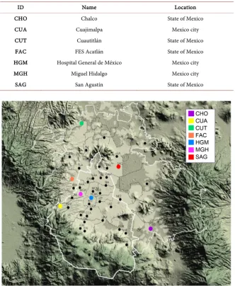
SIMAT has monitoring stations distributed over different areas of the city. These monitoring stations collect information on concentrations of pollutants and atmospheric conditions every hour. Figure 1, shows the monitoring stations available in Mexico City and its surrounding area (called metropolitan area). The criterion for the selection of the stations whose data were used for the con-struction of the model, was taking into account those that had more validated data, since some stations reported invalid data when their measuring instru-ments failed. The stations are listed in Table 2.

The model was validated using data from the same stations of 2015 and data of the year 2017 to evaluate the model performance.

Table 1. Data to build the model.

Data Unit of measurement Subsystem

PM10 µg/m3 _RAMA

TMP Degrees Celsius (˚C) REDMET

RH Percentage (%) REDMET

WDR Azimut Degrees REDMET

DOI: 10.4236/ijis.2019.93005 71 International Journal of Intelligence Science Table 2. ID of the stations.

ID Name Location

CHO Chalco State of Mexico

CUA Cuajimalpa Mexico city

CUT Cuautitlán State of Mexico

FAC FES Acatlán State of Mexico

HGM Hospital General de México Mexico city

MGH Miguel Hidalgo Mexico city

SAG San Agustín State of Mexico

Figure 1. Monitoring stations.

2.2. Building the Model

The approach of this work is the optimization of an existing model (base model), applying the bacterial foraging optimization algorithm as an optimization me-thod.

The main idea about optimizing the model is taking an existing model, which its accuracy can be improved using it as a start, namely, the base model, the proposed technique to generate this base model is an adaptive neuro fuzzy infe-rence system (ANFIS). Fuzzy logic has been used in the past as an optimization method [32].

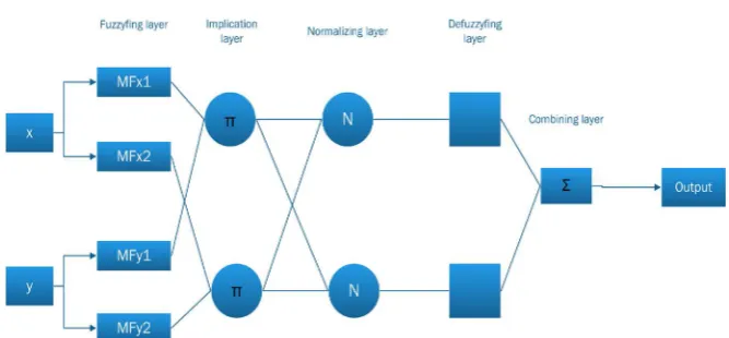
ANFIS is a type of artificial neural network that includes a Takagi-Sugeno fuzzy inference system, that kind of systems have been used in the past for real-time object identification [33], and which is shown in Figure 2.

DOI: 10.4236/ijis.2019.93005 72 International Journal of Intelligence Science Figure 2. ANFIS structure.

input/output, and the membership functions parameters are adjusted using a backpropagation algorithm or in combination with a least squares method.

A FIS can be defined as a set of fuzzy rules of the type IF-THEN, which are expressions with the form IF A THEN B, where A and B are the labels of fuzzy sets [34][35].

As an example, suppose that we have two inputs (x, y) and an output, f, and has five layers to construct the model. Each layer has several nodes that can be adaptive (squared nodes) or fixed (circled nodes) [36].

Layer 1. It is the fuzzy layer and converts the inputs of the model into fuzzy sets by means of membership functions (MF) and the functions of the node are described as:

( )

1,i Ai 1 for 1,2

O =µ X i= ₍₁₎

( )

1 2

1,i B 1 for 3,4

O =µ ₋ Y i= ₍₂₎

where X1 and Y1 are the input nodes, A and B correspond to the linguistic

labels associated with these nodes, µ

( )

( )

functions (MF), the parameters of this layer are called premise parameters. Layer 2. The nodes in this layer are fixed; the function of each node is multip-lied by the input signals, which serves as an output signal and are labeled with Π.

( )

( )

2,i i Ai 1 B 1 for 1,2

O =w =µ X ⋅µ ₋ Y i= ₍₃₎

where O2,i is the output of the layer, and wi represents the firing strength of

the rule.

Layer 3. In the layer the nodes are also fixed, they are labeled with N; its func-tion is to normalize the firing strength, calculating the proporfunc-tion of the ith fir-ing strength to sum the firfir-ing strength of all the rules.

3,

1 2

for 1,2

i

i w

O w i

w w

= = =

+ (4)

where O3,i is the output of the layer 3,

w

strength.

DOI: 10.4236/ijis.2019.93005 73 International Journal of Intelligence Science

4,i i i for 1,2

O =w f⋅ i= ₍₅₎

where f1 y f2 represent the fuzzy rules IF-THEN that are defined like this:

Rule 1. IF X1 is A1 and Y1 is B1, THEN f1= p X1 1+q Y r1 1+ 1

Rule 2. IF X1 is A2 and Y1 is B2, THEN f2= p X2 1+q Y r2 1+ 2

where p qi, i y ri are parameters that are already set and denoted as

conse-quent parameters.

Layer 5. The nodes are fixed and labeled with ∑, their function is to calculate the total output and is defined by:

5,i i i i i i i out total output

i

w f

O w f f

w = =

⋅

=

∑

∑

ANFIS has a very simple learning rule, the backpropagation; this rule calcu-lates recurrently the error signals, starting from the output layer (Layer 5) to the input layers (Layer 1).

2.3. Model Optimization

The BFO algorithm mimics the process of foraging of a real bacterium, whose locomotion is achieved through the movement of its flagella that helps the bac-terium to swim or tumble; these operations are basic in the foraging process. If the flagella rotate in a clockwise direction it generates a tumble movement, in a noxious environment the bacteria will tumble more to find nutrients and when the flagella rotate counterclockwise the bacterium makes a swim, in a suitable environment for the bacterium the swimming movement travels greater dis-tances [37]. The tumble and swim are part of the chemotaxis process, where the bacteria will seek to move in an environment with nutrients while avoiding harmful areas. In Figure 3 the movements of tumble and swimming are shown.

DOI: 10.4236/ijis.2019.93005 74 International Journal of Intelligence Science

When a bacterium finds enough nutrients and the environment has the ade-quate temperature, the bacterium will reproduce dividing in two and creating a replica of itself, forming a colony of bacteria. Likewise, if an attack occurs or the environment suddenly changes, a group of bacteria is dispersed to other areas of the environment or is eliminated; this event is called elimination-dispersion.

Suppose that we want to find the minimum of J(θ) where

θ

p-dimensional vector) and we ignore the nature of the gradient ∇J

( )

we do not know with an analytical description nor measurements of ∇J

( )

BFOA implements an imitation of the main mechanisms present in an actual bacteria E, Coli colony: chemotaxis, formation of the colony or swarming, re-production and elimination-dispersion events, with which the problem of opti-mization without gradient can be solved. The way to explain what a virtual bac-terium represents is that a bacbac-terium is a test solution that moves on the func-tional surface to locate the global optimum [26].

In order to implement the BFO algorithm is essential to define some terms, as an example, a chemotactic step as a tumble followed by a swim, or a tumble fol-lowed by a tumble. Then j is the index of the chemotaxis steps, k is the index of the reproduction steps, and lastly l is the index of the elimination/dispersion events.

The algorithm has certain parameters that must be initialized and on which depends the performance of the algorithm. So let be:

p: Dimension of the search space S: Number of bacteria in the population Nc: Chemotactic steps

Ns: Length of swim Nr: Reproduction steps

Ne: Dispersal-elimination events

Ped: Probability that a bacterium will be eliminated or dispersed C(i): Size of the step taken in a random direction specified by the turn.

Let then _{P j k l}

(

)

(

)

member in the population of S bacteria in the jth step of chemotaxis, the k-th step of reproduction and the l-th elimination-dispersion event, then we can as-sociate a cost J j k l

(

)

(

)

Next, each of the stages of BFOA is described:

Chemotaxis: Suppose that _θi

(

)

each member in the population of S bacteria in the j-th chemotactic step, the k-th step of reproduction and the l-th elimination-dispersion event and C(i) is the step taken in a random direction specified by the tumble, then the movement of artificial chemotaxis is represented by:

(

)

(

)

( )

( )

( ) ( )

T

, , , ,

i _{j k l} i _{j k l C i} i

i i

θ

θ

∆

= ∆

∆

+ ₍₇₎

be-DOI: 10.4236/ijis.2019.93005 75 International Journal of Intelligence Science

tween [−1,1].

Swarm. The real cells respond to chemical stimuli to form groups of cells and thus travel in the environment. Cell-to-cell signals are represented as follows:

(

)

(

)

(

)

(

)

(

)

(

)

attractant attractant 1

2

repellant repellant 1

, , ,

exp

exp

cc

S p i

m m

i l m

S p i

m m

i l m

J P j k l

d w h w θ θ θ θ θ = = = =   = _− − − _     + _− − − _  

∑

∑

∑

∑

where Jcc is the value added to the objective function which is going to be

mi-nimized, wattractant is the quantification of the diffusion rate of the attractant, attractant

d is a quantification of the attraction agent to be released. In the same way, a cell repels any nearby cell in the sense that it is not physically possible to have two cells in the same location. To model this is used the height of the re-pellent hrepellant, which is the magnitude of its effect and whose value is defined

as hrepellant =dattractant and wrepellant is the measure of the diffusion rate of the

re-pellent. These coefficients must be chosen in an appropriate way according to our search space.

The function presented in (8) represents how at the location of each cell as you move radially away from the cell, the function decreases and then increases. This with the purpose of modeling how distant cells will tend not to be attracted, while nearby cells will tend to try to scale the nutrient gradient from cell to cell with each other and, therefore, try to form a swarm. Is important to make clear that as the cell moves, so does its function representing the release of chemicals as it moves. Due to the movements of all the cells, the function varies with time, and if many cells gather, there will be a large amount of attractant, therefore, a greater probability that other cells will move towards the group forming the swarm.

Reproduction. The general criterion for this stage is that the less healthy bac-teria must die while the healthiest bacbac-teria, which are the ones that have a lower value in the objective function, will be reproduced by dividing them in two, keeping the size of the population constant.

Elimination/dispersion. To simulate dispersion and elimination events, a group of bacteria is randomly eliminated with a small probability, and replace-ments are initialized randomly over the search space.

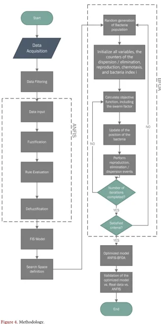
2.4. Methodology

Below are presented the steps of the methodology to obtain the optimized model (Figure 4).

1) Acquisition of data: The raw data to create the model are obtained from a database.

2) Data filtering: The database contains some data that is not valid or that could be partial and must be filtered to avoid having a biased model.

DOI: 10.4236/ijis.2019.93005 77 International Journal of Intelligence Science

into the model.

4) Fuzzification: It is the process of converting the input data into a linguistic value; this depends on the membership functions. In this case, generalized membership functions were used in the form of a bell. The bell function depends on three parameters a, b and c, and is given by.

(

)

1

b

f x a b c

x c a = − + (9)

Evaluation of the rules: the rules of the model are evaluated with respect to the fuzzy rules and the values of the membership functions.

5) Defuzzification: The defuzzification method used was the weighted average of all rule exits.

6) Model Fuzzy inference system: Once the evaluation and defuzzification steps have been completed, the model is constructed with the specific equations of ANFIS expressed in the construction section of the model.

7) Definition of the search space: A search space is defined as all feasible solu-tions within our problem, which is why our search space must first be located between the valid data for environmental factors. Relative humidity, tempera-ture, direction and wind speed as well as within the feasible values of PM10, be-cause given the nature of the problem, another way to define the search space is very difficult since the possibilities are very broad.

8) Generation of the population: the population with S bacteria must be gen-erated, in initial random positions within a range of possible values that the ac-tual data may have for the time when the bacteria are being generated. The ob-jective is to perform experiments using different values of S to determine how the size of the population affects the optimized model.

We used the ANFIS models generated with data from seven stations that had enough data to build and optimize the model, we took the data from the same period of time and thus generate the search space where the bacteria will mi-nimize the difference, as shown in Figure 5. Therefore, the generation of the ini-tial population of bacteria was carried out at random, taking as a reference the minimum and maximum spread of the data for each day of the month for all 7 stations.

9) Initialization of parameters: The parameters of BFOA must be initialized, these parameters include initializing the counters of the loops of elimina-tion/dispersion j, reproduction k, chemotaxis l, and the index s of the bacterium i. As well as the parameters of attraction and repellent (wattractant, dattractant,

repellant

h , wrepellant), which are the ones that generate the swarm effect, in this case

the values of dattractant =0.05, wattractant=0.15, hrepellant =dattractant, wrepellant =10

were used.

DOI: 10.4236/ijis.2019.93005 78 International Journal of Intelligence Science Figure 5. ANFIS of all stations.

width of the attraction signal to avoid having two bacteria at the same point. This is modeled by making hrepellant =dattractant, on the other hand, it also

recom-mends that the attraction signal be very small compared to the nutrient concen-tration values in our search space and therefore the repellent it must be large enough to prevent bacteria from being very close. However, experimenting with different variants of these values is part of future work to locate the optimal val-ue of this parameter.

10) Calculation of the objective function: We must calculate the criterion that will tell us how healthy the bacterium is, in the algorithm the calculation of swarm factor Jcc with Equation (8) and add it to the cost J of the bacterium in the

actual position is calculated.

Update of the bacteria position: An update of the bacteria is made according to the cost of the bacteria in the current position, comparing it with the cost of the next position. In order to achieve this, the tumble of the bacteria is calculated and a swim is made in that direction, the cost of the new position is calculated, if it has lower cost then it becomes the best position of the bacterium and it keeps moving in that direction. Otherwise, finishes the swim loop and if it is not found a better position it means that it is not located in an adequate environment and continues with the next bacterium.

11) The reproduction, dispersion and elimination events are carried out where the best half of the population reproduces, that is, an exact copy of the bacteria is made with lower total cost and the other half is replaced by randomly generated bacteria, as well a group with low probability they are scattered in the search space randomly.

DOI: 10.4236/ijis.2019.93005 79 International Journal of Intelligence Science

criterion to determine that the bacteria have converged is by means of the para-meters of Nre and Ned, which are the events that influence the convergence of the algorithm [38]. The next thing is to return to step 8 but taking the corres-ponding data for the next hour, and so, until the month’s data is finished.

13) Optimized model: if all the loops of the BFO algorithm and the hours of the month have been completed, also if the optimization criteria are met, it is said that an Optimized Model has been created.

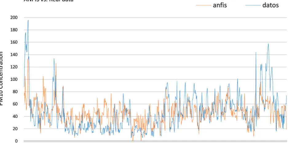
3. Results

To illustrate the complexity of the problem, the actual PM10 concentration data and its non-linear behavior can be observed in Figure 6.

For a better understanding about the complexity of the data it is necessary to analyze the variability of the data coming from the different monitoring stations. This variability has origin in the nature of the phenomenon of the behavior of the atmospheric particles, in Table 3 can be observed some measurements of dispersion of three stations, as a sample of this variability, we can see that the standard deviation shows that the data are distributed in a wider range.

Once the complexity of the problem is established, we can state that the pur-pose of using the BFOA optimization method is the reduction of the error that exists when applying the model created with ANFIS, which is why the experi-ments conducted are aimed at testing the efficiency of the BFO algorithm and the different configurations of its parameters.

It is important to calculate the error that is obtained when using ANFIS to create the model, which can be observed in Figure 7 and that, will later serve to

DOI: 10.4236/ijis.2019.93005 80 International Journal of Intelligence Science Figure 7. Error of ANFIS vs. real data.

Table 3. Variability of the data.

Station Minimum Maximum Range Standard deviation Mean

hgm 5 196 191 30.74678334 46.325452

fac 1 264 263 36.87219649 45.9357045

sag 3 238 235 34.85784066 58.5607094

cho 1 220 219 44.80596269 56.6182573

cua 1 168 167 27.56101595 33.4013699

cut 1 290 289 51.84183066 73.6511628

mgh 3 177 174 29.99927561 41.217862

make the comparison with the optimized model. The quantification of the error between the real data and those calculated by the ANFIS model was carried out using the root mean square error (RMSE) which is a method historically used to measure the accuracy of data forecasts [39].

The problem of using ANFIS to generate a pollutant concentration model is that the values obtained with ANFIS present large differences compared to the real values.

In the case of the model generated with ANFIS, an RMSE = 24,147 is ob-tained, which is expected to be minimized with BFOA.

DOI: 10.4236/ijis.2019.93005 81 International Journal of Intelligence Science

number of steps of chemotaxis and reproduction steps. However, the variation in BFOA parameters could generate a high execution time, given the nature of BFOA, since it is an algorithm that has nested cycles, that is why the processing time of each parameter configuration was also taken into account in the experi-ments.

Such experiments were focused on the parameter in question and in its effect on the model, that is why the other parameters were maintained fixed and on low values to avoid unnecessarily rising the execution time and avoid interfe-rence with the parameter tests.

As a context for the runtime tests, a PC with Windows 7, 64 bits, Intel Core i3-2100 3.10 GHz processor and 12 Gb RAM was used.

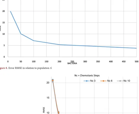
3.1. Variation in the Number of Bacteria

The number of bacteria in population S is perhaps the first parameter to choose, since each of the bacteria represents a possible solution to the optimization problem, even though it must be taken into account that increasing the size of S can also increase the computational complexity. However, if S has a large value and by randomly distributing the initial population in the search space, there is a greater probability that some of these bacteria have been positioned near an op-timal point, and that during the execution of the algorithm is also higher the probability that there is a higher density of bacteria in said optimal region.

The proposed values to experiment with the number of bacteria were S = {10, 50, 100, 200, 500}, in Table 4 it can be observed how the amount of bacteria in-fluences in obtaining an optimized model, achieving a lower error measurement (RMSE). However, it is important to note how the effect of the size of the popu-lation S in obtaining the error has a higher rate of change when the popupopu-lation is less than 50 and after that value the rate of change decreases (Figure 8). Howev-er, as the number of bacteria increases, so does the computational time as shown

on Table 4 up to the point to the time increasing considerably with a RMSE of

3.75, which is a decrease of only 1.57. For that reason, it is important to deter-mine the point where the number of bacteria shows a low RMSE, but the time does not increase considerably.

3.2. Variation of Chemotaxis Steps

When the steps of chemotaxis are increased, that is, Nc has a larger value, which

Table 4. Ratio of bacteria quantity, RMSE and execution time.

Bacteria RMSE Time/seconds

10 19.8851195 419.84

50 10.1072 2268.786

100 7.07398003 4185.117

200 5.32684396 8062.675

DOI: 10.4236/ijis.2019.93005 82 International Journal of Intelligence Science

results in a greater optimization advance when having more opportunities to reach an optimal point. Therefore, in Figure 9 we can observe a decrease in the error when Nc = 10 and especially when the population S is greater (S = 500), but this also implies a greater computational complexity. In addition, it can be noted on Figure 9 that the difference in RMSE then having 10 and 50 bacteria is negligible and a more consistent difference in RMSE is given between 200 and

Figure 8. Error RMSE in relation to population S.

DOI: 10.4236/ijis.2019.93005 83 International Journal of Intelligence Science

500 bacteria. Which seems to indicate that at low values the steps of which the bacteria moves does not have an effect on the results due that with few bacteria will take longer to find an optimum solution regardless of the steps.

3.3. Variation of Reproduction Steps

The reproduction steps, Nre, give an indication of how the algorithm ignores re-gions with few nutrients, and focuses on rere-gions with high nutritional content for the bacteria. This means, whether the bacteria are finding better solutions, given that the bacteria in bad regions die and bacteria that are in good regions tend to reproduce faster. Furthermore, if Nre is very small, the algorithm con-verges prematurely, and if on the contrary the value of the reproduction steps is very high, the computational complexity increases exponentially.

In Figure 10, the value of Nre and its corresponding RMSE is shown. In this

figure, is displayed that the RMSE decreases rapidly as the Nre increases up to 12. After this point, the optimization process no longer improves and the error begins to stall at a particular value, even if Nre increases up to 20.

In terms of computational complexity, in Figure 11 it can be observed that undoubtedly the complexity increases significantly when increasing the values of the reproduction steps where there is a considerable difference between the val-ues Nr = 12 and Nre = 20. This must be taken into account when selecting the parameters, since the improvement in the optimization is not significant in terms of but it does increase the complexity a lot.

3.4. Variation of the Elimination/Dispersion Events

The value of the elimination/dispersion events, Ned, refers to how many times a group of bacteria will be eliminated and new bacteria will be generated in ran-dom positions throughout the search space. This means that a low value for Ned will not have to rely on random elimination/dispersion events to find favorable regions, whilst a higher value of Ned will allow bacteria to have access to more

DOI: 10.4236/ijis.2019.93005 84 International Journal of Intelligence Science

regions of the search space in which they might find higher concentrations of nutrients. This parameter must be also being taken into account, that increasing the number of these events can increase computational complexity.

As a result of the tests carried out with different values for Ned, it can be seen

in Figure 12, that the Ned increase contributes to the result of obtaining a

smaller error in the optimized model. However, it can be seen in the same figure that by the time the population size is larger, Ned’s contribution is no longer as significant, since the error value for when Ned = 10 is very close to the error when Ned = 16. Due to the issues on computational complexity discussed pre-viously, it may be concluded that S = 50 and Ned = 10 may be the most appro-priate values to since S = 100 does not improve with a large value of Ned as shown on Figure 12 and in the values in Table 5.

Figure 11. Cost/Benefit of Nre in terms of execution time.

DOI: 10.4236/ijis.2019.93005 85 International Journal of Intelligence Science Table 5. Ned y RMSE values.

Ned S = 10 S = 100

2 21.9864716 8.53933847

4 14.1218685 2.93864778

10 7.00605537 1.12131925

16 4.17984705 1.18270545

3.5. Variation in Step Size Taken during the Tumble

C(i), where i=1,2, , S, is defined as the size of the step taken in a random di-rection specified by the tumble. One could say that C(i) is the size of the step by which the BFO algorithm advances. This makes it one of the main parameters to experiment in this contribution. However, it can be intuited that if the values of step C(i) are very large, and the optimum value is within a valley with very pro-nounced edges, the search could jump the valley without stopping, or it may also omit minimums locals swimming through them. On the other hand, if the values of C(i) are very small, the convergence becomes slower.

In Figure 13, an observation on how the value of C(i) when taking different

values affects the result obtained by the algorithm is seen. In this specific confi-guration its optimum value reaches with C(i) = 4 with an RMSE = 6.79, after that value, the error increases considerably. As explained above, this is due to the fact that the advance step of the algorithm, c(i), is directly linked to the nature of the problem since a very large value can skip regions with critical values (local or global minimums) and if is very small makes the convergence slower. C(i) = 4 is the best for the problem posed here.

For example, when C(i) = 30, the error is even greater than the one obtained with the non-optimized model, as expected, since the step is larger, it is easier to pass by regions with high nutrients if they are within a valley, thus avoiding local minimum.

3.6. Final Parameter Tuning

In the previous sections is explained the effect that have the most significant in obtaining the optimized model parameters and the individual effects that each of them have in the model. Based upon these results, it may be concluded that giv-en the appropriate configuration of the parameters are selected, the algorithm succeeds in reducing the Root Mean Square Error (RMSE) given a set of models for Airborne Particulate Matter PM10 without sacrificing computational speed.

The final configuration, proposed for the model optimized with BFO, is shown in Table 6.

In Figure 14, the error is shown for each hour of the month, corresponding to

DOI: 10.4236/ijis.2019.93005 86 International Journal of Intelligence Science Figure 13. Variation in step size taken during the tumble.

Figure 14. Comparison of errors of the ANFIS model and optimized model BFOA/ANFIS.

with BFOA, is better adjusted to the real data than the ANFIS method alone, in

Table 7, the errors calculated with RMSE, of each model for each of the different

values of the population S are presented.

DOI: 10.4236/ijis.2019.93005 87 International Journal of Intelligence Science Table 6. Final configuration of parameters.

Parameter Value

S 300

Nc 10

Ned 10

Nre 12

C(i) 4

Table 7. RMSE for ANFIS and BFOA.

S RMSE ANFIS RMSE BFOA

S = 10 25.1144672 4.62980105

S = 100 25.1144672 2.32101394

Figure 15. Comparison of errors of the optimized BFOA/ANFIS model with variation in population S.

BFOA, but with different sizes of population S, where it can be seen that the sig-nificant value is still the size of S, since we see that even errors of large scale (Figure 15, labeled 49.93).

4. Conclusions and Future Work

optimiza-DOI: 10.4236/ijis.2019.93005 88 International Journal of Intelligence Science

tion without increasing the execution time. Similarly, it was shown that, the size of the step, C(i), is an essential parameter, because its variation has a significant influence on the optimized model, and the range is narrow where the appropri-ate value is locappropri-ated. Apart from the parameters of chemotactic steps, Nc, and the number of reproduction steps, Nre also contributes to the final parameter con-figuration to obtain the optimized model.

Also, it is important to state that even though BFOA is a stochastic method and contains some degree of randomness, for instance, in the population gener-ation. That is why several tests must be performed to certainly know that the al-gorithm is reliable, along with the tests using validation data.

It should be mentioned that the implementation of the BFO algorithm was based on the author’s original version [20]. However, there is a very broad field where, as future research work, more data could be tested, for example, testing their performance with data from other cities around the world and even gene-rating an optimized model for PM2.5 particles. It could also include more mon-itoring stations, as well as the implementation of hybrid versions for this same application. For instance, the hybrid version of BFO with Optimization of Par-ticle Swarm (PSO) could be implemented as they have done in other works [40]. Also the hybrid version (HBFO) could be applied where a part of the ant colony optimization algorithm (ACO) is used in the rotation mechanism of artificial bacteria [28]. All of this is for obtaining better results in the modeling of conso-lidating BFOA as an optimization algorithm, and its successful application in a problem of environmental data.

Conflicts of Interest

The authors declare no conflicts of interest regarding the publication of this pa-per.

References

[1] Yang, X.S., Cui, Z., Xiao, R., Gandomi, A.H. and Karamanoglu, M. (2013) Swarm Intelligence and Bio-Inspired Computation: Theory and Applications.

[2] Health Effects Institute (2019) State of Global Air 2019. Special Report. Health Ef-fects Institute, Boston.

[3] Brunekreef, B. and Holgate, S.T. (2002) Air Pollution and Health. The Lancet, 360, 1233-1242.https://doi.org/10.1016/S0140-6736(02)11274-8

[4] Franklin, B.A., Brook, R. and Pope III, C.A. (2015) Air Pollution and Cardiovascu-lar Disease. Current Problems in Cardiology, 40, 207-238.

https://doi.org/10.1016/j.cpcardiol.2015.01.003

[5] Kurt, O.K., Zhang, J. and Pinkerton, K.E. (2016) Pulmonary Health Effects of Air Pollution. Current Opinion in Pulmonary Medicine, 22, 138.

https://doi.org/10.1097/MCP.0000000000000248

DOI: 10.4236/ijis.2019.93005 89 International Journal of Intelligence Science

[7] Cortina-Januchs, M.G., Quintanilla-Dominguez, J., Vega-Corona, A. and Andina, D. (2015) Development of a Model for Forecasting of PM10 Concentrations in Sa-lamanca, Mexico. Atmospheric Pollution Research, 6, 626-634.

https://doi.org/10.5094/APR.2015.071

[8] Moustris, K.P., Ziomas, I.C. and Paliatsos, A.G. (2010) 3-Day-Ahead Forecasting of Regional Pollution Index for the Pollutants NO2, CO, SO2, and O3 Using Artificial

Neural Networks in Athens, Greece. Water, Air and Soil Pollution, 209, 29-43. https://doi.org/10.1007/s11270-009-0179-5

[9] Alkasassbeh, M., Sheta, A.F., Faris, H. and Turabieh, H. (2013) Prediction of PM10 and TSP Air Pollution Parameters Using Artificial Neural Network Autoregressive, External Input Models: A Case Study in Salt, Jordan. Middle-East Journal of Scien-tific Research, 14, 999-1009.

[10] Zarandi, M., Faraji, M. and Karbasian, M. (2012) Interval Type-2 Fuzzy Expert Sys-tem for Prediction of Carbon Monoxide Concentration in Mega-Cities. Applied Soft Computing, 12, 291-301.https://doi.org/10.1016/j.asoc.2011.08.043

[11] Aceves-Fernandez, M.A., Estrada, A.L., Pedraza-Ortega, J.C., Gorrostieta-Hurtado, E. and Tovar-Arriaga, S. (2015) Design and Implementation of Ant Colony Algo-rithms to Enhance Airborne Pollution Models. International Journal of Environ-mental Science and Technology, 3, 22-28.

[12] Martinez-Zeron, E., Aceves-Fernandez, M.A., Gorrostieta-Hurtado, E., Soto-mayor-Olmedo, A. and Ramos-Arreguín, J.M. (2014) Method to Improve Airborne Pollution Forecasting by Using Ant Colony Optimization and Neuro-Fuzzy Algo-rithms. International Journal of Intelligence Science, 4, 81.

https://doi.org/10.4236/ijis.2014.44010

[13] Ordóñez-De León, B., Aceves-Fernandez, M.A., Fernandez-Fraga, S.M., Ra-mos-Arreguín, J.M. and Gorrostieta-Hurtado, E. (2019) An Improved Particle Swarm Optimization (PSO): Method to Enhance Modeling of Airborne Particulate Matter (PM10). Evolving Systems, 1-10.

https://doi.org/10.1007/s12530-019-09263-y

[14] Beni, G. and Wang, J. (1993) Swarm Intelligence in Cellular Robotic Systems. In:

Robots and Biological Systems: Towards a New Bionics, Springer, Berlin, Heidel-berg, 703-712.https://doi.org/10.1007/978-3-642-58069-7_38

[15] Dorigo, M., Maniezzo, V. and Colorni, A. (1996) Ant System: Optimization by a Colony of Cooperating Agents. IEEE Transactions on Systems, Man, and Cybernet-ics, Part B: Cybernetics, 26, 29-41.https://doi.org/10.1109/3477.484436

[16] Karaboga, D. (2005) An Idea Based on Honeybee Swarm for Numerical Optimiza-tion (Vol. 200). Technical Report tr06, Erciyes University, Engineering Faculty, Computer-Engineering Department, Kayseri.

[17] Hosseini, H.S. (2007) Problem Solving by Intelligent Water Drops. IEEE Congress on Evolutionary Computation, Singapore, 25-28 September 2007, 3226-3231. [18] Yang, X.S. (2010) A New Metaheuristic Bat-Inspired Algorithm. In: Nature Inspired

Cooperative Strategies for Optimization, Springer, Berlin, Heidelberg, 65-74. https://doi.org/10.1007/978-3-642-12538-6_6

[19] Hedayatzadeh, R., Salmassi, F.A., Keshtgari, M., Akbari, R. and Ziarati, K. (2010) Termite Colony Optimization: A Novel Approach for Optimizing Continuous Problems. 18th Iranian Conference on Electrical Engineering, Isfahan, 11-13 May 2010, 553-558.https://doi.org/10.1109/IRANIANCEE.2010.5507009

DOI: 10.4236/ijis.2019.93005 90 International Journal of Intelligence Science

https://doi.org/10.1109/MCS.2002.1004010

[21] Tripathy, M. and Mishra, S. (2007) Bacteria Foraging-Based Solution to Optimize Both Real Power Loss and Voltage Stability Limit. IEEE Transactions on Power Systems, 22, 240-248.https://doi.org/10.1109/TPWRS.2006.887968

[22] Das, S., Biswas, A., Dasgupta, S. and Abraham, A. (2009) Bacterial Foraging Opti-mization Algorithm: Theoretical Foundations, Analysis, and Applications. In:

Foundations of Computational Intelligence, Volume 3, Springer, Berlin, Heidelberg, 23-55.https://doi.org/10.1007/978-3-642-01085-9_2

[23] Ali, E.S. and Abd-Elazim, S.M. (2013) BFOA Based Design of PID Controller for Two Area Load Frequency Control with Nonlinearities. International Journal of Electrical Power & Energy Systems, 51, 224-231.

https://doi.org/10.1016/j.ijepes.2013.02.030

[24] Wu, C., Zhang, N., Jiang, J., Yang, J. and Liang, Y. (2007) Improved Bacterial Fo-raging Algorithms and Their Applications to Job Shop Scheduling Problems. In:

International Conference on Adaptive and Natural Computing Algorithms, Sprin-ger, Berlin, Heidelberg, 562-569.https://doi.org/10.1007/978-3-540-71618-1_62 [25] Mahapatra, G. and Banerjee, S. (2013) A Study of Bacterial Foraging Optimization

Algorithm and Its Applications to Solve Simultaneous Equations. International Journal of Computer Applications, 72, 1-6.https://doi.org/10.5120/12487-7927 [26] Chen, Y.P., Li, Y., Wang, G., Zheng, Y.F., Xu, Q., Fan, J.H. and Cui, X.T. (2017) A

Novel Bacterial Foraging Optimization Algorithm for Feature Selection. Expert Systems with Applications, 83, 1-17.https://doi.org/10.1016/j.eswa.2017.04.019 [27] Narendhar, S. and Amudha, T. (2012) A Hybrid Bacterial Foraging Algorithm for

Solving Job Shop Scheduling Problems.

[28] Abd-Elazim, S.M. and Ali, E.S. (2013) A Hybrid Particle Swarm Optimization and Bacterial Foraging for Optimal Power System Stabilizers Design. International Journal of Electrical Power & Energy Systems, 46, 334-341.

https://doi.org/10.1016/j.ijepes.2012.10.047

[29] Azizipanah-Abarghooee, R. (2013) A New Hybrid Bacterial Foraging and Simplified Swarm Optimization Algorithm for Practical Optimal Dynamic Load Dispatch. In-ternational Journal of Electrical Power & Energy Systems, 49, 414-429.

https://doi.org/10.1016/j.ijepes.2013.01.013

[30] Sistema de Monitoreo Atmosférico (SIMAT) El monitoreo de la calidad del aire. http://www.aire.cdmx.gob.mx/default.php?opc=%27ZaBhnmI=%27

[31] Red de Meteorología y Radiación Solar, REDMET.

http://www.aire.cdmx.gob.mx/default.php?opc=%27aKBi%27

[32] Angelov, P. (1994) A Generalized Approach to Fuzzy Optimization. International Journal of Intelligent Systems, 9, 261-268. https://doi.org/10.1002/int.4550090302 [33] Angelov, P., Sadeghi-Tehran, P. and Ramezani, R. (2011) An Approach to

Auto-matic Real-Time Novelty Detection, Object Identification, and Tracking in Video Streams Based on Recursive Density Estimation and Evolving Takagi-Sugeno Fuzzy Systems. International Journal of Intelligent Systems, 26, 189-205.

https://doi.org/10.1002/int.20462

[34] Jang, J.S. (1993) ANFIS: Adaptive-Network-Based Fuzzy Inference System. IEEE Transactions on Systems, Man, and Cybernetics, 23, 665-685.

https://doi.org/10.1109/21.256541

[35] Angelov, P. and Kasabov, N. (2005) Evolving Computational Intelligence Systems.

DOI: 10.4236/ijis.2019.93005 91 International Journal of Intelligence Science

17-19 March 2005, 76-82.

[36] Abdulshahed, A.M., Longstaff, A.P. and Fletcher, S. (2015) The Application of ANFIS Prediction Models for Thermal Error Compensation on CNC Machine Tools. Applied Soft Computing, 27, 158-168.

https://doi.org/10.1016/j.asoc.2014.11.012

[37] Hansen, C.H., Endres, R.G. and Wingreen, N.S. (2008) Chemotaxis in Escherichia coli: A Molecular Model for Robust Precise Adaptation. PLoS Computational Biol-ogy, 4, e1.https://doi.org/10.1371/journal.pcbi.0040001

[38] Brabazon, A. and McGarraghy, S. (2018) Foraging-Inspired Optimization Algo-rithms. Springer, Berlin.https://doi.org/10.1007/978-3-319-59156-8

[39] Hyndman, R.J. and Koehler, A.B. (2006) Another Look at Measures of Forecast Accuracy. International Journal of Forecasting, 22, 679-688.

https://doi.org/10.1016/j.ijforecast.2006.03.001

[40] Panda, S., Mohanty, B. and Hota, P.K. (2013) Hybrid BFOA-PSO Algorithm for Automatic Generation Control of Linear and Nonlinear Interconnected Power Sys-tems. Applied Soft Computing, 13, 4718-4730.