Type 1 and interval type 2 ANFIS: a comparison

Type-1 and Interval Type-2 ANFIS: A Comparison

Chao Chen, Robert John, Jamie Twycross, Jonathan M. Garibaldi

University of Nottingham

Email:{chao.chen, robert.john, jamie.twycross, jon.garibaldi}@nottingham.ac.uk

Abstract—In a previous paper, we proposed an extended

ANFIS architecture and showed that interval type-2 ANFIS produced larger errors than type-1 ANFIS on the well-known IRIS classification problem. In this paper, more experiments on both synthetic and real-world data are conducted to further investigate and compare the performance of interval type-2 ANFIS and type-1 ANFIS. For each dataset, interval type-2 ANFIS is optimised in three different ways, including a strategy suggested by Mendel such that interval type-2 ANFIS would be no worse than type-1 ANFIS. Our results show that in some circumstances the performance of interval type-2 ANFIS can be improved when it is initialised with blurred optimised type-1 ANFIS parameters. However, in general, interval type-2 ANFIS does not produce a clear performance improvement compared to type-1 ANFIS, especially on Mackey-Glass data with large noise. Thus, we conclude that the choice of interval type-2 ANFIS over type-1 ANFIS should be carefully considered, since type-2 ANFIS is more computationally complex, yet significantly better performance cannot be easily obtained.

I. INTRODUCTION

Since its introduction by Zadeh in 1965 [1], fuzzy logic has become more and more popular. Due to its capability in dealing with uncertainty, fuzzy logic system (FLS) has been shown to have many advantages in modelling applications in many areas including engineering, natural science, and time series forecasting [2, 3, 4].

Up until the beginning of this century, there was a heavy emphasis on type-1 (T1) FLS. During the past few years, there has been a steady increase of interest in type-2 (T2) FLS, especially in interval type-2 (IT2) FLS [5], and a number of works have helped to make the implementation of T2 FLS straightforward [6, 7]. Furthermore, it has been demonstrated that in principle T2 FLS is able to provide better (and certainly no worse) performance than T1 FLS [8]. This can be guaranteed by initialising the membership functions of an IT2 FLS with the membership functions of an optimised T1 FLS. However, in practice, it should be noted that IT2 FLS does not always provide significant improvement compared to T1 FLS. In fact, IT2 FLS can in some cases be worse than T1 FLS if they are both optimised from scratch [9].

The Adaptive-Network-based Fuzzy Inference System (AN-FIS) was proposed by Jang [10] to serve as a basis for constructing a set of fuzzy rules with appropriate membership functions to generate the required fuzzy inference system. In many studies, ANFIS has been shown to be superior to models using other techniques such as autoregression, genetic algorithms and artificial neural networks [11, 12, 13]. An increasing interest in T2 FLS has also led to an increase in the

research on IT2 ANFIS. Early studies can be found in [14, 15] which described an approach that uses an adaptive network to learn a T2 fuzzy system based on linguistic inputs and numeric output.

Very few comparisons have been made between the perfor-mance of T1 and IT2 ANFIS models, especially on accessible or reproducible datasets. In a previous study [9], we have shown that the least-square-estimate (LSE) method together with the Karnik-Mendel (KM) algorithm behaves differently for interval IT2 ANFIS compared to T1 ANFIS. And in that paper, IT2 ANFIS produced generally larger root-mean-squared-error (RMSE) than T1 ANFIS on the well-known IRIS classification problem.

In this paper, we further investigate the performance differ-ences between T1 and IT2 ANFIS models on both synthetic and real-world data. Moreover, as suggested in [8], IT2 ANFIS models are also optimised from two different types of opti-mised T1 ANFIS membership functions. We also compare our results to a na¨ıve method and two commonly used algorithms (linear regression and support-vector-machines) as the baseline of desired performance.

The remainder of this paper is organised as follows: Sec-tion II introduces the optimisaSec-tion methods and corresponding notations for ANFIS models used in this paper; In Section III, experiments evaluating model performance on both synthetic and real-world data are described. The results of these exper-iments are discussed in Section IV. Finally, conclusions and suggestions for the future work are given in Section V.

II. ANFIS OPTIMISATION

In this paper, the architecture of T1 and IT2 ANFIS models is based on the work in [9]. Specifically, the antecedent membership functions of our T1 ANFIS models are based on the generalised bell-shaped function defined as:

μ = 1

1 + (x−c a )2b

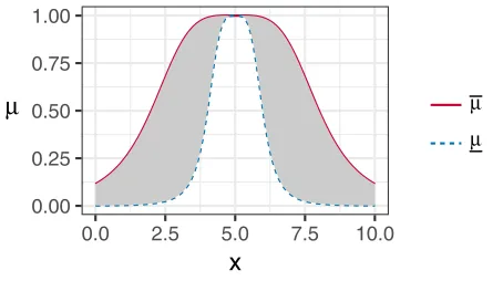
wherexis the crisp input and{a, b, c}are real-valued param-eters, a, b > 0. Similarly, the lower and upper membership functions for IT2 ANFIS are also based on generalised bell-shaped functions (see Fig. 1 as an example), defined as:

¯

μ ₌ 1

1 + (x−c

¯ a )2b ¯

μ ₌ 1

1 + (x−c

where { ¯

a_{,¯a, b, c} are real-valued parameters, ¯a >} ¯ a_, ¯

a_{, b>0. The consequent membership functions for both T1}

0.00 0.25 0.50 0.75 1.00

0.0 2.5 5.0 7.5 10.0

x

μ

μ

Fig. 1: An illustration of the IT2 membership function where {a_{= 1,¯a= 3, b= 2, c = 5}.}

and IT2 ANFIS are the same. They are based on first-order linear function f_i (for the ith rule), as defined below (for a model with two inputs x₁ andx₂):

fi=pi+qix1+rix2 wherep_i, q_i, r_i are the coefficients.

Before optimisation, all parameters of T1 and IT2 models are given initial values in different ways. Different notations are used in this paper in order to summarise how they are ini-tialised. Specifically, all T1 ANFIS models are initialised from scratch and it is summarised as AT1-SCRATCH. IT2 ANFIS models are initialised in three different ways: (i), similar to T1 ANFIS, all IT2 membership functions are initialised from scratch (AT2-SCRATCH); (ii), IT2 membership functions are initialised with optimised T1 membership functions (AT2-OPT). Specifically, the upper and lower membership functions

¯

μ _{andμ¯are set to be the same as corresponding T1} member-ship functionμ; iii), IT2 membership functions are initialised by blurring optimised T1 membership functions (AT2-BLUR). Specifically,

¯a= 0.9a,¯a= 1.1a,b =b andc =c.

In this paper, both T1 and IT2 ANFIS models are optimised by the hybrid learning algorithms based on back-propagation and the LSE algorithm. The training process for optimising T1/IT2 ANFIS models is described as follows:

1) Build and initialise the T1/IT2 modelanfiswith arbitrar-ily or specified antecedent and consequent parameters. 2) Set the optimised error e = ∞ and the optimised

(output) modelanfis=anfis.

3) Loop the following sub-steps (training epoch) until e equals to zero or it reaches the maximum training epochs defined (500 epochs in this paper):

a) If the model is optimised by solely back-propagation approach, goto Step 3d.

b) In the forward pass, estimate the consequent pa-rameters by the LSE algorithm with training data. c) Update anfis with the estimated consequent

pa-rameters.

d) Evaluate the updated model anfis with validation data to obtain the corresponding validation errore

(If there are no validation data, then use training data instead in this step.).

e) Ife< e, sete=e andanfis=anfis.

f) In the back propagation process, update the an-tecedent parameters ofanfisby the gradient decent method. If required, the consequent parameters can also be updated by the gradient decent method. 4) Setanfis as the output of the optimisation process.

III. EVALUATION

To make comparisons between T1 and IT2 ANFIS modes, both synthetic and real-world data are used. Specifically, the well-known MG equation is used to generate synthetic data. For the real-world data, two widely used benchmark problems in the fuzzy logic community are used: the estimation of the low voltage electrical line length and the estimation of the medium voltage electrical line maintenance cost in towns.

Comparisons have also been made with a simple method and two commonly used algorithms: linear regression (LR) and support-vector-machines (SVM). The LR and SVM models are implemented with built-in R functions using default parame-ters. Results from literature are also presented for comparisons. The simple method used in this paper is described as fol-lows: (i) From all the input variables of the training data, select a single input variable x_i which has the highest correlation with the output y; (ii) For all the entries of the training data, calculate the median of the ratio y/x_i as the constant coefficient p; (iii) use px_i as the prediction. Basically, for the MG data, this simple method is doing similar to the na¨ıve method [16], which uses the last available value as the prediction. Thus, we call it na¨ıve method in this paper.

A. Mackey-Glass time series prediction

1) Mackey-Glass time series: The settings to generate MG time series in this paper are selected from the literature [10, 17, 18]. Specifically, the fourth-order Runge-Kutta method is used and the initial settings are: time step = 0.1; x(0) = 1.2 and x(t) = 0 fort <0;τ= 17. x(t) is thus derived for0t1200. In this paper, both noiseless and noisy MG data are used. For the noisy MG series, five different signal-to-noise ratios are used. They are 0dB, 10dB, 20dB, 30dB and 40dB respectively. The well-known formula in [19] for the signal-to-noise ratio (SNR) is:

SNR= 10 log₁₀

σ2 s σ2 n

whereσ_sis the standard deviation of the signal andσ_n is the the standard deviation of the noise.

2) Input-output data pairs: 1000 input-output data pairs are extracted from the above series for t = 118 to 1117. For each t, x(t-18), x(t-12), x(t-6) and x(t) are used as inputs and x(t+6) is the single output. The first 500 data pairs are used as training set, and remaining 500 data pairs are used as testing set.

0dB 10dB 20dB 30dB 40dB Noisy-free

SD(mg) 0.2267 0.2267 0.2267 0.2267 0.2267 0.2267

SD(noise) 0.2391 0.0756 0.0239 0.0076 0.0024 −

SD(series) 0.3233 0.2363 0.2271 0.2266 0.2266 0.2267

T1-ANFIS(Jang) −/− −/− −/− −/− −/− 0.0016/0.0015

T1-ANFIS(Castro) −/0.2910 −/0.1031 −/0.0333 −/0.0115 −/− −/0.0070

T1-SA(Almaraashi) −/0.3273 −/0.1549 −/0.0777 −/0.0352 −/0.2031 −/0.0090

na¨ıve 0.3803/0.3661 0.2090/0.2115 0.1882/0.1903 0.1858/0.1865 0.1860/0.1862 0.1858/0.1857 LR 0.2852/0.2841 0.1345/0.1352 0.1002/0.1014 0.0968/0.0967 0.0970/0.0962 0.0972/0.0962

SVM 0.2644/0.2888 0.0965/0.0981 0.0338/0.0343 0.0152/0.0149 0.0132/0.0128 0.0139/0.0134

AT1-SCRATCH 0.2527/0.3600 0.0892/0.1150 0.0301/0.0376 0.0107/0.0126 0.0040/0.0046 0.0016/0.0015 AT2-SCRATCH 0.2417/0.3357 0.0881/0.1118 0.0298/0.0366 0.0106/0.0131 0.0041/0.0048 0.0020/0.0019 AT2-OPT 0.2492/0.3427 0.0887/0.1139 0.0298/0.0393 0.0106/0.0128 0.0039/0.0045 0.0015/0.0014 AT2-BLUR 0.2485/0.3426 0.0872/0.1201 0.0296/0.0419 0.0104/0.0131 0.0039/0.0046 0.0015/0.0014

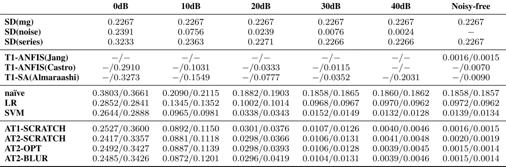
TABLE I: Training/Testing RMSE by different Models for predicting the MG series with different noise.

4) Results: The RMSE on training and testing data are shown in Table I. Key results from the literature [10, 17, 18] are also presented. To provide more insight of the comparisons, the standard deviations of both the MG series and the added noise are also shown in the table. Specifically, SD(mg) is the standard deviation of the MG series without noise. SD(noise) is the standard deviation of the added noise. SD(series) is the standard deviation of the MG series with added noise.

B. Low voltage electrical line length estimation

The measurement of electricity line length is useful for many aspects such as the maintenance costs of the network. Compared to the measurement of high and medium voltage lines, low voltage lines, which are normally distributed in cities and villages, are more difficult to be measured directly. Therefore, an indirect method for determining the length of low voltage lines is required. In this section, T1 and IT2 fuzzy models are built to estimate the total length of low voltage line installed in a rural town.

1) Data: The data set used in this section can be obtained from http://decsai.ugr.es/∼casillas/fmlib/ele1-2-495. html. There are 495 samples in the data set. Each sample has three attributes, where the first two are inputs and the other one is the output. Specifically, the inputs are the number of inhabitants in the town and the mean of the distances from the center of the town to the three furthest clients in it. The output is the total length of low voltage line installed in the town. Five example samples of the data set are presented in Table II. The original data set was randomly divided into five different subsets, with 99 samples in each subset [20]. By joining four of these subsets in a training data set and keeping the fifth subset as test data set, five different partitions has been built at the ratio of 80% to 20% to serve as the training and testing data respectively [21]. In this paper, five-fold cross-validation is applied for all ANFIS models with all the five data partitions provided on the website.

2) ANFIS modelling: All T1 and IT2 ANFIS models here have 2 inputs (2 membership functions for each input), 1

Inhabitants Distance to Clients Length of Low Voltage Line

10 648.330017 1773

32 383.329987 1104

4 126.669998 392

36 776.669983 2087

34 343.329987 1224

TABLE II: Five example data samples for the problem of low voltage electrical line length estimation

Street Length Area of Town Building Area Energy Supply Maintenance costs 11.00 3.30 54.959999 55.00 4329.330078

4.00 1.20 19.980000 40.00 2016.439941 0.90 0.27 4.500000 1.80 249.419998 2.00 1.20 19.980000 10.00 1044.219971 2.00 1.80 19.980000 30.00 1761.920044

TABLE III: Five example data samples for the problem of medium voltage electrical line maintenance cost estimation.

output and 4 rules.

3) Results: The RMSE on training and testing data are shown in Table IV. The best cross-validation results (referred to as COR [21]) on the data website and the key results (referred to as HA-PAES-MG-K_max) from the recent liter-ature [22] are also presented in the table. Note that results from the literature were MSE and they have been converted to RMSE in this paper.

C. Medium voltage electrical line maintenance cost estimation This problem involves the estimation of the minimum maintenance costs which are based on a model of the optimal electrical network for Spanish towns. It was originally pro-posed in [23]. In this problem, there are four input variables, which are the sum of the lengths of all streets in the town, the total area of the town, the area that is occupied by buildings, and the energy supply to the town.

The whole data set has been randomly divided into 5 different subsets (four of them with 211 samples and one of them with 212 samples). By joining four of these subsets in a training data set and keeping the fifth subset as test data set, five different partitions has been built at the ratio of 80% to20% to serve as the training and testing data respectively [21]. In this paper, five-fold cross-validation is applied. Thus, all the five data partitions provided on the website are used.

2) ANFIS modelling: All T1 and IT2 ANFIS models here have 4 inputs (2 membership functions for each input), 1 output and 16 rules.

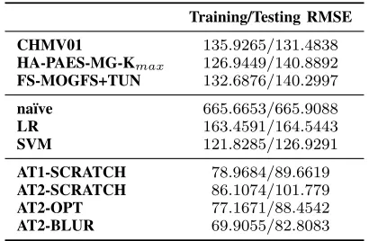
3) Results: The RMSE on training and testing data are shown in Table V. The best results listed on the data website (referred to as CHMV01 [24]) and the best results (referred to as HA-PAES-MG-K_max and FS-MOGFS+TUN) from the recent literature [22, 25] are also presented in the table. Note that results from the literature were MSE and they have been converted to RMSE in this paper.

Training/Testing RMSE

COR 585.9334/637.2598

HA-PAES-MG-K_max 532.2894/619.7451

na¨ıve 739.0226/736.6744

LR 631.2659/644.4992

SVM 582.3314/625.9389

AT1-SCRATCH 562.3696/703.8635 AT2-SCRATCH 570.7734/759.0388 AT2-OPT 562.3460/702.8623 AT2-BLUR 566.5998/794.1014

TABLE IV: Training/Testing RMSE on low voltage elec-tricity data (5-fold cross-validation).

Training/Testing RMSE

CHMV01 135.9265/131.4838

HA-PAES-MG-Kmax 126.9449/140.8892

FS-MOGFS+TUN 132.6876/140.2997

na¨ıve 665.6653/665.9088

LR 163.4591/164.5443

SVM 121.8285/126.9291

AT1-SCRATCH 78.9684/89.6619

AT2-SCRATCH 86.1074/101.779

AT2-OPT 77.1671/88.4542

AT2-BLUR 69.9055/82.8083

TABLE V: Training/Testing RMSE on medium voltage electricity data (5-fold cross-validation).

D. Statistical comparison

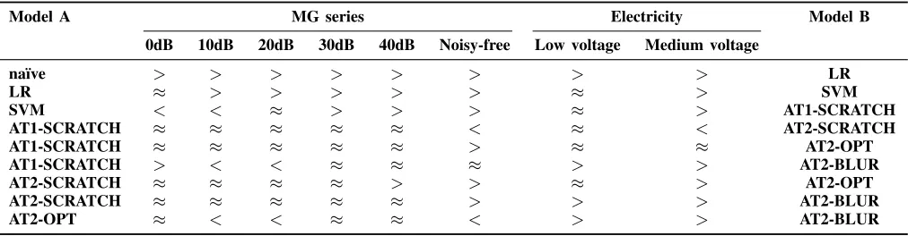
Statistical comparisons of the RMSE by different models have been made based on the Wilcoxon signed rank test, which is a non-parametric statistical hypothesis test. The significance level is 0.05. Results are shown in Tables VI and VII.

IV. DISCUSSION

As can be observed in Tables I, IV and V, AT2-SCRATCH models, for which IT2 membership functions were initialised

from scratch, produced mostly larger RMSE than AT1-SCRATCH models. Specifically, on the low and medium voltage electricity data, all the training and testing RMSE values of AT2-SCRATCH models are larger than those of AT1-SCRATCH. This behaviour is consistent with that described in [9].

It has been discussed in [8] that IT2 FLS can be guaranteed to be no worse than T1 FLS by initialising IT2 FLS with optimised T1 FLS. However, it has to be mentioned that this guarantee is only valid for training or validation data. Note that testing data are always unknown and a model can never be guaranteed to fit the testing data as well as it fitted the training or validation data. As can be seen in Tables I ,IV and V, all the training RMSE by AT2-OPT models are no larger than the training RMSE by AT1-SCRATCH. However, some testing RMSE of AT2-OPT models are larger than corresponding RMSE of AT1-SCRATCH. Also, it is found that even for the training RMSE, AT2-OPT does not provide a clear perfor-mance improvement especially for the low voltage electricity data. This may be because T1 ANFIS has reached a local optimum and optimising IT2 ANFIS starting from this local optimum may get stuck.

To address such local optimum issue, AT2-BLUR models are initialised from blurred optimised T1 ANFIS membership functions. Though BLUR models perform similar to AT2-OPT models for MG series and the low voltage data, it can be observed in Table V that AT2-BLUR models produced clearly smaller RMSE than other models. This behaviour is encouraging and it needs to be further investigated with more data to figure out in which circumstances AT2-BLUR models are better. On the other hand, we have only tried one simple method to blur T1 membership functions for generating IT2 membership functions. In future work, it would be interesting to investigate the effect of different blurring methods.

Another interesting point is that our ANFIS models pro-duced much better results (about 40% smaller RMSE) on the medium voltage electricity data than the best results reported in the literature. The results of our models on other datasets are also competitive. As can be concluded in Tables VI and VII, T1 ANFIS are significantly better than SVM and LR. This indicates that ANFIS is a very good approach and it is worth more attention and investigations for its remarkable ability.

Further more, Tables VI and VII show that there is no significant difference between T1 and IT2 ANFIS models on most of our comparisons. This is particularly clear on MG data with large noise, and on the low electricity data. It is also found that on these data, all the methods including the na¨ıve method produce similar results. Hence, it may indicate that on such data there would be no benefit for using IT2 ANFIS.

Model A MG Series Electricity Model B

0dB 10dB 20dB 30dB 40dB Noisy-free Low voltage Medium voltage

na¨ıve > > > > > > > > LR

LR > > > > > > > > SVM

SVM ≈ > > > > > < > AT1-SCRATCH

AT1-SCRATCH > ≈ ≈ ≈ ≈ < ≈ < AT2-SCRATCH

AT1-SCRATCH ≈ ≈ ≈ ≈ ≈ > > < AT2-OPT

AT1-SCRATCH ≈ ≈ ≈ ≈ ≈ ≈ ≈ > AT2-BLUR

AT2-SCRATCH ≈ ≈ ≈ ≈ ≈ > ≈ > AT2-OPT

AT2-SCRATCH ≈ ≈ ≈ ≈ ≈ > ≈ > AT2-BLUR

AT2-OPT ≈ ≈ ≈ ≈ ≈ ≈ ≈ > AT2-BLUR

TABLE VI: Statistical comparisons of models (A and B) on training RMSE based on the Wilcoxon signed rank test at 0.05 significance level, where>means statistically larger,<means statistically smaller and≈means no significant difference.

Model A MG series Electricity Model B

0dB 10dB 20dB 30dB 40dB Noisy-free Low voltage Medium voltage

na¨ıve > > > > > > > > LR

LR ≈ > > > > > ≈ > SVM

SVM < < ≈ > > > ≈ > AT1-SCRATCH

AT1-SCRATCH ≈ ≈ ≈ ≈ ≈ < ≈ < AT2-SCRATCH

AT1-SCRATCH ≈ ≈ ≈ ≈ ≈ > ≈ ≈ AT2-OPT

AT1-SCRATCH > < < ≈ ≈ ≈ > > AT2-BLUR

AT2-SCRATCH ≈ ≈ ≈ ≈ > > ≈ > AT2-OPT

AT2-SCRATCH ≈ ≈ ≈ ≈ ≈ > > > AT2-BLUR

AT2-OPT ≈ < < ≈ ≈ < > > AT2-BLUR

TABLE VII: Statistical comparisons of models (A and B) on testing RMSE based on the Wilcoxon signed rank test at 0.05 significance level, where>means statistically larger,<means statistically smaller and≈means no significant difference.

and SVM models. However, in contrast, the training RMSE for the model AT1-SCRATCH was smaller than LR and SVM models. This seems to be an over-fitting problem. Note that in this paper, datasets were divided into only training and testing sets so that our results can be compared with literature. Normally, the over-fitting issue can be addressed by using validation set during the training process.

Though testing errors are more important than training errors, it is arguably that in some circumstances training errors can also indicate the potential capability of a model. In Table I, all the training errors of our ANFIS models are smaller than other models. And in fact, they are very close to the standard deviation of the added noise. Note that it is an intuition that random noise cannot be predicted. In other words, the smallest RMSE of a model predicting something with random noise should be roughly equal to the standard deviation of the random noise. This provides some indication that ANFIS models may be able to provide better testing performance if the over-fitting issue can be sufficiently addressed.

In conclusion, though IT2 ANFIS might be expected to be better as it has more model parameters than T1 ANFIS, we have shown that this is not always the case, and it is not easy to optimise IT2 ANFIS from scratch. Thus, the use of IT2 ANFIS should be carefully considered since it may not bring a clear performance improvement compared to T1

ANFIS. On the other hand, initialising IT2 ANFIS based on an optimised T1 ANFIS could help in optimising IT2 ANFIS. In particular, it is suggested to initialise IT2 ANFIS based on blurred membership functions of an optimised T1 ANFIS. It should be noted that even based on the above strategy, IT2 ANFIS in some circumstances may not be able to provide a clear performance improvement compared to T1 ANFIS. We do not suggest to use IT2 ANFIS on datasets with large noise when a sophisticated algorithm (e.g. LR or SVM) does not provide clearly better performance than a relatively simple method (e.g. the na¨ıve method).

V. CONCLUSION

should be initialised based on blurred membership functions of an optimised T1 ANFIS. We have shown that ANFIS models were very competitive compared to other commonly used models such as LR and SVM. In the future, it would be interesting to try more variations of the initialisation method for IT2 ANFIS based on an optimised T1 ANFIS. It would also be interesting to see comparisons of T1 and IT2 ANFIS, as well as other methods such as LR and SVM, in both accuracy and time efficiency with larger datasets.

REFERENCES

[1] L. A. Zadeh, “Fuzzy sets,” Information and Control, vol. 8, no. 3, pp. 338–353, 1965.

[2] O. Castillo and P. Melin, “A review on the design and optimization of interval type-2 fuzzy controllers,” Applied Soft Computing, vol. 12, no. 4, pp. 1267–1278, 2012.

[3] D. Soria, J. M. Garibaldi, A. R. Green, D. G. Powe, C. C. Nolan, C. Lemetre, G. R. Ball, and I. O. Ellis, “A quantifier-based fuzzy classification system for breast cancer patients.” Artificial Intelligence in Medicine, vol. 58, no. 3, pp. 175–84, 2013.

[4] A. Pourabdollah, C. Wagner, J. H. Aladi, and J. M. Garibaldi, “Improved Uncertainty Capture for Nonsin-gleton Fuzzy Systems,” IEEE Transactions on Fuzzy Systems, vol. 24, no. 6, pp. 1513–1524, 2016.

[5] J. Mendel, H. Hagras, W.-W. Tan, W. W. Melek, and H. Ying, Introduction To Type-2 Fuzzy Logic Control: Theory and Applications, 1st ed. Wiley-IEEE Press, 2014.

[6] J. M. Mendel, R. I. John, and F. Liu, “Interval Type-2 Fuzzy Logic Systems Made Simple,”IEEE Transactions on Fuzzy Systems, vol. 14, no. 6, pp. 808–821, 2006. [7] D. Wu and J. M. Mendel, “Designing practical interval

type-2 fuzzy logic systems made simple,” inProceedings IEEE International Conference on Fuzzy Systems, 2014, pp. 800–807.

[8] J. M. Mendel, “General type-2 fuzzy logic systems made simple: a tutorial,”IEEE Transactions on Fuzzy Systems, vol. 22, no. 5, pp. 1162–1182, 2014.

[9] C. Chen, R. John, J. Twycross, and J. M. Garibaldi, “An extended ANFIS architecture and its learning properties for type-1 and interval type-2 models,” in Proceedings IEEE International Conference on Fuzzy Systems, 2016, pp. 602–609.

[10] J.-S. Jang, “ANFIS: adaptive-network-based fuzzy infer-ence system,”IEEE Transactions on Systems, Man, and Cybernetics, vol. 23, no. 3, pp. 665–685, 1993.

[11] A. Azadeh, M. Saberi, A. Gitiforouz, and Z. Saberi, “A hybrid simulation-adaptive network based fuzzy infer-ence system for improvement of electricity consumption estimation,” Expert Systems with Applications, vol. 36, no. 8, pp. 11 108–11 117, 2009.

[12] L.-Y. Wei, T.-L. Chen, and T.-H. Ho, “A hybrid model based on adaptive-network-based fuzzy inference system

to forecast Taiwan stock market,” Expert Systems with Applications, vol. 38, no. 11, pp. 13 625–13 631, 2011. [13] A. K. Lohani, R. Kumar, and R. D. Singh,

“Hydro-logical time series modeling: A comparison between adaptive neuro-fuzzy, neural network and autoregressive techniques,”Journal of Hydrology, vol. 442-443, pp. 23– 35, 2012.

[14] R. I. John and C. Czarnecki, “A type 2 adaptive fuzzy inferencing system,” in Proceedings IEEE International Conference on Systems, Man, and Cybernetics, vol. 2, 1998, pp. 2068–2073.

[15] R. I. John and C. Czarnecki, “An adaptive type-2 fuzzy system for learning linguistic membership grades,” in Proceedings IEEE International Conference on Fuzzy Systems, vol. 3, 1999, pp. 1552–1556.

[16] S. Makridakis and M. Hibon, “The M3-Competition: re-sults, conclusions and implications,” International Jour-nal of Forecasting, vol. 16, no. 4, pp. 451–476, 2000. [17] J. R. Castro, O. Castillo, P. Melin, and A.

Rodr´ıguez-D´ıaz, “A hybrid learning algorithm for a class of interval type-2 fuzzy neural networks,”Information Sciences, vol. 179, no. 13, pp. 2175–2193, 2009.

[18] M. Almaraashi and R. John, “Tuning fuzzy systems by simulated annealing to predict time series with added noise,” in proceedings UK Workshop on Computational Intelligence, 2010, pp. 1–5.

[19] J. Mendel, Uncertain Rule-Based Fuzzy Logic Systems: Introduction and New Directions. Prentice Hall, 2001. [20] O. Cordon, F. Herrera, and P. Villar, “Generating the knowledge base of a fuzzy rule-based system by the genetic learning of the data base,” IEEE Transactions on Fuzzy Systems, vol. 9, no. 4, pp. 667–674, 2001. [21] J. Casillas, O. Cordon, and F. Herrera, “COR: a

method-ology to improve ad hoc data-driven linguistic rule learning methods by inducing cooperation among rules,” IEEE Transactions on Systems, Man, and Cybernetics, Part B (Cybernetics), vol. 32, no. 4, pp. 526–537, 2002. [22] C. H. Nguyen, V. T. Hoang, and V. L. Nguyen, “A discussion on interpretability of linguistic rule based systems and its application to solve regression problems,” Knowledge-Based Systems, vol. 88, pp. 107–133, 2015. [23] O. Cord´on, F. Herrera, and L. S´anchez, “Solving

Elec-trical Distribution Problems Using Hybrid Evolutionary Data Analysis Techniques,”Applied Intelligence, vol. 10, no. 1, pp. 5–24, 1999.

[24] O. Cord´on, F. Herrera, L. Magdalena, and P. Villar, “A genetic learning process for the scaling factors, granu-larity and contexts of the fuzzy rule-based system data base,” Information Sciences, vol. 136, no. 1-4, pp. 85– 107, 2001.