MORPHODYNAMIC PATTERNS FROM
2DEPTH-AVERAGED SEDIMENT
3CONCENTRATION
4F. Ribas1, A. Falqu´es1, H.E. de Swart2, N. Dodd3, R. Garnier4, and D. Calvete1
5
Corresponding author: F. Ribas, Department of Applied Physics, Universitat Polit`ecnica de
Catalunya, Barcelona, Spain. ([email protected])
1Department of Applied Physics, Universitat Polit`ecnica de Catalunya, Barcelona, Spain
2Institute for Marine and Atmospheric research, Utrecht University, Utrecht, the Netherlands
3Faculty of Engineering, University of Nottingham, Nottingham, UK
This review highlights the important role of the depth-averaged sediment concen-6
tration (DASC) to understand the formation of a number of coastal morphodynamic 7
features that have an alongshore rhythmic pattern: beach cusps, surf zone transverse 8
and crescentic bars, and shoreface-connected sand ridges. We present a formulation 9
and methodology, based on the knowledge of the DASC (which equals the sediment 10
load divided by the water depth), that has been successfully used to understand the 11
characteristics of these features. These sand bodies, relevant for coastal engineering 12
and other disciplines, are located in different parts of the coastal zone and are char-13
acterized by different spatial and temporal scales, but the same technique can be 14
used to understand them. Since the sand bodies occur in the presence of depth-averaged 15
currents, the sediment transport approximately equals a sediment load times the cur-16
rent. Moreover, it is assumed that waves essentially mobilize the sediment and the 17
current increases this mobilization and advects the sediment. In such conditions, know-18
ing the spatial distribution of the DASC and the depth-averaged currents induced 19
by the forcing (waves, wind, and pressure gradients) over the patterns allows infer-20
ring the convergence/divergence of sediment transport. Deposition (erosion) occurs 21
where the current flows from areas of high to low (low to high) values of DASC. The 22
formulation and methodology are especially useful to understand the positive feed-23
back mechanisms between flow and morphology leading to the formation of those 24
morphological features, but the physical mechanisms for their migration, their finite-25
1. INTRODUCTION
Coastal zones are highly valued worldwide for their natural beauty, the recreational 27
opportunities they offer and the economic benefits that result from tourism, shipping, and 28
fishing industries. As a result, more than half the world’s population (and the percentage 29
is growing) has settled along this narrow strip of the world’s surface [Komar, 1998] and its 30
preservation has turned out to be important for social, economic and ecological reasons. 31
Sandy coasts, which are about 25% of the coasts on a global scale [Short, 1999], are highly 32
dynamic, and increasing our knowledge of such complex systems is necessary to build more 33
reliable engineering tools. Field data collected in the swash and surf zones and on the 34
continental shelf of sandy coasts often reveal the presence of undulations in the sandy bed 35
and the shoreline (hereafter referred to asmorphodynamic patterns), indicating that they 36
are an integral part of the coastal system. (Italicized terms are defined in the glossary, 37
after the main text.) Many of these morphodynamic patterns show a remarkable spatial 38
periodicity along the shore (Figure 1). Understanding the dynamics of these alongshore 39
rhythmic patterns is important to increase our general knowledge about coastal processes 40
and, thereby, our capacity to predict the short/long-term evolution (erosion/accretion) of 41
the coastal system. 42
Crescentic bars (also called rip-channel systems, Figure 1a) are well known examples 43
of alongshore rhythmic morphologic patterns that commonly occur in the surf zone [van 44
Enckevort et al., 2004, and references therein]. A crescentic bar consists of an alongshore 45
sequence of shallower and deeper sections alternating shoreward and seaward (respec-46
tively) of a line parallel to the shore in such a way that the bar shape is undulating in 47
but occasionally it features pronounced crescent moons with the horns pointing shore-49
ward and the bays (deeps) located seaward. The deeper sections are called rip channels 50
because strong seaward directed currents called rip currents [Dalrymple et al., 2011] are 51
concentrated there. Patches of transverse bars are other distinct morphologic features 52
observed in the surf zone [Gelfenbaum and Brooks, 2003; Wright and Short, 1984; Ribas 53
and Kroon, 2007; Pell´on et al., 2014, and references therein] (Figures 1b,c). They consist 54
of several sand bars that extend perpendicularly to the coast or with an oblique orien-55
tation and the alongshore distance between bars can be remarkably constant. They are 56
typically attached to the shoreline but they have been occasionally observed attached to a 57
shore-parallel bar. Patches of shoreface-connected sand ridges are examples of larger scale 58
features that occur on the inner shelf. They consist of several elongated sandy bodies 59
of a few kilometers, oriented at an angle with respect to the shoreline, and separated 60
an approximately constant alongshore distance [Dyer and Huntley, 1999, and references 61
therein]. Beach cusps are well known morphologic features with an alongshore rhythmic-62
ity that occur at the swash zone (Figure 1d). Beach cusps can be described as lunate 63
embayments (lowered areas of beach level) separated by relatively narrow shoals or horns 64
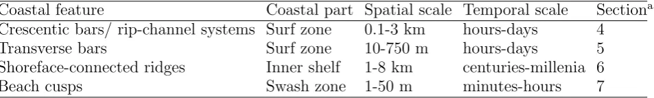
(raised areas of beach level) [Coco et al., 1999, and references therein]. These four features 65
are located in different parts of the coastal zone (i.e., at different water depths), and are 66
characterized by different spatial and temporal scales, as shown in Table 1 and Figure 2. 67
The relevance of these alongshore rhythmic patterns for coastal engineering is being 68
increasingly recognized for several reasons. Firstly, studying their dynamics allows identi-69
fication of important physical mechanisms that control coastal evolution. In particular, it 70
where there is still a significant lack of knowledge on such important process (e.g., swash 72
zone and inner surf zone) [Soulsby, 1997]. Secondly, these alongshore rhythmic morpho-73
dynamic patterns have a direct impact on the shoreline by creating areas of erosion and 74
deposition [Komar, 1998;MacMahan et al., 2006]. The presence of beach cusps and trans-75
verse bars implies an erosion of the shoreline in their embayments, and crescentic bars 76
and shoreface-connected ridges affect wave refraction and breaking, creating patterns in 77
the nearshore flow circulation that can cause erosional hot spots [Sonu, 1973;Wright and 78
Short, 1984;Benedet et al., 2007]. Furthermore, beach cusps are notable morphodynamic 79
features because they occur in the swash zone, a region whose dynamics are not yet well 80
understood but which forms the physical interface between the land and the sea, where 81
the effects of erosion/deposition are most clearly seen. In the surf zone, sandy bars are a 82
natural protection of the beach: waves dissipate part of their energy on the bars and the 83
bars can also provide sand to the beach as they can migrate onshore. Furthermore, the 84
alongshore migration of surf zone bars can cause (additional) erosion/deposition patterns 85
near coastal structures that are generally not considered in engineering projects. It is also 86
important to understand the horizontal circulation induced by surf zone bars since the as-87
sociated currents enhance transport and exchange of pollutant or floating matter [Castelle 88
and Coco, 2013]. Further, although surfers take advantage of rip currents occurring in 89
between sand bars to move offshore, such currents are dangerous for swimmers, being 90
one of the most lethal natural hazards worldwide [Dalrymple et al., 2011]. On the con-91
tinental shelf, shoreface-connected ridges are of interest to coastal engineering as sources 92
for extraction of sand (e.g., for beach nourishment or for the construction industry) and 93
de Meene and van Rijn, 2000]. Also, due to their alongshore migration, they can produce 95
the infilling of navigation channels and affect pipeline burial. Shoreface-connected ridges 96
also have an interest for biologists since they provide favorable conditions for benthic life 97
and fish [Slacum et al., 2010], in particular on their sheltered landward side (where grain 98
size is smaller). From a geologic point of view, all these morphodynamic features are of 99
interest because they lead to depositional rhythmic patterns that can be detected in the 100
stratigraphy, and thus provide insight into the long-term evolution of the coast. In par-101
ticular, shoreface-connected ridges, having evolved over thousands of years, can be traced 102
in and dated from cores [McBride and Moslow, 1991]. 103
Rhythmic morphodynamic patterns are the result of waves and currents that erode 104
and transport sediment by exerting shear stresses at the sandy sea bed. The conver-105
gence/divergence of sediment transport produces bed level changes, which feedback into 106
the wave and current fields. Rhythmic morphologic patterns grow very often due to feed-107
back mechanisms(the so-called self-organization theory), without a corresponding spatial 108
pattern in the hydrodynamic forcing (the latter being essential in the so-called template 109
theories) [Coco and Murray, 2007]. The key message of the present contribution is that, 110
despite the fact that beach cusps, surf zone bars and shoreface-connected ridges have dif-111
ferent scales and occur in different areas of the coastal zone, they nevertheless have one 112
important aspect in common: their formation, migration and long-term evolution can be 113
explained by the advection of the depth-averaged sediment concentration (DASC) by the 114
depth-averaged current. As each feature is associated with different types of water motion, 115
each has its own typical spatial distribution of sediment concentration. The aim of this 116
the development of these alongshore rhythmic coastal morphodynamic patterns. Previous 118
studies focusing on these distinct features will be reviewed and linked, thereby showing 119
that, by using a specific formulation of the equations, the convergence/divergence of sed-120
iment transport can be understood in a remarkably simple way, from the joint action 121
of the gradients in the DASC and the current perturbations produced by the evolving 122
morphologic pattern. This formulation is a powerful tool to get insight into the underly-123
ing feedback mechanisms that explain why features with a specific spatial pattern (e.g., 124
up-current orientation of shoreface-connected ridges and transverse bars, see Figure 2) 125
grow and migrate [e.g., Falqu´es et al., 2000; Calvete et al., 2001; Caballeria et al., 2002; 126
Ribas et al., 2003; Calvete et al., 2005; Dodd et al., 2008; Ribas et al., 2012]. The physical 127
mechanisms for the saturation of the growth of the features or for their decay can also 128
be explored with this technique [e.g., Garnier et al., 2006, 2008; Vis-Star et al., 2008; 129
Garnier et al., 2013]. 130
The first step is to present and discuss the formulation and methodology, based on the 131
DASC, which have been successfully used to understand and model the characteristics 132
of coastal patterns. In existing publications, different versions of this formulation were 133
presented, corresponding to the specific morphodynamic features being studied. Here we 134
will present the overall theory, the underlying hypotheses and the physical interpretation 135
of the equations. The model framework and most important physical laws and processes 136
governing the dynamics of the currents, the waves and the sediment at the coast are 137
presented in section 2. Since this contribution focuses on the morphologic evolution, 138
some technical details of the hydrodynamic processes will be given in appendices. The 139
and the methodology that allows understanding rhythmic pattern formation is described. 141
The second step is to review the key studies that apply this formulation to the development 142
of the four specific morphologic patterns mentioned above (Figure 2): crescentic bars 143
(section 4), transverse bars (section 5), shoreface-connected sand ridges (section 6) and 144
beach cusps (section 7). A physical and transparent explanation, based on the DASC, will 145
be provided of why alongshore rhythmic patterns of a certain shape grow and sometimes 146
migrate. Each of these four sections can be read independently of the others. Finally, 147
the most important conclusions are summarized in section 8 and a list of important open 148
issues for future research is included in section 9. 149
The four selected patterns have in common the presence of a coastline and an underlying 150
topography with a cross-shore slope (sloping beach, sloping shelf), which clearly distin-151
guishes an alongshore and a cross-shore coordinate. Also, they occur on wave-dominated 152
sandy coasts (without vegetation) that are uninterrupted in the alongshore direction at 153
the length scale of the studied feature. We do not cover other coastal morphodynamic 154
patterns such as ripples, megaripples, tidal sand waves, tidal sand banks, sorted bed-155
forms, cuspate shorelines and km-scale shoreline sand waves. A review on ripples, tidal 156
sand banks and tidal sand waves can be found inBlondeaux [2001]. Gallagher [2011], and 157
references therein, studied the formation of megaripples. A review on sorted bedforms 158
(or rippled scour depressions, related to a physical mechanism based on sediment sorting) 159
and large-scale cuspate shorelines was presented by Coco and Murray [2007]. Km-scale 160
shoreline sand waves have been studied by van den Berg et al. [2012] and references 161
2. COASTAL MORPHODYNAMICS, THE MODEL FRAMEWORK
Coastal morphodynamics is the research field that studies the mutual interactions be-163
tween the sea bed morphology and coastal hydrodynamics through sediment transport 164
[Wright and Thom, 1977]. These interactions are included in the process-based coastal 165
area models [Amoudry and Souza, 2011] (Figure 3). The sea bed level and the shoreline 166
of sandy coasts change due to the divergence/convergence of sediment transport, which 167
itself is driven by the bed shear stresses exerted by the flow velocities related to the cur-168
rents, the incoming waves and the turbulence. Changes in bed level in turn affect these 169
hydrodynamic processes, so feedback mechanisms occur. 170
It is important to keep in mind that those processes can occur at several time scales so 171
that the corresponding variables and equations are commonly time-averaged to just keep 172
the dynamics at the scale of interest. In particular, each morphological feature has its 173
own morphodynamic time scale, Tm, defined as that at which significant morphological 174
changes occur. This scale is roughly Tm = O(104s) for beach cusps, Tm = O(105s) for 175
surf zone bars and rip channels and Tm =O(1010s) for shoreface-connected sand ridges. 176
Figure 4 shows the frame of reference commonly used in coastal morphodynamic models. 177
The domain represents a sea that is bounded by an alongshore uniform coast. They-axis 178
is oriented in the alongshore direction, thex-axis is perpendicular to it, withxthe distance 179
to the coastline and thez-axis is vertical. 180
2.1. Coastal sediment transport and bed evolution
Conservation of sediment mass is the key equation of coastal morphodynamics and, 181
after some assumptions that are described in Appendix A, can be cast into 182
Here ∇⃗ = (∂/∂x, ∂/∂y) is the horizontal nabla operator, ⃗q(x, y, t) is the net transport 184
of sediment per unit width (total volume of sediment crossing the horizontal unit length 185
per unit time, m2s−1), h(x, y, t) = z
b(x, y, t)−zb0(x) is the bed elevation with respect 186
to an alongshore uniform background bathymetry, z =zb0(x), and p is sediment porosity 187
(typically p ∼ 0.4). The adjective net means that ⃗q(x, y, t) results from a time-average 188
on a time interval that is short enough with respect to the morphological time scale we 189
are interested in. Equation (1) states that the bed level rises (∂h/∂t >0) at the locations 190
where sediment transport converges (∇ ·⃗ ⃗q < 0) and vice versa (Figure 7). 191
To evaluate bed level changes sediment transport must therefore be computed. Sediment 192
transport in the coastal environment is a complex process that depends on the mechanics 193
of sediment grains subject to forces exerted by waves and currents. It takes place both 194
in suspension (suspended load) and in contact with the bed (bed load, which may include 195
sheet flow) [Soulsby, 1997]. Sediment transport is still poorly understood and hard to 196
predict accurately [Amoudry and Souza, 2011], due to the complexity of the processes 197
involved. On the other hand, field observations suggest that the dynamics of beach cusps, 198
rhythmic surf zone bars and shoreface-connected ridges is associated to the action of 199
intense currents involving net water mass flux. These observations motivate the working 200
hypothesis that the net sediment transport,⃗q, depends on the depth-averaged current, ⃗v, 201
(net water volume flux per unit width divided by net water depth, see section 2.2) through 202
the formula 203
⃗
q=α⃗v , (2)
204
in which case the expression is exact and α is the depth-integrated volumetric sediment 207
concentration (m3/m2). As is further explained in Appendix A, additional sediment 208
transport occurs in the cross-shore direction due to a number of sources including gravity 209
combined with bottom slope, wave nonlinearities and undertow. Here it is assumed that 210
the joint action of the various cross-shore sediment transport sources, not described by 211
equation (2), determines an equilibrium cross-shore beach and inner shelf profile. This 212
profile is chosen as the background bathymetry, zb0(x), and in the absence of current, ⃗v, 213
it is assumed to be stable. The possible unbalance in cross-shore sediment transport due 214
to any deviation, h(x, y, t), just tends to drive the bathymetry back to equilibrium. This 215
is represented by a slope term that is added to equation (2), which becomes 216
⃗q=α⃗v−γ ⃗∇h . (3)
217
The rationale behind equation (3) is that oscillatory motions mobilize (or stir) the sed-218
iment, due to either the orbital velocities at the bed or the turbulent vortices created 219
by breaking waves, without producing a transport. The current increases the stirring 220
and transports the sediment (as illustrated in Figure 6). The stirring is represented by 221
the sediment load α and the slope coefficient γ, which can depend (nonlinearly) on local 222
quantities such as the current magnitude |⃗v|, the amplitudes of the wave orbital velocity 223
and the turbulence-induced velocity, the sediment properties and the water depth D. If 224
the velocities at the bed are smaller than a critical value, α and γ are zero. This formu-225
lation works reasonably well, in the sense that it captures the overall characteristics of 226
the processes [Fredsoe and Deigaard, 1992;Soulsby, 1997; Camenen and Larroud´e, 2003]. 227
bathymetry to the alongshore uniform equilibrium and that the sediment transport is in 230
equilibrium with the local hydrodynamics so that possible lags are neglected. 231
The sediment load α in the first term of equation (3) is the total volume of sediment 232
in motion per horizontal area unit (m3/m2), and can also be interpreted as a ‘stirring 233
function’ [e.g., Falqu´es et al., 2000] if this term is understood as describing sediment 234
being stirred (by waves and currents) up to load α and then being transported by the 235
current. Characteristic values of α range from 10−5 m3/m2, for bedload conditions, to 236
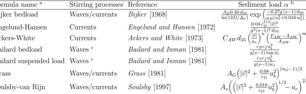
10−3 m3/m2, for total load conditions [Soulsby, 1997]. Table 2 shows examples of the 237
α function for six standard sediment transport formulas that can be cast in the form 238
of equation (3), all of them described in detail in Soulsby [1997]. An illustration of the 239
applicability of many of these different sediment transport parameterizations (and others) 240
is given in Camenen and Larroud´e [2003]. As described in Soulsby [1997], the existing 241
formulas have been extensively calibrated, although mostly in wave flumes or outside 242
the surf zone. Under breaking waves, the strong turbulent vortices can have a significant 243
amplitude at the bed and add to the sediment stirring by the current and the wave orbital 244
velocity [Voulgaris and Collins, 2000; Butt et al., 2004]. This process is not included in 245
any of the standard sediment transport formulas (Table 2) but can be included with an 246
adequate expression of the α function. For example, Reniers et al. [2004] added this 247
process in the α of the Soulsby and van Rijn formula and Ribas et al. [2011] modified it 248
and showed its importance for the dynamics of rhythmic surf zone bars. In the surf zone 249
applications the stirring by turbulent vortices as implemented by Ribas et al. [2011] will 250
be included. 251
As explained in the previous section, to calculate the sediment transport some hydro-252
dynamic variables, such as the current, the water depth and the wave orbital velocity, 253
must be computed. Water motion in the coastal zone occurs at different time scales. On 254
the coasts studied here, incoming waves are the most obvious motion to the eye. The 255
characteristic time scale of waves is provided by their period, Tw, which typically ranges 256
between 1 and 20 s. At shorter time scales turbulent motions take place. Since the rela-257
tive amount of sediment carried by the water motion is small (volumetric concentration 258
of sediment hardly reaches O(10−2)) the bed level typically changes at a characteristic 259
time scale (morphodynamic time scale), Tm ≫ Tw. Therefore, it is sufficient to consider 260
time-averaged hydrodynamic variables and thus filter out the fast dynamics at the time 261
scales of waves and turbulence. This means that the hydrodynamics is decomposed into 262
two components: a) mean motions and b) ”fast” fluctuating motions. Of course, waves 263
and turbulence affect the dynamics of the system but their effects are considered only 264
through averages that are described by the corresponding hydrodynamic forces on the 265
mean motions. Therefore, all hydrodynamic variables are time-averaged on a time scale 266
Tw. An exception will be made when describing the dynamics of the swash zone, where 267
the time average needs to be made on a shorter time scale, filtering only the turbulent 268
motions but not the waves. 269
Another important assumption is that we focus on morphodynamic features located in 270
shallow waters and the horizontal scales involved in these features are at least one order 271
of magnitude larger than the vertical scales. It is therefore reasonable to expect that their 272
dynamics can be understood within the framework of the depth-integrated shallow water 273
variables describing the mean hydrodynamic motions (i.e., the dynamics of the water 275
columns) are the depth-averaged current, i.e., the time-averaged water volume flux per 276
unit width divided by the time-averaged water depth,⃗v(x, y, t) (hereinafter simply referred 277
to as current), and the time-averaged free surface level,zs(x, y, t). 278
Conservation of water mass is one of the fundamental laws for the mean hydrodynamic 279
motions. Its depth-integrated formulation reads 280
∂D ∂t +
⃗
∇ ·(D⃗v) = 0 , (4)
281
where D=zs−zb is the time-averaged water depth. The quantity D⃗v is the volumetric 282
flux of water per unit width entering a water column [Svendsen, 2006]. Equation (4) states 283
that if there is convergence of water flux (i.e.,∇·⃗ (D⃗v)<0, meaning that a net quantity of 284
water flows into the water column) an increase in water depth will occur (i.e.,∂D/∂t > 0, 285
for instance by increasing the free surface levelzs, see Figure 5a). Note that, in the swash 286
zone, an extra term may appear on the right hand side (RHS) of equation (4), related to 287
the infiltration of water into the bed [Dodd et al., 2008]. 288
The momentum balance for time and depth-averaged currents 289
∂⃗v
∂t +⃗v ·∇⃗⃗v =−g ⃗∇zs+ ⃗τb
ρD +
⃗τw
ρD +
1
ρD∇ ·⃗ (R−S) , (5)
290
is the other fundamental law governing the mean motions. The LHS (left hand side) is 291
the horizontal acceleration of the water columns and the RHS consists of the forces per 292
mass unit acting on them. The first term on the RHS represents the pressure gradient 293
force per unit mass due to gradients of the free surface level. The second term involves 294
the net bed shear stress,⃗τb,which produces frictional forces on the flow and also the wind 295
Reynolds stress tensor, R, and the wave radiation stress tensor, S, are 2D second order 297
symmetric tensors that describe the net depth-integrated transfer of momentum that are 298
due to turbulence and waves, respectively. Their divergence, whose x- and y-components 299
are (e.g., ∇ ·⃗ S) 300
∂Sxx
∂x +
∂Sxy
∂y ,
∂Syx
∂x +
∂Syy
∂y , (6)
301
results in a force acting on the water columns. For beach cusps Sis absent since the time 302
average is made on a time scale shorter than Tw, filtering the turbulent motions but not 303
the waves. Moreover, for large scale features O(1-10 km), appearing on the continental 304
shelf, the Coriolis volumetric force is added on the RHS of equation (5). 305
Knowing the bed level zb(x, y, t), the system of the hydrodynamic equations (4) and (5) 306
is not closed mainly because the stress tensors depend on the fast fluctuating hydrody-307
namic components, i.e., turbulence and waves. Turbulent stresses play a secondary role 308
and are modeled with the standard eddy viscosity approach [Svendsen, 2006] so that they 309
are proportional to ∇⃗v components through a mixing coefficient that depends on wave 310
energy dissipation. However, wave radiation stresses are crucial in the surf zone as they 311
provide the main driving force for the currents. They depend on wave energy density, on 312
the propagation direction and on the ratiocg/c(cg, c being the group and phase celerities) 313
[Longuet-Higgins and Stewart, 1964; Svendsen, 2006]. Essentially, when waves approach 314
the coast and feel the sea bottom they start refracting, shoaling and breaking, varying 315
their energy density and direction. These changes cause in turn gradients in the radiation 316
stresses producing net forces on the water column. The net bed shear stresses in equa-317
small bedforms. This is not straightforward and different options can be used [e.g., Fed-320
dersen et al., 2000]. The specific equations and parameterizations used to describe the 321
different features can be found in Caballeria et al. [2002] (surf zone bars), Calvete et al. 322
[2001] (shoreface-connected ridges), and Dodd et al.[2008] (beach cusps). 323
Although the individual wave motions are not resolved in the present formulation, the 324
knowledge of the time-averaged properties of waves is nevertheless crucial. These include 325
wave energy density, energy dissipation, orbital velocity amplitude, angle and wavenum-326
ber. In fact, all these quantities can be computed in terms of the root-mean-square height, 327
H(x, y, t), the wavenumber, k(x, y, t), and the wave angle, θ(x, y, t) (Figure 4) and these 328
three variables can be evaluated using the dispersion relation, the wavenumber irrotation-329
ality and the wave energy balance. The details and the corresponding set of equations, 330
which are subsequently coupled to equations (4) and (5), are described in Appendix B. 331
A common assumption regarding coastal morphodynamics is the so-called quasi-steady 332
approximation. It consist of dropping out all the time derivatives from the hydrodynamic 333
equations (4) and (5) but not from the bed evolution equation (1). It is not an essential 334
step for the methodology explained in this contribution but it facilitates the physical 335
interpretation of the equations. For instance, the mass conservation equation (4) becomes 336
⃗
∇·(D⃗v) = 0, which means that there is no net water transport into or out from the water 337
column. A gradient inD then implies a change in⃗v (Figure 5b shows a 1D example of a 338
current increase due to a decreasing water depth). 339
The quasi-steady assumption means that the hydrodynamics is in equilibrium with the 340
morphology all the time, i.e., the hydrodynamic variables are assumed to adapt instan-341
assumption suppresses any oscillatory solution of equations (4) and (5) like infragravity 343
waves,shear waves,low frequency eddies and tidal waves. The first three types of motion 344
occur with periods ranging from about 20 s to O(103 s) [Reniers et al., 2004] while tides 345
occur at periods of O(104 s). The quasi-steady approximation can be applied if the os-346
cillatory water motions do not affect significantly the morphologic evolution. This is not 347
the case for beach cusps, which are in fact closely linked to the unsteady wave motion as 348
it is expressed in the uprush and backwash of the waves. On the other hand, despite low 349
frequency eddies may affect crescentic bar dynamics [Reniers et al., 2004] and infragravity 350
waves (edge waves) had earlier been thought to be the primary cause of rhythmic surf zone 351
features (Holman and Bowen [1982] and others, see sections 4.2 and 5.2), it is nowadays 352
accepted that these low-frequency oscillatory motions are not essential for the formation 353
of rhythmic bars in the surf zone [Blondeaux, 2001; Coco and Murray, 2007]. Similarly, 354
although tidal oscillations mildly affect the evolution of shoreface-connected sand ridges, 355
they are not essential for explaining their formation [Walgreen et al., 2002]. The quasi-356
steady assumption is therefore applied to understand the dynamics of surf zone rhythmic 357
bars and shoreface-connected sand ridges. 358
3. FORMULATION AND METHODOLOGY BASED ON THE
DEPTH-AVERAGED SEDIMENT CONCENTRATION
3.1. Bed evolution equation
A formulation of the bed evolution equation based on the depth-averaged sediment 359
concentrationis now derived. For this, we substitute⃗qfrom equation (3) into equation (1) 360
to obtain the so-called bed evolution equation (BEE), 361
where C = α/D is the total sediment load divided by the water depth. In the present 363
contribution, C is interpreted as a depth-averaged sediment concentration (DASC) and 364
it includes both bedload and suspended load. Some authors [Falqu´es et al., 2000] have 365
called it ‘potential stirring’ but here we use the name DASC because it is related to a 366
variable that can be measured. In the outer surf zone and the continental shelf, bottom 367
changes occur at depths larger than O(1 m). In the inner surf zone and the swash zone, 368
water depths range between 0.1−1 m. Given that α ≤ 10−3 m3/m2 (see section 2.1), 369
characteristic values of C range from 10−7 to 10−2 m3/m3 (C could be higher only in 370
the very shallow swash zone). The left hand side (LHS) of equation (7) quantifies the 371
bottom changes. The first term on the RHS describes the erosion/deposition produced 372
due to the advection of C by the depth-averaged current⃗v when there are gradients of C 373
(section 3.2 is devoted to explain in depth the physical interpretation of this term). The 374
second term on the RHS describes the deposition (erosion) that occurs when water flux 375
converges (diverges). The third term on the RHS is a slope-induced diffusive term and 376
tends to damp the gradients in bed level. 377
If the quasi-steady hypothesis can be assumed (i.e., for surf zone and inner shelf fea-378
tures), the mass conservation equation (4) becomes ∇ ·⃗ (D⃗v) = 0 (see section 2.2) and the 379
BEE becomes 380
(1−p)∂h
∂t =−D⃗v· ⃗
∇C +∇ ·⃗ (γ ⃗∇h) . (8)
381
In the application at the swash zone (beach cusp development), where the quasi-steady 382
hypothesis does not hold, equation (7) is used, with an additional term related to water 383
3.2. Erosion/deposition processes
Equation (8) gives the time evolution of the bed level deviations at any location as a 386
function of the water depth, D, the depth-averaged current, ⃗v, and the gradient of the 387
DASC,C. It is not a closed equation since it needs the knowledge of⃗vand the distribution 388
ofC. The powerful advantage of equation (8), with respect to the original equation (1), is 389
that it allows for an interpretation of the erosion/deposition processes, in terms of⃗v and 390
⃗
∇C, which might be known from field observations, from numerical simulations or just 391
qualitatively from physical reasoning. 392
According to equation (8),⃗v·∇C⃗ >0 will tend to induce bed erosion (∂h/∂t <0) and 393
⃗v·∇C⃗ < 0 will tend to induce bed accretion (∂h/∂t > 0). In words, any current with a
394
component in the direction of the gradient inC will produce erosion and any current with
395
a component that opposes this gradient will cause accretion(Figure 8). This behavior can 396
be physically understood from the fact that C is in local equilibrium with the flow, i.e., it 397
is the depth-averaged sediment concentration of the water column corresponding to the 398
stirring by the local hydrodynamics (section 2.1 and Appendix A). If C increases along 399
the flow (⃗v·∇C⃗ >0), water with little amount of C will move to places where the stirring 400
by the hydrodynamics allows for larger C. Therefore, more sediment will be picked up 401
from the bed underneath the water column, which will hence be eroded (Figure 8a). The 402
contrary will happen ifC decreases along the flow (Figure 8b). 403
3.3. Linearized bed evolution equation
In order to understand the dominant mechanisms involved in the initial formation of 404
the features of interest, it is convenient to assume that the state of the system is a 405
defined in section 2.1) and a perturbed state, with small amplitude perturbations that 407
evolve from the equilibrium state [Dodd et al., 2003]. The equilibrium state represents the 408
mean dynamic balance in the absence of rhythmic features. It consists of an alongshore 409
uniform equilibrium profile zb0(x) (already mentioned in section 2.1), a depth-averaged 410
sediment concentration C0(x), a water depth D0(x) that includes the wind- or wave-411
induced set-up/set-down, and often an alongshore current V0(x). The set-up (set-down) 412
is an over-elevation (under-elevation) of the free surface level in the coastal zone forced by 413
the cross-shore transfer of momentum after waves break or by wind-induced cross-shore 414
forces. The alongshore current is forced by the alongshore momentum transfer produced 415
after oblique waves break, by wind-induced alongshore forces or by free surface gradients. 416
A schematic representation of the alongshore current and the wave-induced set-up can be 417
seen in Figure 4. 418
Small perturbations in bed level,h(x, y, t) (the bed level deviations defined in section 2.1, 419
but now assumed to be small), concentration, c(x, y, t), depth, d(x, y, t), and current, 420
(u(x, y, t),v(x, y, t)), are added to the equilibrium. The total variables then read 421
zb =zb0+h , C =C0 +c , D=D0+d and ⃗v = (0, V0) + (u, v) . (9) 422
Substituting these expressions into equation (8) and only retaining the terms that are 423
linear in the small quantities (u, v, c, d and h), yields the linearized BEE, 424
(1−p)∂h
∂t =−D0u dC0
dx −D0V0 ∂c ∂y + ∂ ∂x ( γ0 ∂h ∂x ) + ∂ ∂y ( γ0 ∂h ∂y ) . (10) 425
Hereγ0 is the equilibrium value of theγ coefficient in equation (8). 426
Equation (10) shows that the small bed level changes of a known equilibrium state can 427
ponent of the current, u, and the alongshore gradients of the perturbation of the DASC, 429
∂c/∂y. The first RHS term of equation (10) leads to deposition (erosion) if u dC0/dx is 430
negative (positive). The second RHS term of equation (10) leads to deposition (erosion) if 431
V0∂c/∂y is negative (positive). Note that ifV0 = 0, the second RHS term disappears and 432
erosion/deposition processes only depend onuand the cross-shore gradient of the equilib-433
rium DASC, dC0/dx. The last two RHS terms of equation (10) have a diffusive effect on 434
the bed perturbations. The first derivation of a linearized BEE similar to equation (10) 435
for the nearshore was made by Falqu´es et al. [1996]. 436
3.4. Erosion/deposition patterns: global analysis
The equations and analysis of the previous sections, based purely on equations (8) or 437
(10), are local in the sense that these equations describe the bed level evolution in one 438
location due to local convergence/divergence of the sediment transport. Since this con-439
tribution aims at understanding the development of morphologic patterns that grow and 440
migrate on the whole domain, it is essential to understand the erosion/deposition patterns 441
occurring on the whole domain. As an example, given a morphological feature consist-442
ing of alongshore alternating bars and troughs, Figure 9 shows what erosion/deposition 443
patterns would produce (a) pure growth, (b) growth and down-drift migration, (c) pure 444
down-drift migration, (d) decay and down-drift migration, and (e) pure decay of the fea-445
ture. Thereby, it is essential to analyze the effect integrated on the whole domain of the 446
different terms in equations (8) or (10) in order to evaluate their influence on growth, 447
decay or migration of the features. As a first step, this can be done in a qualitative way, 448
i.e., by visual observation of the erosion/deposition patterns created by each of the terms 449
term on the RHS of equation (8), and consistently with the local analysis presented in 451
section 3.2, if the regions withh >0 and the current opposing the gradients in DASC (or 452
h < 0 and the current running with the gradients in DASC) dominate over the regions 453
where the contrary occurs, this term will contribute to the growth of the feature. Al-454
ternatively, a quantitative global analysis of the equations can be performed by taking a 455
specific average over the horizontal domain of the different terms in equations (8) or (10). 456
The global effect of each term on the development of the morphological patterns can then 457
be studied quantitatively. The technical details of how such a quantitative global analysis 458
is performed are given in Appendix C. 459
In the next sections it will be demonstrated that, for a wide range of alongshore rhythmic 460
morphological patterns, the global effect of the first RHS term of equation (10) essentially 461
contributes to the initial growth of the features, the second RHS term essentially con-462
tributes to their alongshore migration (in the presence of an alongshore current), and 463
the last two terms produce decay of the features. This is a powerful result: the ’sponta-464
neous’ breaking of alongshore uniformity of the nearshore bathymetry and the emergence 465
of alongshore rhythmic morphological patterns can be understood by knowing only the 466
cross-shore gradient of the equilibrium DASC, dC0/dx and the cross-shore perturbation 467
of the induced horizontal currents, u (first RHS term of equation (10)). 468
3.5. Methodology to use the DASC to explain pattern development
The development of four different alongshore rhythmic morphodynamic patterns are 469
explained in the next sections: two surf zone patterns (crescentic bars and transverse 470
(beach cusps). The following three steps are taken to use the DASC to understand the 472
formation of these morphological patterns. 473
First, it is essential to have information on the gradients in DASC. This quantity is 474
difficult to measure in the surf zone due to the highly complex dynamics of sediment 475
transport under breaking waves [Soulsby, 1997] and it is also highly unknown in the 476
swash zone. Thereby, very often the formulations are inferred from laboratory data and 477
theoretical reasoning. Different parameterizations found in the literature (like those in 478
Table 2) lead to different results forC, which can strongly affect the morphological changes. 479
Here, physical reasons will be presented as to what C profiles are expected in the areas 480
where features develop. Also, one of the formulas in Table 2 (which has been extensively 481
calibrated against data) will be applied to substantiate the reasoning. Since the bed 482
evolution depends on the gradients of the concentration (section 3.2), it is crucial that the 483
parameterizations of sediment transport adequately represent not only the magnitude of 484
DASC, but especially the gradients of DASC. 485
Second, some information on the hydrodynamics induced by the growing feature is 486
needed. This information can be obtained by measurements and/or with the hydrody-487
namic module of the morphodynamic models. The latter is usually quite robust, i.e., there 488
is little difference between the different models, even though different parameterizations 489
are used for the bed shear stresses, the turbulence-induced effects, wave energy dissipa-490
tion through breaking, etc. Here, the focus will be on describing the horizontal currents 491
(and especially the cross-shore component u) associated with each feature, discussing in 492
Third, a global analysis (either qualitative or quantitative) of the linearized BEE (10) 494
must be performed in order to understand the erosion/deposition patterns, created by the 495
joint action of the horizontal currents and the gradients in DASC, that causes the initial 496
formation of the features. This allows understanding the initial shape of the pattern, 497
its initial growth and migration rates, and under which climate conditions the feature 498
develops. 499
Finally, a global analysis (either qualitative or quantitative) of the nonlinear BEE (8) is 500
performed to understand the finite amplitude behavior of the features: saturation of the 501
growth and changes in shape and migration rate. In some cases, this analysis also allows 502
explaining the destruction of the features by certain climate conditions. 503
4. CRESCENTIC BARS
4.1. Characteristics of observed crescentic bars (and rip channels)
Crescentic bars are located in the surf zone of micro to meso-tidal sandy beaches [Lipp-504
mann and Holman, 1990; van Enckevort et al., 2004; Lafon et al., 2004] (Figures 1a 505
and 2g). The alongshore spacing between crescentic bar horns is relatively constant for a 506
specific system. They have been reported at different scales with a mean spacing ranging 507
from tens of m up to 2-3 km. Crescentic bars are sometimes also called rip channel sys-508
tems because the rip channels are a striking and well known characteristic of them [van 509
Enckevort and Ruessink, 2003]. Note, however, that rip channels, i.e., bed depressions or 510
cross-shore oriented channels in the surf zone where rip currents concentrate, can also be 511
observed without the presence of crescentic bars (see, e.g., MacMahan et al. [2005] and 512
Crescentic bars are linked to shore-parallel bars, which are alongshore uniform sand 514
bars parallel to the coast. The latter form in medium sand beaches during high-energy 515
wave events. Crescentic bars develop out of the shore-parallel bar during decreasing wave 516
energy (Figure 10), i.e., during post-storm conditions. In the widely accepted beach 517
state classification [Wright and Short, 1984; Lippmann and Holman, 1990], such process 518
is classified as the down state transition from the Longshore Bar and Trough state to 519
the Rhythmic Bar and Beach (RBB) state. Crescentic bars can become shore-parallel 520
again in the reverse (up state) transition if wave energy increases again (Figure 10). 521
The latter process is called bar straightening or morphologic reset. Recent studies have 522
stressed the effect of wave obliquity in the transitions between shore-parallel and crescentic 523
bars, revisiting the traditional classification ofWright and Short [1984]. They found that 524
crescentic bars seem to develop preferably for normal wave incidence and bar straightening 525
occurs for highly oblique waves [Holman et al., 2006;Thornton et al., 2007;Splinter et al., 526
2011; Price and Ruessink, 2011]. 527
Along beaches with crescentic bars the shoreline often features undulations with a sim-528
ilar alongshore spacing. Since this spacing is typically significantly larger than the one 529
of ordinary beach cusps, these undulations are called megacusps [Thornton et al., 2007]. 530
The horns of the crescentic bars can connect to the shoreline and to the megacusp system 531
during long-lasting conditions of low wave energy (down state transition from the RBB 532
state to the Transverse Bar and Rip (TBR) state [Wright and Short, 1984; Ranasinghe 533
et al., 2004]). The resulting transverse bar system is a particular case of the four different 534
types of transverse bar systems that will be discussed in section 5. 535
The origin of crescentic bars was first explained with the so-called hydrodynamic tem-536
plate theory, in which the morphologic pattern is the result of a pre-existing similar pattern 537
in the hydrodynamics [see the review by Coco and Murray, 2007]. More specifically, their 538
formation was attributed to the pattern of near-bed velocities associated withedge waves 539
[Bowen and Inman, 1971; Holman and Bowen, 1982], which are alongshore propagating 540
trapped waves. Edge waves with alongshore spacings at the crescentic bar scale can be 541
generated by infragravity oscillations associated with the incident wind or swell waves. 542
However, more recent studies have shown that the edge wave hypothesis is only partially 543
consistent with available field data [Coco and Murray, 2007]. 544
The second theory, which was first suggested by Hino [1974], is that crescentic bars 545
emerge as a morphodynamic instability of the system with a shore-parallel bar. That 546
is, they emerge from a positive feedback between wave-driven currents and morphology, 547
starting from any perturbation of the featureless state. The first study modeling the 548
formation of a crescentic bar from a shore-parallel bar by self-organization was that of 549
Deigaard et al. [1999]. Falqu´es et al. [2000] described in more detail the physical mecha-550
nisms involved, emphasizing the role of the depth-averaged sediment concentration (called 551
potential stirring in that paper). The instability mechanism was called ‘bed-surf instabil-552
ity’ (term introduced by Falqu´es et al. [1996]) because it is essentially due to the positive 553
feedback between the sea bed perturbations and the distribution of wave breaking. Later 554
on,Calvete et al.[2005] used a more realistic model that reproduced many of the observed 555
characteristics of crescentic bars and confirmed the important role of the DASC in cres-556
centic bar formation. The self-organized origin of crescentic bars has been supported by 557
inghe et al., 2004; Reniers et al., 2004; Klein and Schuttelaars, 2006; Garnier et al., 2008; 559
Smit et al., 2008] making this theory currently more widely accepted than the hydrody-560
namic template theory. In the next section, the role of the DASC in the transformation 561
of shore-parallel bars into crescentic bars will be discussed based on the studies ofFalqu´es 562
et al. [2000],Calvete et al. [2005] and Garnier et al.[2008]. 563
4.3. Role of DASC in the formation mechanism
For the sake of simplicity, and since crescentic bars mainly develop for relatively small 564
wave incidence angles, the focus of this section is on the case of normally incident waves 565
(i.e., no alongshore current, V0 = 0). The case of oblique waves will be discussed later in 566
section 4.4. As explained in section 3, the joint effect of the gradients in DASC and the 567
horizontal circulation induced by the growing feature creates the erosion/deposition pat-568
terns that explain why the feature grows. The three steps of the methodology (section 3.5) 569
to explain crescentic bar formation when V0 = 0 are: 1) describing the cross-shore dis-570
tribution of the DASC (i.e., dC0/dx), 2) understanding the horizontal circulation induced 571
by the growing feature (i.e., u), and 3) analyzing the erosion/deposition patterns with 572
the linearized BEE (10) and the knowledge of dC0/dx and u. These steps are done in the 573
three following subsections. 574
4.3.1. Depth-averaged sediment concentration profile
575
As stated before, measuring the sediment concentration in the surf zone is difficult, 576
hence available data are scarce. However, the theory presented here is based on a simple 577
and robust property of the sediment concentration in the surf zone of barred beaches. 578
For moderate wave conditions, waves break predominantly over the shore-parallel bar 579
most of the sediment transport formula applied for the surf zone. More precisely, in surf 581
zones that are characterized by a shore-parallel bar waves can break on the bar (somewhat 582
seaward of it) if they have a sufficient height (Figure 11). This causes an intense sediment 583
resuspension in that area (by wave orbital velocities and turbulent vortices, if included), 584
i.e., the sediment loadα(equation 3) is maximum at a certain point on the seaward flank 585
of the bar. Furthermore, the water depth has a local minimum at the top of the bar and 586
increases onshore and offshore of the crest. Therefore, the depth-averaged concentration 587
(DASC, C = α/D) is maximum at a location x = xm slightly seaward from the crest. 588
Thus, there is an offshore-directed gradient in C for x < xm and an onshore-directed 589
gradient for x > xm. This qualitative behavior is reproduced by all the formulations for 590
nearshore sediment transport included in Table 2. As an example, the middle panel of 591
Figure 11 shows the DASC profile obtained with the Soulsby-van Rijn formula [Soulsby, 592
1997], extended to include an extra sediment stirring produced by turbulent vortices 593
[Reniers et al., 2004; Ribas et al., 2011]. 594
4.3.2. Rip current circulation
595
The horizontal circulation that is produced over an incipient crescentic bar (i.e., a shore-596
parallel bar with small-amplitude channels) is the well known rip current circulation. 597
For normally or nearly normal wave incidence, breaking waves over the small-amplitude 598
crescentic bar induce a circulation cell with offshore flow at the channels and onshore flow 599
at the shoals (Figure 12a). This is a robust characteristic that has been observed in the 600
field [MacMahan et al., 2006;Moulton et al., 2013] and in wave-basin experiments [Haller 601
et al., 2002; Castelle et al., 2010a], and that is also commonly reproduced by models 602
u (equation 10) can be assumed to have its maximum seaward-directed value (u > 0) in 604
the channels (i.e., where h <0) and its maximum shoreward-directed value (u <0) over 605
the shoals (i.e., where h > 0). The basic physics underlying this circulation is explained 606
in Appendix D. 607
4.3.3. Formation mechanism
608
Now, the joint morphodynamic effect of the gradients in DASC (C) and the horizontal 609
circulation can be inferred from the linearized BEE (10). Since we focus on the case of 610
normally incident waves, there is no alongshore current in the equilibrium state (V0 = 0) 611
and the second RHS term of equation (10) drops out. The gradient in C is offshore-612
directed over the bar crest, where the current flows onshore (negative u, see Figure 12a). 613
Thereby, u dC0/dx < 0 in equation (10), which means that the current carries sediment 614
from offshore, where C is largest, to the shoal (see section 3.2 and Figure 8). In the 615
channels, it is the other way around: the current flows offshore and it carries sediment from 616
the channel to offshore. In this way, the circulation will further erode the channels and 617
deposit the sand on the shoals. Thus a positive feedback will occur that will enhance both 618
the circulation and the bed undulation and the initially shore-parallel bar will develop rip 619
channels flanked by shoals (Figure 12b). In addition to that, and given that the position 620
of the maximum in DASC, x=xm, is close to the crest, the rip currents extend offshore 621
of this location and cause deposition of sediment seaward of it because the gradient in C 622
has an opposite sign there. Similarly, the onshore flowing part of the circulation will cause 623
erosion seaward of the shoals. Thus, the combination of the DASC and the circulation 624
creates not only channels and shoals on the bar but a mirrored pattern offshore of the 625
of alternating shoals and channels produces an undulation of the bar in plan-view, with 627
onshore protruding sections coinciding with the shoals over the bar and offshore protruding 628
sections at the rip channels. This is the typical crescentic bar morphology (Figure 10). 629
4.4. Finite amplitude behavior
The self-organization models cited in section 4.2 are able to reproduce the initial for-630
mation of the crescentic bars with the appropriate shape, but they are unable to explain 631
the saturation of growth of crescentic bars. The latter process was first simulated by 632
Garnier et al. [2008] (Figure 13). The specific mechanisms for the growth saturation 633
were explained by Garnier et al. [2010] with the use of the global analysis (methodology 634
described in Appendix C). The saturation of bar height, preventing the accreting shoals 635
to reach the sea surface, occurs mainly due to a weakening of the positive feedback (term 636
−D⃗v· ∇C in equation (8)) rather than to an increase of the damping caused by the dif-637
fusive transport. The positive feedback weakens but does not vanish: it balances with 638
the diffusive term (which remains constant), and therefore the latter is also essential to 639
the saturation process. The weakening of the positive feedback is related to changes in 640
bar shape rather than to the growth in amplitude. It turns out that the most important 641
change in shape is that the shoals widen and the channels narrow. More details of the 642
global analysis applied to the full saturation of crescentic bars are given in Appendix E. 643
Furthermore, the shoals shift shoreward and the channels seaward with the result that the 644
bars move overall onshore. This last result shows that the current circulation associated 645
with well developed crescentic bars system contributes to the attachment of the crescentic 646
Another important finite amplitude behavior of the crescentic bar systems is the bar 648
straightening. Using the global analysis,Garnier et al.[2013] explained why a developed 649
crescentic bar straightens due to wave obliquity. Oblique waves inhibit the formation of 650
rip channels and straighten crescentic bars because they weaken the rip current intensity 651
and cause a down-wave shift of the rips with respect to the channels (i.e., a phase lag 652
between the rips and the channels). This weakens the positive feedback between flow and 653
morphology given by the term −D⃗v· ∇C in equation (8). A more detailed explanation is 654
included in Appendix E. 655
4.5. Discussion
All the analysis presented so far in this section concerns a single crescentic bar system. In 656
nature, two crescentic bars can coexist in the same beach at different cross-shore positions 657
[van Enckevort et al., 2004; Castelle et al., 2007; Price and Ruessink, 2011]. In general, 658
such double bars do not behave independently. The outer crescentic bar may emerge from 659
self-organization (independently of the inner bar), it then induces alongshore variability 660
in the onshore hydrodynamics, which in turn forces the morphologic response of the inner 661
bar. This behavior is called morphologic coupling [Castelle et al., 2010b]. It is important 662
to notice that even in the case of morphologic coupling, the self-organization feedbacks 663
between flow and morphology described in section 4.3 still affect the evolution of both 664
bars [Coco and Calvete, 2009; Thiebot et al., 2012]. Particularly, for a double crescentic 665
bar system the DASC profile exhibits a local maximum over each bar system. 666
Although the present contribution is dedicated to rhythmic patterns observed in open 667
beaches, it should be stated that crescentic bars are also observed in embayed beaches 668
coastal structures. The presence and characteristics of those bars are then conditioned by 670
the length of the beach (i.e., distance between headlands) but they still seem to emerge 671
from the basic positive feedback described in section 4.3 [Castelle and Coco, 2012]. 672
The results presented in this section are taken from previous studies that consider 673
idealized simplified conditions. Particularly these studies consider an initial bathymetry 674
that is alongshore uniform [Falqu´es et al., 2000;Garnier et al., 2008, 2010] or a bathymetry 675
with a very specific variability [Garnier et al., 2013]. Furthermore, the incoming wave 676
field is assumed to be time invariant and alongshore uniform. Other modeling studies have 677
discussed the variability in the wave forcing [Reniers et al., 2004;Castelle and Ruessink, 678
2011] or in the initial bathymetry [Tiessen et al., 2011;Smit et al., 2012]. They show that 679
this affects the characteristics (e.g., spacing between rip channels) and the dynamics (e.g., 680
growth times) of the crescentic bars. However, the feedbacks between flow and morphology 681
associated with the advection of DASC by the rip currents described in section 4.3 still 682
play a key role. 683
5. TRANSVERSE BARS
5.1. Characteristics of observed transverse bars
Apart from the crescentic bars discussed in section 4, the surf zone can also display an-684
other kind of morphodynamic feature consisting of several transverse bars separated by an 685
approximately constant alongshore distance (Figures 1b,c and 2f). The alongshore spac-686
ing is defined as the distance between successive bar crests. They are typically attached to 687
the shoreline and extend into the seaward direction, either approximately perpendicular 688
to the coastline or with a certain oblique orientation if an alongshore current is present. If 689
down-current (up-current) oriented bars (Figure 14). However, we use the general term 691
transverse bars to refer to all of them, a term introduced by Shepard [1952] to distinguish 692
them from the shore-parallel bars. In the presence of an alongshore current, they migrate 693
downdrift with migration rates up to 40 m/day [Hunter et al., 1979;Konicki and Holman, 694
2000; Ribas and Kroon, 2007; Pell´on et al., 2014]. Amplitudes (from a point in the bar 695
crest to a point in the trough) can range from 0.3 to 2 m [Konicki and Holman, 2000; De 696
Melo Apoluceno et al., 2002; Pell´on et al., 2014; Gelfenbaum and Brooks, 2003]. In some 697
cases, the bars have been observed to show an asymmetry of the alongshore shape (the 698
down-current flank being steeper than the up-current flank [Pell´on et al., 2014]). Various 699
types of transverse bars (in their characteristics and origin) have been reported in the 700
literature (Table 3). In order to distinguish between them, we first follow the classifica-701
tion made by Pell´on et al. [2014], based on the differences in bar length scales and in the 702
environment where they are observed. 703
Type (1): TBR bars. The most common type is that conforming the transverse
704
bar and rip (TBR) state in the standard beach state classifications [Wright and Short, 705
1984; Lippmann and Holman, 1990; Castelle et al., 2007]. The TBR bars are commonly 706
observed in open beaches under medium-energy conditions. They are typically wide and 707
short-crested (Figure 1b) and their origin is the merging of a crescentic bar into the beach 708
[Sonu, 1973; Wright and Short, 1984] (they have been mentioned in section 4.1), so that 709
their spacing is strongly related to that of the pre-existing crescentic bar. They can be 710
approximately perpendicular to the shore [Hunter et al., 1979; Wright and Short, 1984] 711
or down-current oriented (Figure 14b) when incoming waves arrive with a predominant 712
bars also show strong and narrow rip currents flowing seaward in the troughs and wider 714
and weaker onshore flows over the crests [Short, 1999]. 715
Type (2): Medium energy finger bars. These transverse bars (Figure 14d) have
716
been observed in open microtidal beaches under medium-energy conditions [Konicki and 717
Holman, 2000; Ribas and Kroon, 2007; Ribas et al., 2014] and they always coexist with 718
shore-parallel (or crescentic) bars. The term finger bars refers to their thin and elongated 719
nature, and distinguishes them from the wider and shorter TBR bars. These bars are 720
ephemeral (residence time from one day to one month), attached to the low-tide shoreline 721
or, occasionally, to the shore-parallel bar [Konicki and Holman, 2000;Price and Ruessink, 722
2011]. Ribas and Kroon [2007] andRibas et al. [2014] have shown that they are linked to 723
the presence of obliquely incident waves that create a significant alongshore current and 724
that they are up-current oriented. 725
Type (3): Low energy finger bars. These transverse bars (Figure 14c) are persistent
726
features in fetch-limited beaches without a shore-parallel bar [Falqu´es, 1989; Bruner and 727
Smosna, 1989; Eliot et al., 2006; Pell´on et al., 2014]. Only Bruner and Smosna [1989] 728
andPell´on et al.[2014] gave information concerning both their orientation and the forcing 729
direction. At the two sites, the bars were down-current oriented with respect to the 730
alongshore current generated by the wind-waves. 731
Type (4): Large scale finger bars. These transverse bars (Figure 14a) are
char-732
acterized by long cross-shore spans of O(1 km) and develop across both the surf and 733
the shoaling zone. They are generally observed to be persistent features in low-energy 734
microtidal environments [Niederoda and Tanner, 1970; Gelfenbaum and Brooks, 2003], 735
understood, the wave focusing caused by refraction of normal incident waves by the bars 737
seems to be essential [Niederoda and Tanner, 1970]. The recent study of Levoy et al. 738
[2013] describes bars with similar cross-shore spans, but in a macrotidal medium-energy 739
environment. Consequently, such bars can be governed by different drivers and will not 740
be dealt specifically in the present study. 741
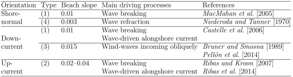
Table 4 shows an alternative classification of transverse bars based on their orientation, 742
an important property that will turn out to depend critically on the DASC profile. The 743
orientation down-current or up-current is sometimes difficult to differentiate in the field 744
as this require the identification of the main forcing, so only the sites where the latter has 745
been identified are included in Table 4. For this, a forcing analysis must be performed if the 746
incoming waves have two dominant directions or in the presence of tidal currents [Pell´on 747
et al., 2014]. The slope of the part of the beach where the bars appear is also indicated 748
in Table 4. The shore-normal large-scale finger bars appear on flat terraces (e.g., slope of 749
0.003). The beach profiles below the shore-normal TBR bars and the down-current bars 750
are similar: gentle-sloping upper (or low-tide) terraces. Up-current bars appear for larger 751
beach slopes (0.02-0.04) in the subtidal zone [Ribas et al., 2014]. 752
5.2. Existing theories for their formation
As occurred for the case of crescentic bars (section 4.2), during the 80’s and the 90’s the 753
formation of rhythmic patches of transverse bars was commonly conceived to be caused 754
by hydrodynamic template models, in which rhythmic morphologic patterns are forced 755
solely by edge waves [e.g., Holman and Bowen, 1982]. However, as discussed byCoco and 756
Murray [2007], such theory is hardly consistent with observations by a number of reasons, 757
![TABLE 3.Classification of observed transverse bars, following Pell´on et al. [2014],](https://thumb-us.123doks.com/thumbv2/123dok_us/8678986.378008/117.595.69.561.296.551/table-classication-observed-transverse-bars-following-pell-et.webp)