Analysis of patch test consistent atomistic to continuum coupling with higher order finite elements

warwick.ac.uk/lib-publications

Dedner, Andreas, Ortner, Christoph and Wu, H. (2017) Analysis of patch-test consistent atomistic-to-continuum coupling with higher-order finite elements. ESAIM: Mathematical Modelling and Numerical Analysis, 51 (6). pp. 2263-2288. doi:10.1016/j.epidem.2017.04.001

Permanent WRAP URL:

http://wrap.warwick.ac.uk/87419

Copyright and reuse:

The Warwick Research Archive Portal (WRAP) makes this work by researchers of the University of Warwick available open access under the following conditions. Copyright © and all moral rights to the version of the paper presented here belong to the individual author(s) and/or other copyright owners. To the extent reasonable and practicable the material made available in WRAP has been checked for eligibility before being made available.

Copies of full items can be used for personal research or study, educational, or not-for-profit purposes without prior permission or charge. Provided that the authors, title and full

bibliographic details are credited, a hyperlink and/or URL is given for the original metadata page and the content is not changed in any way.

Publisher’s statement:

“Reproduced with permission from © EDP ”.

A note on versions:

The version presented here may differ from the published version or, version of record, if you wish to cite this item you are advised to consult the publisher’s version. Please see the ‘permanent WRAP URL’ above for details on accessing the published version and note that access may require a subscription.

ATOMISTIC-TO-CONTINUUM COUPLING WITH HIGHER-ORDER FINITE ELEMENTS

A. S. DEDNER, C. ORTNER, AND H. WU

Abstract. We formulate a patch test consistent atomistic-to-continuum coupling

(a/c) scheme that employs a second-order (potentially higher-order) finite element method in the material bulk. We prove a sharp error estimate in the energy-norm, which demonstrates that this scheme is (quasi-)optimal amongst energy-based sharp-interface a/c schemes that employ the Cauchy–Born continuum model. Our analysis also shows that employing a higher-order continuum discretisation does not yield qualitative improvements to the rate of convergence.

1. Introduction

Atomistic-to-continuum (a/c) coupling is a class of coarse-graining methods for efficient atomistic simulations of systems that couple localised atomistic effects de-scribed by molecular mechanics with long-range elastic effects dede-scribed by contin-uum models using the finite-element method. We refer to [6], and references therein for an extensive introduction and references.

The presented work explores the feasibility and effectiveness of introducing higher-order finite element methods in the a/c framework, specifically for quasi-nonlocal (QNL) type methods.

The QNL-type coupling, first introduced in [15], is an a/c method that uses a “geometric consistency condition” [3] to construct the coupling between the atom-istic and continuum model. The first explicit construction of such a scheme for two-dimensional domains with corners is described in [12] for a neareast-neighbour many-body site potential. We call this construction ”G23” for future reference. This approach satisfies force and energy patch tests (often simply called consistency), which in particular imply absence of ghost forces.

We will supply the G23 scheme with finite element methods of different orders and investigate the rates of convergence for the resulting schemes. Our conclusion will be that second-order finite element schemes are theoretically superior to first-order schemes, while schemes of third and higher first-order do not improve the rate of convergence. This conclusion is independent of defect types, since the total error can only be as good as the Cauchy–Born modeling error in the continuum region, which is of second order, just as a P2-finite element method. We further find that the consistency error of the a/c scheme is in fact dominated by the coupling component of the modelling error. Because of all these limitations, we will explore, for a basic

Date: March 16, 2017.

Key words and phrases. atomistic models, coarse graining, atomistic-to-continuum coupling, quasicontinuum method, error analysis.

HW was supported by MASDOC doctoral training centre, EPSRC grant EP/H023364/1. CO was supported by ERC Starting Grant 335120.

model problem, how well second-order schemes fare in practise against first-order schemes.

1.1. Outline. The theory of high-order finite element methods (FEM) in partial differential equations, and applications in solid mechanics is well established; see [14] and references therein. However, most work on the rigorous error analysis of a/c coupling has been restricted to P1 finite element methods; the only exception we are aware of is [11], which focuses on blending-type methods.

In the present work we estimate the accuracy of a QNL method employing a P2 FEM in the continuum region against an exact solution obtain from a fully atomistic model. Since stability of QNL type couplings is a subtle issue [9] we will primarily analyse the consistency errors, taking into account the relative sizes of the fully re-solved atomistic region and of the entire computational domain (Sections 6.1-6.6). We will then optimize these relative sizes as well as the mesh grading in the con-tinuum region in order to minimize the total consistency error (Section 6.7). We will observe that, using P1-FEM in the continuum region, the error resulting from FEM approximations is the dominating contributor of the consistency estimates, which implies that increasing the order of the FEM can indeed improve the accu-racy of the simulation. We will show that, using Pk-FEM with k ≥ 2, the FEM approximation error is dominated by the interface error which comes purely from the G23 construction, and in particular demonstrate that the P2-FEM is sufficient to achieve the optimal convergence rate for the consistency error. Finally,assuming

the stability of the G23 coupling (see assumption(A2)in_§3.2, and also [9] why this must be an assumption and cannot be proven), we prove a rigorous error estimate in_§6.

Finally, we conduct numerical experiments on a 2D anti-plane model problem to test our analytical predictions. The numerical results display the predicted error convergence rates for the fully atomistic model, P1-FEM G23 model, and P2-FEM G23 model.

2. Preliminaries

Our setup and notation follows [12]. As our model geometry we consider an infinite 2D triangular lattice,

Λ :=A_Z2, with A=





1 cos(π/3) 0 sin(π/3)



.

We define the six nearest-neighbour lattice directions by a1 := (1,0), and aj :=

Qj6−1a1, j ∈Z, where Q6 denotes the rotation through the angle π/3. We supply Λ

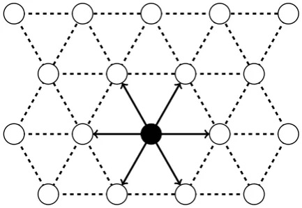
with an atomistic triangulation, as shown in Figure 1, which will be convenient in both analysis and numerical simulations. We denote this triangulation byT and its elements byT ∈ T. We also denote a:= (aj)6j=1, andFa:= (Faj)6j=1, forF∈Rm

×2

. We identify a discrete displacement mapu: Λ_→Rm_{,m= 1,2,3, with its}

continu-ous piecewise affine interpolant, with weak derivative_∇u, which is also the pointwise derivative on each element T _{∈ T}. For m = 1,2,3, the spaces of displacements are defined as

U0 :=

u|Λ→Rm : supp(∇u) is compact , and

˙

U1,2 _:=

Figure 1. The lattice and its canonical triangulation.

We equip ˙_U1,2 _{with theH}1_{-seminorm,kuk}

U1,2 :=k∇uk_L2₍

R2). From [8] we know that

U0 is dense in ˙U1,2 in the sense that, if u∈U˙1,2, then there exist uj ∈ U0 such that ∇uj → ∇u strongly inL2.

A homogeneous displacement is a map uF : Λ → Rm, uF(x) := Fx, where F ∈

Rm×2.

For a map u: Λ→Rm, we define the finite difference operator

Dju(x) :=u(x+aj)−u(x), x∈Λ, j ∈ {1,2, ...,6}, and

Du(x) := (Dju(x))6j=1.

(2.1)

Note thatDuF(x) =Fa.

2.1. 2D many-body nearest neighbour interactions. We assume that the atom-istic interaction is described by a nearest-neighbour many-body site energy potential

V ∈ Cr₍

Rm×6),r ≥5, with V(0) = 0. Furthermore, we assume that V satisfies the point symmetry

V((₋gj+3)j6=1) = V(g) ∀g∈R

m×6 .

The energy of a displacementu_{∈ U}0, given by

Ea_{(u) :=} X

`∈Λ

V(Du(`)),

is well-defined since the infinite sum becomes finite. To formulate a variational problem in the energy space ˙U1,2_{, we need the following lemma to extendE}a _{to ˙U}1,2_.

Lemma 2.1. _Ea : (U0,k∇ · kL2) → _R is continuous and has a unique continuous extension to _U˙1,2_{, which we still denote by E}a_{. Furthermore, the extended E}a _:

( ˙U1,2_{,k∇ · k}

L2)→_R isr-times continuously Fr´echet differentiable.

Proof. See Lemma 2.1 in [4].

2.2. The variational problem. We add an external potential f ∈Cr_{( ˙U}1,2_{) with} ∂u(`)f(u) = 0 for all|`| ≥Rf, whereRf is some given radius, andf(u+c) =f(u) for

all constantsc. For example, we can think of f modelling a substitutional impurity. See also [5, 7] for similar approaches.

We then seek the solution to

ua ∈arg min Ea

(u)−f(u)|u∈U˙1,2

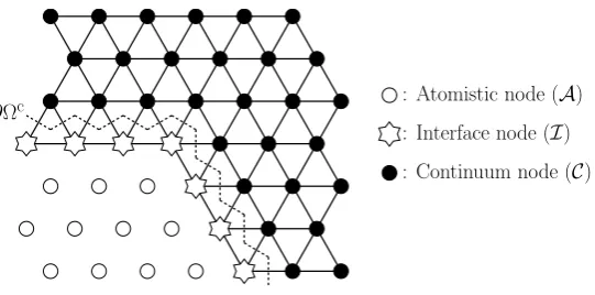
∂Ωc : Atomistic node (A) : Interface node (I)

: Continuum node (_C)

Figure 2. The domain decomposition with a layer of interface atoms.

For u, ϕ, ψ∈U˙1,2 _{we define the first and second variations of E}a _by hδEa_{(u), ϕi:= lim}

t→0t −1

(Ea_{(u+tϕ)− E}a_(u)),

hδ2

Ea_{(u)ϕ, ψ}

i:= lim

t→0t −1

(_hδ_Ea_{(u+tϕ), ψ}

i − hδ_Ea_{(u), ψ} i).

We use analogous definitions for all energy functionals introduced in later sections.

2.3. The Cauchy–Born Approximation. The Cauchy–Born strain energy func-tion, corresponding to the interatomic potentialV is

W(F) := 1 Ω0

V(Fa), for F_∈Rm×2,

where Ω0 := √

3/2 is the volume of a unit cell of the lattice Λ. Thus W(F) is the energy per volume of the homogeneous latticeFΛ.

2.4. The G23 coupling method. LetA ⊂ Λ denote the set of all lattice sites for which we want to maintain full atomistic accuracy. We denote the set of interface lattice sites by

I :=

`_∈Λ_{\ A}

`+a_j ∈ A for some j ∈ {1, . . . ,6}

and we denote the remaining lattice sites byC := Λ\(A ∪ I). Let Ω` be the Voronoi

cell associated with site`. We define the atomistic, interface and continuum regions respectively by

Ωa _:= [

`∈A

Ω`, Ωi:=

[

`∈I

Ω`, and Ωc:=R2\

[

`∈A∪I

Ω`;

see Figure 2 for a visualisation.

A general form for the GRAC-type a/c coupling energy [3, 12] is

Eac_{(u) =}X

`∈A

V(Du(`)) +X

`∈I

V (_R`Dju(`))6j=1

+

Z

Ωc

W(_∇u(x)) dx,

where_R`Dju(`) :=P6i=1C`,j,iDiu(`). The parametersC`,j,i are to be determined in

order for the coupling scheme to satisfy the “patch tests”:

Eac _{is locally energy consistent if, for all F∈}

Rm×2,

V<sub>`</sub>i(Fa) =V(Fa) <sub>∀</sub>`_{∈ I}. (2.3)

Eac _{is force consistent if, for all F∈}

Rm×2,

δEac_(u

A

3

C

A

3

C

A C

7

Figure 3. The first two configurations are allowed. The third configu-ration is not allowed as the interface atom at the corner has no nearest neighbour in the continuum region, and should instead be taken as an atomistic site.

2 3 2

3 2 3 2

3

2 3

2 3

2 3

1

1

1

1

1

1

1

1

1

1

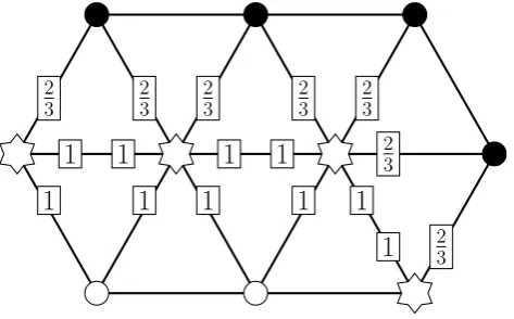
Figure 4. The geometry reconstruction coefficents λx,j at the interface sites.

Eac _{is patch test consistent if it satisfies both (2.3) and (2.4).}

For the sake of brevity of notation we will often writeVi

`(Du(`)) :=V (R`Dju(`))6j=1

. Following [12] we make the following standing assumption (see Figure 3 for exam-ples).

(A0)Each vertex`∈ I has exactly two neighbours in_I, and at least one neighbour in _C.

Under this assumption, the geometry reconstruction operator R` is then defined

by

R`Djy(`) := (1−λ`,j)Dj−1y(`) +λ`,jDjy(`) + (1−λ`,j)Dj+1y(`),

λx,j :=

 



2/3, x+aj ∈ C

1, otherwise ;

see Figure 4. The resulting coupling method is called G23 and the corresponding energy functional Eg23_{. This choice of coefficients (and only this choice) leads to}

patch test consistency (2.3) and (2.4).

For future reference we decompose the canonical triangulation T as follows:

TA : ={T ∈ T |T ∩(I ∪ C) =∅}, TC : ={T ∈ T |T ∩(I ∪ A) =∅} and TI : =T \(TC∪ TA).

2.5. Notation for a P2 finite element scheme. In the atomistic and interface regions, the interactions are represented by discrete displacement maps, which are identified with their linear interpolant. Here, we identify the displacement map with its P1 interpolant. No approximation error is committed.

On the other hand, in the continuum region where the interactions are approxi-mated by the Cauchy–Born energy, we could increase the accuracy by using Pp-FEM with p > 1. In later sections we will review that the Cauchy–Born approximation yields a 2nd-order error, whereas employing the P1-FEM in the continuum region would reduce the accuracy to first order. In fact, we will show in that, with opti-mized mesh grading, P2-FEM is sufficient to obtain a convergence rate that cannot be improved by other choices of continuum discretisations. High-order Pp-FEM with

p > 2 will increase the computational costs but yield the same error convergence rate (see _§ 3.5).

Let K >0 denote the inner radius of the atomistic region,

K := sup

r >0| Br∩Λ⊂ A ,

where _Br denotes the ball of radius r centred at 0. In order for the defect to be

contained in the atomistic region we assume throughout thatK _≥Rf.

Let Ωh denote the entire computational domain and N > 0 denote the inner

radius of Ωh, i.e.,

N := sup

r >0| Br ⊂Ωh .

LetTh be a finite element triangulation of Ωh which satisfies that, for T ∈ Th, T is

closed and

T ∩(A ∪ I)6=∅ ⇒ T ∈ T.

In other words,Th andT coincide in the atomistic and interface regions, whereas in

the continuum region the mesh size may increase towards the domain boundary. The optimal rate at which the mesh size increases will be determined in later sections.

We note that the concrete construction of Th will be based on the choice of the

domain parameters K and N; hence, when emphasizing this dependence, we will write_Th(K, N). We assume throughout that the family (Th(K, N))K,N is uniformly shape-regular, i.e., there exists c > 0 such that,

diam(T)2

≤c_|T_|, _∀T _{∈ T}h(K, N),∀K ≤N. (2.6)

This assumption eliminates the possibility of extreme angles on elements, which would deteriorate the constants in finite element interpolation error estimates. For the most part we will again drop the parameters from the notation by writing

Th ≡ Th(K, N) but implicitly will always keep the dependence.

Similar to (2.5), we define the atomistic, interface and continuum elements as

Ta

h,Thi and Thc, respectively. Note that Tha = TA and T_hi = TI. We also let Nh

denote the number of degrees of freedom of _Th.

We define the finite element space of admissible displacements as

Uh :=

u_∈C(R2;Rm)| supp(u)⊂Ωh, u|T ∈P1(T) for T ⊂ Tha∪ Thi and

u_|T ∈P2(T) forT ⊂ Thc .

(2.7)

In defining _Uh we have made two approximations to the class of admissible

The computational scheme is to find

ug23_h ∈arg min Eg23_(u

h)−f(uh)|uh ∈ Uh . (2.8)

Remark 2.2. _Uh is embedded in U0 via point evaluation. Through this

identifi-cation,f(uh) is well-defined for alluh ∈ Uh.

We will make this identificationonlywhen we evaluate f(uh). The reason for this

is a conflict when interpreting elements uh as lattice functions is that we identify

lattice functions with their continuous interpolants with respect to the canonical triangulation_T, which would be different from the function uh itself. However, for

the evaluation off(uh) this issue does not arise.

3. Summary of results

3.1. Regularity of ua_{. The approximation error analysis in later sections requires}

estimates on the decay of the elastic fields away from the defect core. These results follow from a natural stability assumption:

(A1) The atomistic solution is strongly stable, that is, there exists C0 >0,

hδ2

Ea_(ua_{)ϕ, ϕ}

i ≥C0_k∇ϕ_k2

L2, ∀ϕ∈U˙1,2, (3.1)

whereua _{is a solution to (2.2).}

Corollary 3.1. Suppose that (A1) is satisfied, then there exists a constant C > 0

such that, for 1_≤j _≤r₋2,

|Djua(`)| ≤C|`|−1−j_.

Proof. See Theorem 2.3 in [4].

3.2. Stability. In [9] it is shown that there is a “universal” instability in 2D inter-faces for QNL-type a/c couplings: it is impossible to prove in full generality that

δ2_Eg23_(ua_{) is a positive definite operator, even if we assume (3.1). Indeed, this}

po-tential instability is universal to a wide class of generalized geometric reconstruction methods. However, it is rarely observed in practice. To circumvent this difficulty, we make the following standing assumption:

(A2) The homogeneous lattice is strongly stable under the G23 approximation, that is, there existsC0g23 >0 which is independent ofK such that, forK sufficiently

large,

hδ2

Eg23_(0)ϕ

h, ϕhi ≥C0g23k∇ϕhk 2

L2, ∀ϕh ∈ Uh. (3.2)

3.3. Main results. To state the main results it is convenient to employ a smooth interpolant to measure the regularity of lattice functions. In Lemma 6.1, we define such an interpolant ˜u ∈ C2,1₍

R2) for u ∈ U0, for which there exists a universal

constant ˜C such that, for all q_∈[1,_∞], 0_≤j _≤3,

|Dju(`)| ≤C˜k∇j_u˜k L1_(ω

`) and k∇ j_u˜k

Lq_(T) ≤C˜kDjuk_`q_(Λ∩T)

whereω` :=`+A(−1,1)2.

3.3.1. Consistency error estimate. In (5.6) we define a quasi-best approximation operator Πh : U0 → Uh, which truncates an atomistic displacement to enforce the

homogeneous Dirichlet boundary condition, and then interpolates it onto the finite element mesh.

Our main result is the following consistency error estimate.

Theorem 3.2. If ua _{is a solution to (2.2) then we have, for all ϕ}

h ∈ Uh,

hδ_Eg23_(Π

hua), ϕhi.

k∇2_u˜a

kL2_(Ωi₎+k∇3u˜ak_L2_(Ωc₎+k∇2u˜ak2_L4_(Ωc₎

+_kh2 ∇3_u˜a

kL2_(Ωc

h)+k∇u˜ a

kL2₍

R2\BN/2)

+N−1kh2∇2

˜

uakL2_(B

N\BN/2)

k∇ϕhkL2₍

R2\Ωa),

(3.3)

where Ωc

h corresponds to the continuum region of Ωh, and h(x) := diam(T) with

x∈T ∈ Th.

3.3.2. Optimizing the approximation parameters. Before we estimate the error_k∇ua₋ ∇uhkL2, we optimize the approximation parameters in the computational scheme.

This means that the radius K of the atomistic region, the radius N of the entire computational domain and the mesh sizehshould satisfy certain balancing relations. We only outline the result of this optimisation and refer to § 6.7 for the details.

Due to the decay estimates on ˜ua _{the dominating terms in (3.3) turn out to be} k∇2_u˜a_k

L2_(Ωi₎ and k∇u˜ak_L2₍

R2\BN/2). (3.4)

(We will see momentarily that the mesh size plays a minor role.) These two terms result from the nature of the coupling scheme and the far-field truncation error. In particular, both of these cannot be improved by the choice of discreti-sation of the Cauchy–Born model, e.g., order of the FEM. We also note that, if we had employed a P1-FEM, the only different terms in the analog of (3.3) are

kh∇2_u˜a_k

L2_(Ωc₎ rather than kh2∇3u˜ak_L2_(Ωc₎, and N−1kh∇u˜ak_L2_(B

N\BN/2) rather than N−1

kh2_∇2_u˜a_k

L2_(B

N\BN/2), hence the limiting factor would have beenkh∇ 2_u˜a_k

L2_(Ωc₎.

We can balance the two terms in (3.4) by choosing N ≈K5/2_{. It then remains to}

determine a mesh-size so that the finite element error contribution,

kh2_∇3_u˜a_k

L2_(Ωc

h) and N

−1

kh2_∇2_u˜k

L2_(B

N\BN/2)

remains small in comparison. We show that the scaling h(x)≈|Kx|

β

is a suitable choice, with 1< β < 3/2, under which both terms become of order O(K−3_).

β N Nh consistency error

P2-FEM 1,3 2

K5/2 _K2 _K−5/2

P1-FEM 1,3 2

K2 _K2 _K−2

Table 1. Quasi-optimal relations between approximation parameters

for P2-GR23 and, for comparision, for P1-GR23.

Corollary 3.3. Suppose that N, h satisfy the relations of Table 1, the consistency error estimate (3.3) in terms of the number of degrees of freedom _Nh can be written as

kδEg23

(Πhua)kU−1,2 .N_h−5/4. (3.5)

3.3.3. Error estimate. To complete our summary of results, we now use the Inverse Function Theorem to obtain error estimates for the strains and the energy.

Theorem 3.4. Suppose that (A0), (A1) and (A2) are satisfied and that the quasi-optimal scaling of N, h from Table 1 is satisfied. Then, for sufficiently large atomistic region sizeK, a solution ug23_h to (2.8) exists which satisfies the error estimates

k∇ua_{− ∇u}g23

h kL2 .N_h−5/4, and (3.6)

[Ea(ua)−f(ua)]−[Eg23(u g23

h )−f(u

g23

)].N −7/4

h , (3.7)

where _Nh is the number of degrees of freedom.

Remark 3.5. The analogous estimates of P1-GR23 to (3.6) and (3.7) are N−1

h

and _Nh−2 respectively.

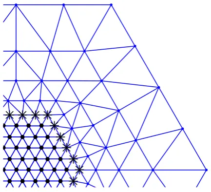
3.4. Setup of the numerical tests. For our numerical tests, we consider an anti-plane displacementu: Λ_→R. We choose a hexagonal atomistic region Ωa _{with side}

length K and one layer of atomistic sites outside Ωa _{as the interface. To construct}

the finite element mesh, we add hexagonal layers of elements such that, for each layer

j, h(layer j) = (_|x_|/K)β_{, with β = 1.4; see Figure 5. The procedure is terminated}

once the radius of the domain exceeds N = dK5/2_{e. This construction guarantees}

the quasi-optimal approximation parameter balance to optimise the P2-FEM error. The derivation is given in Section 6.7.

In our tests we compare the P2-G23 method against

(1) a pure atomistic model with clamped boundary condition: the construction of the domain is as in the P2-G23 method, but without continuum region; (2) a P1-G23 method: the construction is again identical to that of the P2-G23

method, but the P2-FEM in the definition of _Uh is replaced by a P1-FEM.

-15 -10 -5 0 5 10 15 -10

-5 0 5 10

Figure 5. An example of the computatioanl mesh. The the vertices marked by ”_•” are the atomistic sites; the vertices marked by ”_∗” are the interface sites.

The site potential is given by a nearest-neighbour embedded atom toy model,

V(Du) :=G 6 X

i=1

ρ(|Diu(`)|)

!

withG(s) :=s+1 2s

2 _{and ρ(r) := sin}2_{(rπ). This is a simplified anti-plane toy model}

as used in [4], which absorbs the pair interaction into the embedding term.

The external potential is defined by hf, ui = 10(u(0,0)−u(1,0)), which can be thought of as an elastic dipole. A steepest descent method, preconditioned with a finite element Laplacian and fixed (manually tuned) step-size, is used to find a minimizer ug23_h of Eg23_{(u)−f(u), using u}

h = 0 as the starting guess.

In order to compare the errors, we use a comparison solution with atomistic region size 3K and other computational parameters scaled as above.

The numerical results, with brief discussions, are shown in Figures 6–9. The two most important observations are the following:

(1) the numerical tests confirm the analytical predictions for the energy-norm error, but the experimental rates for the energy error are better than the analytical rates. Similar observations were also made in [4].

(2) With our specific setup, the improvement of the P2-GR23 over P1-GR23 is clearly observed when plotting the error against #_{A ∝ N}h, but when

plotted against _Nh the improvement is only seen in the asymptotic regime.

This indicates that further work is required, such as a posteriori adaption, to optimise the P2-GR23 in the pre-asymptotic regime as well.

3.5. Extension to high-order FEM. If we apply higher-order FEM in the contin-uum region, then to extend our error analysis we would need a smooth interpolant of u _{∈ U}0 with higher regularity than ˜u ∈ C2,1(R2). A suitable extension given in

[5] is, for arbitrary n, a Cn,1 _{piecewise polynomial of degree 2n + 1 with}

proper-ties analogous to those stated in Lemma 6.1. The resulting higher-order decay rate

|∇j_u˜a_(x)|

100 101 102 10-5

10-4 10-3 10-2

10-1 Point Defect : Geometry Error

ATM G23-P2 G23-P1

Figure 6. Error in energy norm plotted against #A. We clearly

observe the predicted rate of convergence.

Nh

101 102 103 104 105

k

D

7

uh

!

D

7

u

k`

2

10-5 10-4 10-3 10-2

10-1 Point Defect : Geometry Error

ATM G23-P2 G23-P1

9N!1

h

9Nh!5=4

9_Nh!1=2

Figure 7. Error in energy norm plotted against the number of degrees

100 101 102 10-8

10-7 10-6 10-5 10-4 10-3 10-2

10-1 Point Defect : Energy Error

ATM G23-P2 G23-P1

Figure 8. The energy error plotted against #_A. The observed rate of convergence is better than the rate predicted in Theorem 3.4.

Nh

101 102 103 104 105

j

E

h(

7uh

)

!

E

a(

7

u

a)j

10-8 10-7 10-6 10-5 10-4 10-3 10-2

10-1 Point Defect : Energy Error

ATM G23-P2 G23-P1

9N!1

h

9N!2

h

9N!52

h

However, as we have pointed out in_§3.3.2, if we employ the mesh gradingh(x) = (_|x_|/K)β _{with 1< β < 3/2 in the continuum region, the total approximation error}

cannot be improved by using Pp-FEM withp > 2, since the dominating term is the interface error k∇2_u˜a_k

L2_(Ωi₎ for p ≥ 2, which results from the construction of G23

coupling and is not affected by the choice of FEM.

If we consider a coarser mesh for high-order FEM in hopes of reducing the number of degrees of freedom, i.e., choosing β ≥ 3/2, then applying analogous calculations to those in§6.7 gives us the following result:

Employing Pp-FEM with p > 2, in order to match the convergence rate of the Cauchy–Born error term_k∇3_u˜a_k

L2_(Ωc₎ ∼K−3, the highest mesh coarsening rate is

β = 5 3 −

1 3p.

This means that the optimal mesh grading that Pp-FEM can achieve without compromising accuracy is no greater than 5

3. However, in that case, the number of

degrees of freedom is always _O(K2_).

4. Conclusion

We obtained a sharp energy-norm error estimate for the G23 coupling method with P2-FEM discretisation of the continuum model. Furthermore, we demonstrated that, with P1-FEM discretisation the FEM coarsening error is the dominating term in the consistency error estimate, whereas for P2-FEM discretisation the interface error becomes the dominating term. In particular, a P2-FEM discretisation yields a more rapid decay of the error. Crucially though, since for Pp-FEM with p _≥ 2 the interface contribution dominates the total error the P2-FEM is already optimal. That is, increasing to p > 2 will not improve the rate of convergence, but increase the computational cost and algorithmic complexity.

Numerically, we observe that the improvement of P2-GR23 over P1-GR23 is only modest at moderate _Nh, hence a P2-GR23 scheme would be primarily of interest

if very high accuracy of the solution is required. Purely according to our a priori

error analysis, considering the additional algorithmic complexity, it is unclear how practically useful higher-order FEM in the context of A/C coupling are. However, before drawing such a universal conclusion, one should explore whether optimis-ing the pre-asymptotic regime, usoptimis-ing hp a posteriori mesh adaption, could lead to improved cost/error rates.

While our estimates for the error in energy-norm are sharp, our numerical results show the estimates for the energy errors are suboptimal. We hightlight the leading term in the error analysis which overestimate the error in Section 7.2. We are unable, at present, to obtain an optimal energy error estimate. This appears to be an open problem throughout the literature on hybrid atomistic multi-scale schemes; see e.g. [4].

5. Reduction to consistency

Assuming the existence of an atomistic solution ua_{, we seek to prove the existence}

of ug23_h ∈ Uh satisfying

hδ_Eg23_(ug23

h ), ϕhi=hδf(u

g23

h ), ϕhi, for all ϕh ∈ Uh, (5.1)

and to estimate the kua_−ug23

h kin a suitable norm.

The error analysis consists of consistency and stability estimates. Once these are established we apply the following theorem to obtain the existence of a solutionug23_h

and the error estimate. The proof of this theorem is standard and can be found in various references, e.g. [13, Lemma 2.2].

Theorem 5.1 (The inverse function theorem). Let _Uh be a subspace of U, equipped with_{k∇ · k}L2, and let G_h ∈C1(U_h,U_h∗)with Lipschitz-continuous derivative δGh:

kδ_Gh(uh)−δGh(vh)kL≤Mk∇uh− ∇vhkL2 for all u_h, v_h ∈ U_h, where _{k · k}L denotes the L(Uh,Uh∗)-operator norm.

Let u¯h ∈ Uh satisfy

kGh(¯uh)kU∗

h ≤η, (5.2)

hδGh(¯uh)vh, vhi ≥γk∇vhk2L2 for all vh ∈ Uh, (5.3) such that M, η, γ satisfy the relation

2M η γ2 <1.

Then there exists a (locally unique)uh ∈ Uh such that Gh(uh) = 0,

k∇uh− ∇u¯hkL2 ≤2η

γ, and

hδ_Gh(uh)vh, vhi ≥

1₋ 2M η

γ2

γ_k∇vhk2L2 for all v_h ∈ U_h.

To ensure Dirichlet boundary conditions, we adapt the quasi-best approximation map defined in [4]. Letµ∈C3₍

R2) be a cut-off function such that

µ(x) =

 



1 0≤x≤ 1 2,

0 x_≥1.

Foru: Λ_→Rm, define

Lu(x) := µ

|x| N

(˜u(x)−au), where au :=

1

|BN \BN/2| Z

BN\BN/2

˜

u(y) dy. (5.4)

Let νT,i, i = 1,2,3 be the vertices of T and me be the mid-point of an edge e.

Then, the set of allactive P2 finite element nodes is given by

Nh :={νT,i|T ∈ Th, i= 1,2,3} ∪ {me|e=T1∩T2, T1, T2 ∈ Thc}.

Furthermore, let I2

h : C(R2;Rm) → Uh be the interpolation operator such that,

for g _∈ C(R2;Rm), Ih2(g)|T ∈ P1(T) for T ⊂ Tha∪ Thi, Ih2(g)|T ∈P2(T) forT ⊂ Thc,

and

I_h2(g)(x) =g(x) for all x∈ Nh.

Remark 5.2. We also introduce ghost nodes on the edges shared by interface and continuum elements:

Nhg :={me|e=T1∩T2, T1 ∈ Thi, T2 ∈ Thc}. (5.5)

Then, for x_{∈ Nh}g, I2

h(g)(x) = (g(νx1) +g(νx2))/2, where νx1 andνx2 are the vertices of

the edge on whichx lies. Hence, the P1 _{and P}2 _{interpolants coincide on N}g

h.

We can now define the projection map (quasi-best approximation operator) Πh : U0 → Uh as

Πh :=Ih2◦ L. (5.6)

5.1. Stability. To put Theorem 5.1 (Inverse Function Theorem) into our context, let

Gh(v) :=δEg23(v)−δf(v) and u¯h := Πhua.

To make (5.2) and (5.3) concrete we will show that there exist η, γ > 0 such that, for all ϕh ∈ Uh,

hδ_Eg23_(Π

hua), ϕhi − hδf(Πhua), ϕhi ≤ηk∇ϕhkL2, (consistency) hδ2

Eg23_(Π

hua)ϕh, ϕhi − hδ2f(Πhua)ϕh, ϕhi ≥γk∇ϕhk2L2. (stability)

Ignoring some technical requirements, the inverse function theorem implies that, if

η/γ is sufficiently small, then there existsug23_h ∈ Uh such that hδ_Eg23_(ug23

h ), ϕhi − hδf(ug23h ), ϕhi= 0, ∀ϕh ∈ Uh, and k∇ug23_{h − ∇}ΠhuakL2 ≤2η

γ.

Finally adding the best approximation error k∇Πhua− ∇uakL2 gives the error

esti-mate

k∇ug23_{h − ∇}ua

kL2 ≤ k∇Π_hua− ∇uak_L2 + 2η γ

The Lipschitz and consistency estimates require assumptions on the bounded-ness of partial derivatives of V. For g _{∈ R}m×6, define the first and second partial derivatives, for i, j = 1, . . . ,6, by

∂jV(g) :=

∂V(g)

∂gj ∈R

m_{, and ∂}

i,jV(g) :=

∂2_V(g) ∂gi∂gj ∈R

m×m_,

and similarly for the third derivatives ∂i,j,kV(g) ∈ Rm×m×m. We assume that the

second and third derivatives are bounded

M2 : =

6 X

i,j=1

sup

g∈Rm×6 sup

h1,h2∈R2,

|h1|=|h2|=1

∂i,jV(g)[h1, h2]<∞, and (5.7)

M3 : =

6 X

i,j,k=1

sup

g∈Rm×6

sup

h1,h2,h3∈R2,

|h1|=|h2|=|h3|=1

∂i,j,kV(g)[h1, h2, h3]<∞. (5.8)

6 X

i=1

|∂iV(g)−∂iV(h)| ≤M2 max

j=1,...,6|gj−hj|, 6

X

i,j=1

|∂i∂jV(g)−∂i∂jV(h)| ≤M3 max

k=1,...,6|gk−hk|, forg,h∈R

m×6

. (5.9)

From the bounds above we can obtain the following Lipschitz continuity and stability results.

Lemma 5.3. There exists M >0 such that

kδ_Gh(uh)−δGh(vh)kL ≤Mk∇uh− ∇vhkL2 for all u_h, v_h ∈ U_h. (5.10)

Proof. The result follows directly from (5.9) and the fact thatf _∈Cr_{( ˙U}1,2_{) and that} δf is compactly supported hence δ2_{f is also Lipschitz. Namely, for allϕ}

h ∈ Uh, h(δGh(uh)−δGh(vh))ϕh, ϕhi

=h(δ2Eg23

(uh)−δ2Eg23(vh))ϕh, ϕhi+h(δ2f(vh)−δ2f(uh))ϕh, ϕhi ≤Cg23M3_k∇uh − ∇vhkL∞k∇ϕ_hk2_L2 +C_fku_h−v_hk_L∞(B_Rf)kϕhk2L2 .k∇uh− ∇vhkL2k∇ϕ_hk2_L2 +k∇uh− ∇vhkL2_(B

Rf)kϕhk 2

L2,

where Cg23 is the constant resulting from the interface reconstruction and the lin-ear elasticity formulation of Cauchy–Born in the continuum region, and Cf is the

Lipschitz constant ofδ2_f.

Lemma 5.4. Under the assumptions(A1)and(A2), if_Gh(v) :=δEg23(v)−δf(v), then there exits γ >0 such that, when K is sufficiently large,

hδ_Gh(Πhua)ϕh, ϕhi ≥γk∇ϕhk2L2 for all ϕh ∈ Uh. (5.11)

Proof. The proof of this result is a straightforward adaption of the proof of [5, Lemma 4.9], which is an analogous result for blending-type a/c coupling.

6. Consistency estimate with a P2-FEM

6.1. Outline of the consistency estimate. We begin by decomposing the con-sistency error into

hδEg23

(Πhua), ϕhi − hδf(Πhua), ϕhi=

hδEg23

(Πhua), ϕhi − hδEa(ua), ϕi

+{hδf(Πhua), ϕhi − hδf(ua), ϕi}

=:ηint+ηext, (6.1) whereϕh ∈ Uh is given and we can chooseϕ∈ U0 arbitrarily.

For ϕh ∈ Uh, ϕh|T ∈ P2(T) for T ∈ Thc. But the test function ϕ in hδEa(ua), ϕi

where _I+ _{is an extra layer of atomistic sites outside I. With this assumption in}

place, we can further decompose ηint into the following parts,

ηint =

Z

Ωc

∂FW(∇u˜a) : (∇ϕh− ∇ϕ)

+

Z

Ωc

(∂FW(∇Πhua)−∂FW(∇u˜a)) :∇ϕh

+

Z

Ωc

∂FW(∇u˜a)−∂FW(∇ua)

:∇ϕ

+_hδ_Eg23_(ua₎

−δ_Ea_(ua_{), ϕ} i

=:δ1+δ2+δ3+δ4,

(6.2)

where ˜ua _{is the smooth interpolant of u}a _{defined in Lemma 6.1 below. By ∇ϕ in} δ1 we mean the gradient of the canonical linear interpolant of ϕ. To estimate δ2 we require an approximation error estimate for Πhu−u. To estimate δ3 we will exploit

the fact that the atomistic triangulationT is uniform to prove a super-convergence estimate. Finally, for the modelling error, δ4, we employ the techniques developed in [12].

To define the smooth interpolant ˜ua_{, we use the construction from [5], namely a} C2,1_{-conforming multi-quintic interpolant. Although the interpolant defined in [5] is}

for lattice functions onZ2, we can use the linear transformation fromZ2 to Λ = AZ2

to obtain a modified interpolant.

Lemma 6.1. (a) For each u : Λ _{→ R}m_{, there exists a unique u˜ ∈ C}2,1₍

R2;Rm) such that, for all `_∈Λ,

˜

u|`+A(0,1)2 is a polynomial of degree 5,

˜

u(`) =u(`), ∂aiu˜(`) =

1

2(u(`+ai)−u(`−ai)), ∂2

aiu˜(`) =u(`+ai)−2u(`) +u(`−ai), where i_{∈ {}1,2_} and ∂ai is the derivative in the direction of ai.

(b) Moreover, for q∈[1,∞], 0≤j ≤3, k∇j_u˜k

Lq_{(`+A(1,0)</sub>2<sub>)</sub> .kDjuk<sub>`}q<sub>(`+A{−1,0,1,2}</sub>2<sub>)</sub> and |Dju(`)|.k∇ju˜k_L1_(`+A(−1,1)2),

(6.3)

where D is the difference operator defined in (2.1). In particular, k∇u˜_kLq .k∇uk_Lq .k∇u˜k_Lq,

where u is identified with its piecewise affine interpolant.

Proof. Let v :Z2 →Rm and v(ξ) :=u(Aξ) for all ξ∈ Z. Then [5, Lemma 1] shows

that there exists a unique ˜v _∈C2,1₍

R2;Rm) such that, for ξ ∈Z2,

˜

v|ξ+(0,1)2 is a polynomial of degree 5,

˜

v(ξ) =v(ξ), ∂eiv˜(ξ) =

1

2(v(ξ+ei)−v(ξ−ei)), ∂2

eiv˜(ξ) =v(ξ+ei)−2v(ξ) +v(ξ−ei) i= 1,2,

For part (b), [5, Lemma 1] establishes also that there exists a constant C0

j such

that, forξ ∈Z2, 1≤j ≤3, q∈[1,∞],

k∇jv˜_kLq_(ξ+(1,0)2₎ ≤C_j0kDˆjvk_`q_{(ξ+{−1,0,1,2}}2),

where ˆD represents the 4-stencil difference operator in Z2: let R:={ρ ∈Z2| |ρ| =

1}, then ˆDv(`) := ( ˆDρv(`))ρ∈R with ˆDρv(`) := v(`+ρ)−v(`). After transformation,

we have, for ξ=A` ∈Λ,

ˆ

Dv(`) = (Diu(ξ))i=1,2,4,5.

By adding the additional stencil elementsD3, D6 we obtain

C_j00k∇j_u˜k

Lq_(ξ+A(1,0)2₎≤ k∇jv˜k_Lq_(`+(1,0)2₎ ≤C0

jkDˆjvk`q<sub>(`+{−1,0,1,2}</sub>2₎ ≤C_j000kDjuk_`q_{(ξ+A{−1,0,1,2}}2₎,

where C00

j and Cj000 only depend on j. Writing C := max1≤j≤3 _C000

j C00

j

yields the first inequality of (6.3). Following a similar argument the second inequality also

holds.

6.2. Construction of ϕ and estimation of δ1. Recall that

δ1 :=

Z

Ωc

∂FW(∇u˜a) : (∇ϕh− ∇ϕ).

We adapt the modified quasi-interpolation operator introduced in [2] to approxi-mate a test function ϕh ∈ Uh. The advantage of this interpolation operator is that

by using the setting of a partition of unity the approximation error has a local aver-age zero. Consequently we can apply Poincar´e inequality on patches to obtain local estimates.

We think of the construction of ϕ as a Dirichlet boundary problem with the outer boundary ∂Ωh and the inner boundary ∂Ωc. Let φ` be the piecewise linear

hat-functions on the canonical triangulation _T associated with` _∈Λ. Define

φPU

` :=

φ`

P

k∈C∩Ωhφk

, _∀`_{∈ C},

whereC is the continuum lattice sites as defined in§2.4. It is clear that{φPU

` }`∈C∩Ωh

is a partition of unity.

Now we refer to [2] for the contruction of a linear interpolant of ϕh ∈ Uh . We

shall define the interpolant as follows:

where

ϕ1(`) :=

 



ϕh(`), `∈ A ∪ I ∪ I+,

R

R_R2φ`ϕh

R2φ`

, `_{∈ C \ I}+_,

ϕ1(x) :=X

`∈Λ

ϕ1(`)φ`(x), ∀x∈R2,

ϕ2(`) :=

 



R

R2(ϕh−ϕ1)φ

PU `

R

R2φ`

, `∈ C \ I+_,

0, `_{∈ A ∪ I ∪ I}+_,

ϕ2(x) :=X

`∈Λ

ϕ2(`)φ`(x), ∀x∈R2.

Observe that ϕh and ϕboth are supported on a finite domain, hence we can use

Theorem 3.1 in [2] to conclude that

k∇ϕ_kL2_(R2₎ .k∇ϕ_hk_L2_(R2₎, ∀ϕ_h ∈ U_h.

Let g :=−div [∂FW(∇u˜a)]. Then

δ1 =

Z

Ωc

g·(ϕh−ϕ) dx=

Z

Ωc

g·((ϕh−ϕ1)−ϕ2) dx

Sinceϕ2 is a piecewise-linear quasi-interpolant ofϕh−ϕ1 as defined in [2], a direct

consequence of Theorem 3.1 in [2] is that there exists C > 0 such that, recalling Ωa

h :=

S Ta

h,

δ1 ≤Ck∇(ϕh−ϕ1)kL2₍

R2\Ωah)

X

`∈C∩Ωh d2<sub>`</sub>

Z

w`

φPU<sub>`</sub> |g− hgi`|2dx

!1/2 ,

where w` := supp(φ`), hgi` := 1/|w`|R_w

`g(x) dx and d` := diam(w`) = 1. With the

sharp Poincar´e constant derived by [1] , we have

Z

w`

φPU` |g− hgi`|2dx≤

Z

w`

|g− hgi`|2dx≤ <sub>4</sub>1d2`k∇gk2L2_(w `).

On the other hand,ϕ1 is a standard quasi-interpolant of ϕh inSThc, which implies

that there existsC0 _{>0 such that} k∇(ϕh−ϕ1)kL2₍

R2\Ωah) ≤C 0

k∇ϕhkL2₍

R2\Ωah). (6.5)

Due to the fact that d` = 1 and that each point in R2\Ωah is covered by at most

threew`, we have

δ1 ≤Cmax

` d

2

`k∇gkL2₍

R2\Ωah)k∇ϕhkL2(R2\Ωah) ≤CM2_k∇3_u˜a

kL2₍

R2\Ωah)+M3k∇ 2_u˜a

k2

L4₍

R2\Ωah)

k∇ϕhkL2₍

R2\Ωah), (6.6)

where we used the following estimate, for some c >0,

k∇g_kL2_(Ω

h)=k∇div[∂FW(∇u˜ a_)]

kL2_(R2_\Ωa h)

=k∇ ∂F2W(∇u˜

a

)∇2

˜

ua

kL2_(R2_\Ωa h)

= ∂

2

FW(∇u˜

a₎

∇3_u˜a_+∂3

FW(∇u˜

a₎

∇2_u˜a2

L2_(R2_\Ωa h) ≤cM2_k∇3_u˜a

kL2₍

R2\Ωah)+M3k∇ 2_u˜a

k2

L4₍

R2\Ωah)

employing the global bounds (5.7) and (5.8). This completes the estimate for δ1.

6.3. Estimation of δ2. Recall that

δ2 :=

Z

Ωc

(∂FW(∇Πhua)−∂FW(∇u˜a)) :∇ϕh.

We start with estimating the best approximation error.

Lemma 6.2. Let T ∈ Tc

h, u∈U˙1,2 and v ∈W3,2(R2). Then we have the following estimates.

(a) Denote hT := diam(T), then

k∇v− ∇I2

hvkL2_(T) .h2_Tk∇3vk_L2_(T).

(b) There exists a constant C >0 such that, for any domain S ⊃ BN,

k∇Lu− ∇u˜kL2_(S) ≤Ck∇u˜k L2_(S\B

N/2), where _L is the cut-off function defined by (5.4).

(c) Furthermore, we have the best approximation error estimate

k∇Πhu− ∇u˜kL2_(Ωc₎.kh2∇3u˜ak_L2_(Ωc

h)+k∇u˜ a

kL2₍

R2\BN/2)

+N−1kh2_∇2_u˜k

L2_(B

N\BN/2),

(6.7)

where h(x) := diam(T) with x∈T.

Proof. Recall the uniform shape regularity assumption (2.6). Part (a) follows directly from the Bramble–Hilbert Lemma.

For Part (b), we use a variation of Theorem 2.1 in [10]. Applying Poincar´e’s inequality gives

k∇L(u)_{− ∇}u˜_kL2_(S) =

N−1µ0(˜u₋a) + (µ₋1)_∇u˜

L2_(S)

≤N−1Cµku˜−akL2_(S)+k(1−µ)∇u˜k_L2_(S\B N/2) ≤CpCµk∇u˜kL2_(BN\B

N/2)+k(1−µ)∇u˜kL2(S\BN/2) ≤C_k∇u˜_kL2_(S\B

N/2).

For Part (c), we combine Part (a) and (b), that is

k∇Πhu− ∇u˜kL2_(Ωc₎ ≤ k(I_h2◦ L)(u)− L(u)k_L2_(Ωc₎+kL(u)−u˜k_L2_(Ωc₎ .kh2_∇3_L(u)k

L2_(Ωc₎+k∇u˜k_L2_(Ωc_\B N/2)

=

h2 3 X

n=0

1

Nn∇ n_µ

∇3−n(˜u₋a)

L2_(B N\Ωa)

+_k∇u˜_kL2_(R2_\B N/2)

.kh2_∇3_u˜k

L2_(Ωc

h)+k∇u˜kL2(R2\BN/2)+

1

Nkh 2_∇2_u˜k

L2_(B

N\BN/2).

The last line only contains the terms with n = 0,1. The term for n = 2 is

N−2

kh2_∇u˜k

L2_(B

N\BN/2), but since N

−2_h2 _{.1 this is absorved into k∇u˜k}

L2₍

R2\BN/2).

The estimate forδ2 is now a consequence of the best approximation error estimate:

δ2 ≤ k∂FW(∇Πhua)−∂FW(∇u˜a)kL2_(Ωc₎k∇ϕ_hk_L2_(Ωc₎ ≤M2k∇Πhua− ∇u˜akL2_(Ωc₎k∇ϕ_hk_L2_(Ωc₎

.kh2 ∇3_u˜a

kL2_(Ωc

h)+k∇u˜ a

kL2_(R2_\B

N/2) +N −1

kh2 ∇2_u˜

kL2_(B

N\BN/2)

k∇ϕhkL2_(Ωc).

(6.8)

6.4. Estimation of δ3. Recall that

δ3 =

Z

Ωc

∂FW(∇u˜a)−∂FW(∇ua)

:_∇ϕ,

where ϕ is a lattice function with compact support and ∇ϕ denotes the gradient of its piecwise linear interpolant. To estimate this term we observe that ua _{can be}

interpreted as the P1 nodal interpolant of ˜ua_{. Although this indicates a first-order}

estimate only, we can exploit mesh regularity to obtain a second-order superconver-gence estimate.

To that end, we rewrite the integral over the domain as a summation of elements. Let ˚E be the union of edges that are shared by two continuum elements, andωe be

the union of said elements, i.e., ˚

E : ={e=T1∩T2|T1, T2 ∈ TC}. ωe : =T1∪T2, whereT1∩T2 =e.

Recall thatW(F)_≡ 1

Ω0V(F·a). Observe that for a pair of T1, T2 sharing a common

edge e which has the direction of aj, ∇ajϕ(T1) = ∇ajϕ(T2), which allows us to

re-group integration over elements as integration of patches ωe except for elements

near the interface. After simplifying the notation by writing ˜Vj :=∂jV(∇u˜·a) and

Vj :=∂jV(∇u·a), we can rewrite δ3 as follows:

δ3 = 1 Ω0

X

T∈T_C∪T_I 6 X

j=1 Z

T∩Ωc ˜

Vj−Vj

· ∇ajϕ(T)

= 1 Ω0 6 X j=1 X

e∈_E˚_j Z

ωe _˜

Vj−Vj

· ∇ajϕ

+ 1 Ω0

X

T∈T_C∪T_I 6 X

j=1 cT,j

Z

T∩Ωc ˜

Vj−Vj

· ∇ajϕ(T)

=:τ1+τ2,

where ˚Ej :={e∈E˚|e is in the direction of aj} and cT,j is defined as follows,

cT,j =

 



0, ∃e∈E˚j∩T,

1, otherwise.

Observe that for T _{∈ T}C, cT,j is only non-zero near the interface. So we have

τ2 ≤ 1

Ω0 Z

Ωi +

M2|∇u˜a− ∇ua| |∇ϕ|.k∇2

˜

uakL2_(Ωi

ν

ν

T

T

m

ν

ν

a

Figure 10.

where Ωi

+ := S

{T _{∈ T}C|dist(T,Ωi)≤1/2}. Note that the second-order error ∇2u˜a

results from the fact thatua_{is a piecewise linear nodal interpolant of ˜u}a_{on a uniform}

mesh.

To estimate τ1, we employ the following second-order mid-point estimate.

Lemma 6.3. Supposef _∈W2,∞_(T1

∪T2;R) where T1, T2 ∈ T such that they share an edge e and let me be the mid-point of e, then

Z

T1∪T2

f(ξ)₋f(me) dξ

.k∇

2_f

kL∞(T1∪T2).

Then we can write

τ1 = 1 Ω0

6 X

j=1 X

e∈_E˚_j Z

ωe h

( ˜Vj −V˜j(me))−(Vj −V˜j(me))

i

· ∇ajϕ. (6.10)

By Lemma 6.3 we have

Z

ωe

˜

Vj−V˜j(me)

.k∇

2_∂

jV(∇u˜a·a))kL∞(ωe)

. M3k∇2

˜

uak2

L∞(ωe)+M2k∇ 3

˜

uakL∞_(ωe)

.k∇2_u˜a_k2

L4_(ωe)+k∇3u˜akL2_(ω

e), (6.11)

where the last line comes from the fact that ˜ua _{is a polynomial of degree 5 on each} T, hence on each patch ωe the norms are equivalent.

On the other hand, for i= 1, ...6 we denoteνT,i and νT,i0 as the vertices ofT with

νT,i+ai =νT,i0. Then onT ⊃e, we have, using Taylor expansion,

∇ua

|T ·ai− ∇u˜a(me)·ai = ˜ua(νT,i0)−u˜a(νT,i)− ∇u˜a(me)·ai =τe,

where|τe| . k∇3u˜akL∞(ωe). Then for T1 and T2 with T1 ∩T2 = e = [νT,i, νT,i0], we

have

[∇ua_(T1)·a

i− ∇u˜a(me)·ai] + [∇ua(T2)·ai− ∇u˜a(me)·ai] = 2τe.

Z

ωe

Vj−V˜j(me)

=

|T1|(Vj|T1 −V˜j(me)) +|T2|(Vj|T2 −V˜j(me))

=|T1|

6 X

i=1

∂j,iV(∇u˜a(me)·a)

h

∇ua|T1 ·ai− ∇u˜ a

(me)·ai

+∇ua_|

T2 ·ai− ∇u˜ a_(m

e)·ai

i

+O M3k∇2

˜

uak2

L∞(ωe)

.M2k∇3_u˜a_k

L∞(ωe)+M3k∇ 2_u˜a_k2

L∞(ωe).

Combining this estimate with (6.11), we have

τ1 .nk∇2_u˜a k2

L4_(Ωc₎+k∇3u˜ak_L2_(Ωc₎ o

k∇ϕ_kL2_(Ωc).

Finally, combining the last estimate with (6.9) we obtain

δ3 .nk∇2

˜

uakL2_(Ωi

+)+k∇ 2

˜

uak2

L4_(Ωc₎+k∇3u˜akL2_(Ωc₎ o

k∇ϕkL2_(Ωc). (6.12)

6.5. Estimation ofδ4. We observe thatδ4requires the estimation of pure modelling errors regardless of the choice of finite element approximation or domain truncation. This term was the main focus of [12], where the following result was proven.

Theorem 6.4 (Theorem 5.1 [12]). Let u : Λ → Rm and let ϕ : Λ → Rm with compact support, then

hδ_Eg23_(ua₎

−δ_Ea_(ua_{), ϕ} i

.

M2kD2uak`2<sub>(I</sub>ext<sub>)</sub>+M2kD3uak<sub>`</sub>2_(C)+M3kD2uak2_`4_(C)

kDϕk`2(Λ\A),

where _Iext _{:={`∈Λ|dist(`,I)≤1}.}

By the construction of the smooth interpolant ˜u in Lemma 6.1 we therefore con-clude that

δ4 .(k∇2

˜

uakL2_(Ωi₎+k∇3u˜ak_L2_(Ωc₎+k∇2u˜ak2_L4_(Ωc₎)k∇ϕkL2₍

R2\Ωa). (6.13)

6.6. Proof of Theorem 3.2. Recall from (6.1) the splitting of the consistency error intoηext and ηint. From the definition of ϕ in (6.4) it follows thatηext = 0.

In (6.2) the termηintis further split intoδ1, . . . , δ4which are respectively estimated in (6.6), (6.8), (6.12) and (6.13). Combining these four estimates, the stated result (3.3) follows.

We first estimate the decay rate of each term in the consistency estimate (3.3). Recall that Corollary 3.1 implies _|∇j_u˜a_{(x)| . |x|}−1−j_{. Hence, we can estimate the}

interface error by

k∇2_u˜a

kL2_(Ωi₎ . Z

Ωi| x_|−6

1₂

.(K_·K−6)12 .K−5/2. (6.14)

Similarly, we have

k∇3_u˜a

kL2_(Ωc₎ . Z

Ωc|

x_|−8dx 1₂

. Z ∞

K

r_·r−8dr 1₂

.K−3,

k∇2_u˜a_k2

L4_(Ωc₎ . Z

Ωc| x|−12

dx 1₂

. Z ∞

K

r·r−12dr 1₂

.K−5,

k∇u˜a_k

L2₍

R\BN/2) . Z

R2\BN/2 |x|−4

dx !1₂

. Z ∞

N/2

r·r−4dr 1₂

.N−1. (6.15)

We observe that the interface term (6.14) dominates the consistency error. Balancing this with the far-field term (6.15) gives

N−1

≈K−5/2_{, i.e., N}

≈K5/2_.

To determine the mesh size h, we writeh(x) := |_Kx|β. Then we have

kh2 ∇3_u˜a

kL2_(Ωc h) .

Z

Ωc_h |x_|4β

K4β|x|

−8

dx !1/2

= 1

K2β

Z N

K

r·r4β−8dr 1/2

= 1

K2β

r4β−6r=N

r=K

1/2

≈K−3, provided that 4β₋6<0.

The final remaining term is

N−1kh2_∇2_u˜a_k

L2_(B

N\BN/2) .N −1

Z

BN\BN/2 |x|4β

K4β|x|

−6

dx !1/2

.N2β−3

K−2β .K3β−15₂ .

Since we chose β <3/2, it follows that K−3 _{dominates K}3β−15_{2 .}

Therefore, the error rate for the optimal finite element coarsening is K−3 _{and to}

attain it we must choose

h(x)≈

|x_| K

β

, where β < 3

2.

Finally, we estimate the relationship between the number of degrees of freedom_Nh

and the atomistic radiusK. It is easy to see that the number of degrees of freedom in the atomistic domain satisfies Na ≈ K2. Next, one can estimate the degrees of

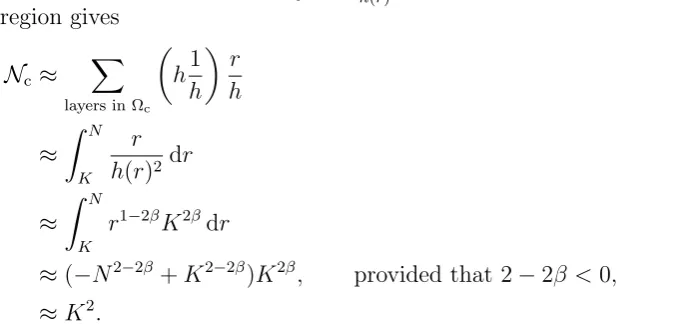
mesh. On each layer with radius r, _Nlayer ≈ _h(r_r). Summing over all layers in the

continuum region gives

Nc ≈ X

layers in Ωc

h1 h

r h

≈ Z N

K

r h(r)2 dr

≈ Z N

K

r1−2βK2β_dr

≈(−N2−2β+K2−2β)K2β_{, provided that 2−2β <0,} ≈K2_.

Therefore, we deduce that the mesh grading should satisfy 1< β < 3

2 to obtain the

optimal cost/accuracy ratio for the error in the energy-norm, K−5/2 _{≈ N}−5/4

h . The

table in_§ 3.3.2 summarises the derivation of this section.

7. Proof of Theorem 3.4

7.1. Existence and error in energy norm. We refer to the inverse function theorem, Theorem 5.1. Let δ_Gh := δEg23 −δf and ¯uh := Πhua. We have already

shown in Theorem 3.2 and Lemma 5.4 that

kGh(¯uh)kU_h∗ ≤η,

hδ_Gh(¯uh)vh, vhi ≥γk∇vhk2L2 for all vh ∈ Uh,

with η=ηint+ηext and

ηint .k∇2_u˜a

kL2_(Ωi₎+k∇3u˜ak_L2_(Ωc₎+k∇2u˜ak2_L4_(Ωc₎

+kh2_∇3_u˜a_k

L2_(Ωc

h)+k∇u˜ a_k

L2₍

R2\BN/2)+N −1

kh2_∇2_u˜a_k

L2_(B

N\BN/2) .Nh−5/4.

For ηext, recall that ∂u(`)f(u) = 0 for all|`| ≥Rf, and that K ≥Rf. We have, on

supp(∂u(`)f(u)), ∇Πhua =∇ua and ∇ϕh =∇ϕ. Thus ηext = 0 and

η=ηint .Nh−5/4.

Using also the Lipscthiz bound from Lemma 5.3 Theorem 5.1 implies, for K

sufficiently large, that there exists a strongly stable minimizerug23_{h ∈ U}h such that

hδEg23

(ug23_h ), ϕhi − hδf(uhg23), ϕhi= 0, ∀ϕh ∈ Uh,

and

k∇ug23_{h − ∇}ΠhuakL2 ≤2η γ .k∇2

˜

uakL2_(Ωi₎+k∇3u˜ak_L2_(Ωc₎+k∇2u˜ak2_L4_(Ωc₎

+_kh2 ∇3_u˜a

kL2_(Ωc₎+k∇u˜ak_L2₍

R2\BN/2)

Adding the best approximation error (6.7) gives

k∇ug23_h − ∇ua_k

L2 ≤ k∇ug23_h − ∇Π_huak_L2 +k∇Π_hua− ∇uak_L2 .Nh−5/4+kh2∇3u˜kL2₍S_Tc

h)+k∇u˜kL2(R2\BN/2) .Nh−5/4.

This completes the proof of Theorem 3.4.

7.2. The energy error. In this section we prove the energy error estimates stated in Theorem 3.4. For the sake of notational simplicity we define Ea

f := Ea−f and Efg23:=Eg23−f.

First, we observe that

|Efg23(u

g23

h )− E

a

f(u

a

)| ≤ |Efg23(u

g23

h )− E

g23

f (Πhua)|+|Efg23(Πhua)− Efa(u

a

)|

=:e1+e2.

The first term can be estimated by (3.6) and the fact that hδEfg23(u

g23

h ), ϕhi= 0 for

allϕh ∈ Uh:

e1 ≤ hδE

g23

f (u

g23

h ),Πhua−ug23h i

+ Z 1 0

(1₋t)_hδ2 Efg23(u

g23

h +t(Πhu

a

−ug23_h ))(Πhua −ug23_h ),(Πhua−ug23_h )idt

.k∇Πhua− ∇uhg23k2L2 .K−5 .N −5/2

h . (7.1)

For the second term we use the fact that_Eg23_{(0) =E}a_{(0), and henceE}g23

f (0) =Efa(0),

to estimate

e2 ≤ |Efg23(0)− Efa(0)|+

Z 1 0

hδEfg23(tΠhua),Πhuaidt−

Z 1

0 hδEa

f(tua), uaidt

≤ Z 1 0

hδEg23

f (tΠhua),Πhuai − hδEfa(tua), vidt

+ Z 1 0 hδEa

f(tua), v−uai dt

=:e21+e22,

wherev : Λ→Rm is an arbitrary test function.

7.2.1. Estimate for e21. To exploit the consistency error estimate we choose v := Π∗

hΠhua defined in (6.4). In this case, similar to estimating ηint, we obtain

e21 . Z 1

0

˜

ηint(t) dtk∇ΠhuakL2₍

R2\Ωah), where

˜

ηint(t) =k∇2_tu˜a_k

L2_(Ωi₎+k∇3tu˜ak_L2_(Ωc₎+k∇2tu˜ak2_L4_(Ωc₎+kh2∇3tu˜akL2_(Ωc h)

+_k∇tu˜a

kL2_(R2_\B

N/2)+N −1

kh2 ∇2_tu˜

kL2_(B

N\BN/2) .tK−5/2_.

From Corollary 3.1 and 6.2 it follows that|∇Πhva(x)|.|x|−2 hence we can deduce

that

e21.K−5/2_K−1

=K−7/2

7.2.2. Estimate for e22. First we observe that by Trapezoidal rule, ifζ _∈C2₍

R) and

ζ(0) =ζ(1) = 0, then we have for someθ _∈[0,1],

Z 1

0

ζ(t) dt=− 1

12ζ

00

(θ).

Letζ(t) := _hδ_Ea

f(tua), v −uai. Then ζ(1) = 0 since δEfa(ua) = 0 and ζ(0) = 0 since

δ_Ea_{(0) = 0 and ∂}

u(`)f(u) = 0 outside defect core while v =ua in the defect core.

Having e22=R1

0 ζ(t) dt we obtain e22.δ3

Ea_(θua_)[ua_{, u}a_{, v} −ua_]

.M3 X

`∈Λ\A

|Dua_{(`)|</sub>2<sub>|Dv(`)−Du}a_(`)|

. Z

R2_\Ωa|∇

˜

ua|2

|∇v− ∇ua|,

where we recall thatv := Π∗

hΠhua. Using the stability (6.5) we obtain

e22 .k∇u˜a_k3

L3_(R2_\Ωa₎+k∇u˜ak2_L4_(R2_\Ωa₎k∇ΠhuakL2₍

R2\Ωa)

. Z ∞

K

rr−6 dr+

Z ∞

K

rr−8 dr

1/2 Z ∞

K

rr−4 dr 1/2

.K−4+K−3K−1 =K−4. (7.3)

Combining (7.1), (7.2) and (7.3) completes the proof of the energy error estimate (3.7) and therefore of our main result, Theorem 3.4.

References

[1] G. Acosta and R. G. Duran. An optimal poincar inequality in l1 for convex domains.Proc. AMS 132(1), 195-202, 2003.

[2] C. Carstensen. Quasi-interpolation and a posteriori error analysis in finite element methods.

M2AN Math. Model. Numer. Anal., 33:1187–1202, 1999.

[3] W. E, J. Lu, and J. Z. Yang. Uniform accuracy of the quasicontinuum method.Phys. Rev. B, 74(21):214115, 2006.

[4] V. Ehrlacher, C. Ortner, and A. V. Shapeev. Analysis of boundary conditions for crystal defect atomistic simulations, 2013.

[5] X. H. Li, C. Ortner, A. Shapeev, and B. Van Koten. Analysis of blended atomistic/continuum hybrid methods.ArXiv e-prints, 1404.4878, 2014.

[6] M. Luskin and C. Ortner. Atomstic-to-continuum coupling. Acta Numerica, 22:397 – 508, 2013.

[7] C. Ortner. The role of the patch test in 2D atomistic-to-continuum coupling methods.ESAIM Math. Model. Numer. Anal., 46, 2012.

[8] C. Ortner and A. Shapeev. Interpolation of lattice functions and applications to atom-istic/continuum multiscale methods. manuscript.

[9] C. Ortner, A. Shapeev, and L. Zhang. (in-)stability and stabilisation of qnl-type atomistic-to-continuum coupling methods, 2014.

[10] C. Ortner and E. S¨uli. A note on linear elliptic systems on _Rd. ArXiv e-prints, 1202.3970, 2012.

[11] C. Ortner and L. Zhang. Atomistic/continuum blending with ghost force correction. ArXiv:1407.0053, to appear in SISC.

[13] Christoph Ortner. A priori and a posteriori analysis of the quasinonlocal quasicontinuum method in 1D.Math. Comp., 80(275):1265–1285, 2011.

[14] C. Schwab. p- and hp- finite element methods: theory and applications in solid and fluid mechanics. Oxford Universiy Press, Oxford, 1998.

[15] T. Shimokawa, J. J. Mortensen, J. Schiotz, and K. W. Jacobsen. Matching conditions in the quasicontinuum method: Removal of the error introduced at the interface between the coarse-grained and fully atomistic region.Phys. Rev. B, 69(21):214104, 2004.

A. Dedner, Mathematics Institute, Zeeman Building, University of Warwick, Coventry CV4 7AL, UK

E-mail address: [email protected]

C. Ortner, Mathematics Institute, Zeeman Building, University of Warwick, Coventry CV4 7AL, UK

E-mail address: [email protected]

H. Wu, Mathematics Institute, Zeeman Building, University of Warwick, Coven-try CV4 7AL, UK