A hydrodynamic limit for chemotaxis in a given heterogeneous environment

warwick.ac.uk/lib-publications

Original citation:

Grosskinsky, Stefan, Marahrens, Daniel and Stevens, Angela. (2016) A hydrodynamic limit for

chemotaxis in a given heterogeneous environment. Vietnam Journal of Mathematics .

Permanent WRAP URL:

http://wrap.warwick.ac.uk/80307

Copyright and reuse:

The Warwick Research Archive Portal (WRAP) makes this work by researchers of the

University of Warwick available open access under the following conditions. Copyright ©

and all moral rights to the version of the paper presented here belong to the individual

author(s) and/or other copyright owners. To the extent reasonable and practicable the

material made available in WRAP has been checked for eligibility before being made

available.

Copies of full items can be used for personal research or study, educational, or not-for profit

purposes without prior permission or charge. Provided that the authors, title and full

bibliographic details are credited, a hyperlink and/or URL is given for the original metadata

page and the content is not changed in any way.

Publisher’s statement:

“The final publication is available at Springer via

http://dx.doi.org/10.1007/s10013-016-0209-8

"

A note on versions:

The version presented here may differ from the published version or, version of record, if

you wish to cite this item you are advised to consult the publisher’s version. Please see the

‘permanent WRAP url’ above for details on accessing the published version and note that

access may require a subscription.

HETEROGENEOUS ENVIRONMENT

IN HONOR OF WILLI J ¨AGER, ON THE OCCASION OF HIS 75TH BIRTHDAY.

STEFAN GROSSKINSKY, DANIEL MARAHRENS, AND ANGELA STEVENS

Abstract. In this paper the first equation within a class of well known chemo-taxis systems is derived as a hydrodynamic limit from a stochastic interacting many particle system on the lattice. The cells are assumed to interact with attractive chemical molecules on a finite number of lattice sites, but they only directly interact among themselves on the same lattice site. The chemical envi-ronment is assumed to be stationary with a slowly varying mean, which results in a non-trivial macroscopic chemotaxis equation for the cells. Methodologi-cally the limiting procedure and its proofs are based on results by Koukkous [20] and Kipnis/Landim [19]. Numerical simulations extend and illustrate the theoretical findings.

Contents

1. Introduction and result 1

2. The general result 5

3. Proof of Theorem 2.1 8

3.1. One block estimate 9

3.2. Two blocks estimate 14

4. Outlook and Examples: numerical simulations 14

5. Concluding remarks 19

References 19

1. Introduction and result

In this paper we derive chemotaxis-like equations as a hydrodynamic limit of a stochastic lattice gas. Chemotaxis describes the directed motion of mainly biolog-ical species towards higher or lower concentrations of chembiolog-ical signals. Here we consider positive chemotaxis of cells, i.e. motion towards higher concentrations of a chemical signal, therefore the chemical signal is denoted aschemo-attractant.

Keller and Segel proposed in [18] a phenomenological chemotaxis model on the macroscopic level for the aggregation and self-organization of the cellular slime mold amoebaDictyostelium discoideum(Dd). This can be written as

∂tρ=∇ · k(ρ, ϑ)∇ρ−χ(ρ, ϑ)∇ϑ

(1.1)

=∇ · k(ρ, ϑ)∇ρ−χ˜(ρ, ϑ)ρ∇ϑ

,

∂tϑ= ∆ϑ+r(ρ, ϑ), (1.2)

Date: March 7, 2016.

Key words and phrases. chemotaxis, interacting stochastic many particle system, hydrody-namic limit, stochastic lattice gas, block estimates.

whereρis the (volume) density of amoebae,ϑis the density of the attractive chem-ical molecules, k and ˜χ =χ/ρ are functional parameters describing the strength of random motion of the cells and their chemotactic sensitivity, respectively, and r comprises the reaction mechanisms. In [18], this cross-diffusion system was mo-tivated by the macroscopic phenomenon being experimentally observed, namely movement of the amoebae in direction of higher concentrations of a chemical sig-nal, i.e. their movement up chemical gradients. Such general types of chemotaxis systems are relevant also in the context of other biological species. One expects this system to be an accurate description for chemotaxis phenomena occuring in systems of many cells and signal molecules. There is a large literature on the formal derivation of macroscopic equations from microscopic particle systems in such set-tings. Rigorously this has been achieved in much fewer cases, e.g. by hydrodynamic or so-called moderate limits. The lack of an ellipticity condition for the limiting PDE-system, respectively the strong clustering of the cells is a major technical problem in this case. In [38] a one-dimensional hyperbolic system is considered, which can describe a kind of negative chemotaxis behavior, but here we deal with positive chemotaxis and aggregation.

The first rigorous derivation of a general class of chemotaxis systems from a sto-chastic interacting many particle system was given in [37], where the cells and the chemical molecules interact moderately with each other in the sense described in [28]. The motion of the cells and the molecules are governed by interacting sto-chastic differential equations, and production and decay of the chemical molecules are modeled via Poisson point processes. In [37] explicit error estimates could be given, which show that the total number of particles does not have to be too large for the limiting PDE-system to be a good approximation for the particle model. The moderate rescaling requires that in the limiting procedure, when the total particle number (cells and chemical molecules) tends to infinity, the main range of inter-action of the particles tends to zero. The number of particles sensed in this main range of interaction tends to infinity too, while this number is still only a vanishing fraction of the total particle number. This is sufficient for correlations to become small enough in the limit. The main technical complication in the proof is the cross-diffusion structure of the chemotaxis system. The ellipticiy condition, heavily used in [28], is no longer valid in this case. To overcome this problem, two shadow systems were introdcued, in order to freeze the critical non-linearity and a priori es-timates were derived. This technique applies also to more general systems of PDEs.

In principle it would be desirable to also derive chemotaxis like systems as hydro-dynamic limits in the sense of [19]. In this paper, we rigorously derive equation (1.1) from a microscopic stochastic many particle system on a lattice, so only one equation, not the full system. The cells are assumed to interact via a finite number of lattice sites with the chemical molecules. This corresponds to the assumption that the cells detect chemical molecules in a fixed small region around themselves. They do not change the chemical environment in this case. The interaction of the cells among themselves takes place only at the same lattice site and not among cells located on neighboring sites. This interaction is described by a function g which among others fulfills conditions comparable to an ellipticity condition for the related limiting PDE. These will be specified later. So we consider the case, where a too strong clustering/aggregation of cells - a typical and important effect of chemotaxis and self-organization in Dd - is avoided.

[27, Introduction]. To be more precise, we are modeling the cells/particles by an interacting particle system as introduced in [34] and derive limit equations via a hydrodynamic limit, analogous to the procedure in [19]. Interacting particle sys-tems in this sense are continuous-time Markov jump processes which also involve discrete particles moving on a lattice.

So far we were not able to derive the full system (1.1), (1.2) as hydrodynamic limit. It seems to be a major challenge to identify suitable particle models with invariant product measures. This would be one option in order to prove a hydrodynamic limit for systems of equations such as (1.1) and (1.2). Hydrodynamic limits without product measures for single-species monotone particle systems where established in [4, 5]. Stochastically monotone systems preserve a partial order on state space over time, which allows the use of coupling techniques following first results in [32]. Monotonicity usually leads to homogeneous mass distributions, and indeed it has been shown recently that particle systems with invariant product measures that exhibit a particular form of clustering are necessarily non-monotone [31].

A generic example which exhibits invariant product measures is given by the zero-range process (ZRP), where the jump rate of particles at any given site depends only on the occupation number at this site. It is known, see [14], that multi-species ZRPs have invariant product measures if the jump rates of particles satisfy certain symmetry relations, i.e. the Onsager relations. However, in our case this would not allow purely diffusive motion of the chemo-attractant in (1.2). Instead, the attractive chemical molecules would need to undergo a kind of chemotactic motion too, in order for the Onsager relations to hold. From the modeling point of view this is definitely not the case here.

Another method to derive a system of a PDE coupled to an ODE via a hydrody-namic limit without the use of invariant product measures was introduced in [10] for a specific two-species cellular system on the lattice. The authors new method employs energy estimates for the mesoscopic empirical averages of the particles oc-cupation number by which they obtain H2

1 a-priori bounds and thus are able to

derive a substitute for the two block estimates. For the most crucial terms in their setting homogenization techniques are used, which play the role of the one block estimates. For a discussion of the respective particle model itself see also [25]. It would be interesting to see whether in our case one can find scaling regimes where the existence of gradients (and not only densities as in [10]) can rigorously be proved for the full limiting PDE system.

One typical approximation of system (1.1), (1.2) is to assume a quasisteady chemo-attractant density, i.e. to set the left hand side of (1.2) equal to zero. Formally, this is justified by assuming that the diffusivity of the chemo-attractant is much larger than the random motion of the cells, see e.g. [16]. There are also recent results on random walks in dynamic random environments driven by exclusion processes [3], which are based on separation of time-scales argument. Otherwise there are only very few rigorous results on hydrodynamic limits for two-species systems, see e.g. [12, 7], since such processes are in general also non-monotone.

It is obvious from a modeling point of view, how a full chemotaxis model for the behavior of particles on a lattice could look like, compare e.g. [29]. One ansatz relates to attractive reinforced random walks for many particles with diffusion and decay of the attractive weight. Deriving a hydrodynamic limit for such, or similar models would be the final goal. We expect the Keller-Segel model to also hold in this context, but a proof is still missing.

order to obtain a non-trivial macroscopic chemotactic motion, we impose a slowly varying mean on the random chemical environment. There have been several stud-ies of hydrodynamic limits of particles in random media: The hydrodynamic limit for a ZRP a with stationary, ergodic environment on the sites has been obtained in [20], and corresponding large deviations have been considered in [21]. The case of a stationary, ergodic environment on the edges was treated in [13]. The hydrody-namic limit for the ZRP with slowly varying but not random environment is given in [9]. For a result unifying all these situations of “locally convergent” media in the special case of the simple exclusion processes compare [17]. Our main result in the present paper concerns the modeling of chemotaxis via a ZRP in a random envi-ronment with slowly varying mean and it is summarized in Theorem 2.1, Section 2. A special case of this result is given in Corollary 1.1 below.

At each site x ∈ _Td

N on the periodic lattice T d

N = {1, . . . , N}

d _{one distributes}

ζ(x) ∈ _N molecules of the chemo-attractor such that ζ(x) is a Poisson random variable with parameterϑ(_Nx) and these are kept fixed for all time. Letf :_N→[a, b] for some a, b >0 and set

e

f ϑ(_Nx):=

E

1 f(ζ(x))

−1

.

Now we specify the type of chemotactic motion we consider here for the cells. We start with an initial distribution of η(x) cells at x∈ _Td

N. All cells perform inde-pendent random walks with a site-deinde-pendent jump-rate which isN2_{f(ζ(x)). Thus}

each cell remains at its current sitex∈_Td

N for an exponentially distributed random waiting time with parameter N2_{f(ζ(x)) and then jumps to a random neighboring}

site on the lattice. In this way, particles are more likely to stay at a sitexiff(ζ(x)) is large and thereforef is one way of formulating the microscopic behavior which results in a chemotactic drift towards higher concentrations of the chemical signal. To take the limit asN → ∞, we embed the discrete torusTdN into the continuous torus _Td ₌

Rd/Zd viax7→ Nx. Thus the number of cells in an intervalI ⊆T d _is

given by

#{cells inI}= X

x∈N I∩TdN

η(x),

where N I isI rescaled byN. The cell density inI is then obtained as

P

x∈N Iη(x)/(|I|Nd).

Corollary 1.1. Let the cells initially be distributed with a profile ρ0(u), i.e. for each interval I⊆_Td_{, the density converges in probability:}

lim N→∞

#{cells inI at time0}

|I|Nd =

1 |I|

Z

I

ρ0(u)du.

Then for all later times t >0 and all intervals I, almost surely with respect to the distribution of chemical molecules ζ, it holds that

lim N→∞

#{cells inI at timet}

|I|Nd =

1 |I|

Z

I

ρt(u)du

in probability, where ρt solves

(1.3) ∂tρt(u) = ∆

e

f(ϑ(u))ρt(u)=∇ ·hfe(ϑ(u))∇ρt(u) +fe0(ϑ(u))ρt(u)∇ϑ(u) i

,

which is of the form (1.1).

Remark 1.2. (1) The assumption of independent random walks treated in Corol-lary 1.1 yields a linear limit equation and is much weaker than necessary, see The-orem 2.1. It is presented here in order to give the reader an intuition for the connection between the macroscopic bias fe(ϑ(u)) induced by the chemical signal

and the related microscopic bias f(ζ(x)).

(2) Note that instead of the Poisson distribution, we can let the environment be given by any distribution inNdepending continuously (in distributional topology)

on its parameter.

(3) In case of a stationary chemical environment, the solution is always global and no blow-up can occur, thus excluding a prominent feature of the full chemotaxis system, where the possibility of finite time blow-up in two space dimensions for a suitable parameter range is of important biological relevance for self-organization phenomena in the cellular slime mold amoebae Dd, [8], [16].

(4) Finally, let us mention that some microscopic descriptions for chemotactic cell motion are based on the feature that the cells can detect concentration gradients along their cell surface. Our result supports the idea that chemotactic effects can also occur if the cells only sense the absolute values of the concentration of the chemo-attractant without needing to sense its (local) gradients. An alternative ap-proach would be to let each particle perform asymmetric random walks (and its nonlinear versions involving a zero range interactiong(·), see below) with jump rates across edges of the lattice proportional to p(x, y). Herex,y are neighboring sites, andp(x, y) is a random variable, which in our case is determined by the attractive chemical environment ζ(x), see also [29] and the microscopic approaches in [2]. A typical example for an asymmetric random walk would bep(x, y) =f ζ(y)−ζ(x)

, representing a microscopic gradient for an appropriate function f. This approach would lead us to consider problems of the type investigated in [13].

(5) For positive chemotaxis effects, i.e. clustering/aggregation of the cells the sign of the second term on the right hand side of (1.1), (1.3) is crucial. Further, already in [33] it was pointed out that the diffusivity ˜f,k and the chemotactic sensitivity −f˜0, ˜χof the cells are not completely independent functionals. A suggestion in [33] is that the diffusivity ˜f in (1.3) relates to the chemotactic sensitivity−f˜0, which is supposed to have a positive sign in case of positive chemotaxis, as follows:

˜

f0 =−χ0f˜Φ˜0(ϑ) for a suitable function ˜Φ, e.g. ˜Φ(ϑ) =ϑandχ0>0.

This results in ˜f =Cexp(−χ0Φ(˜ ϑ)), e.g. ˜f =Cexp(−χ0ϑ).

So for large chemical concentrations ˜f becomes small.

The outline of the paper is as follows. In Section 2, we present a general result on hydrodynamic limits in a random environment with slowly varying mean. Its proof is given in Section 3 where we highlight the differences to the proofs found in [20, 19]. Then in Section 4, we show how to deduce Corollary 1.1 from the general result and present numerical simulations of the particle system.

2. _{The general result}

In this paper, we apply theentropy methodas given in [15] to obtain a generalization of equation (1.3), namely for the chemotactically moving cells, in a stationary, yet random, environment, which represents the density of a heterogeneously distributed attractive chemical signal. To avoid technicalities concerning boundary conditions, we shall work in a periodic domain. Thus we consider a Markov (Feller) process, describing the motion of the cells, with state spaceNT

d

N, where_Td

elements of _Td

N will be denoted by the letters x, y, z and are called microscopic variables. Two microscopic sites x, y∈TdN are calledneighbors, in shortx∼y, if |x−y|= 1. The discrete torus is embedded in the continuous torus Td =Rd/Zd

viax7→x/N. Elements of the continuous torus will be denoted byuand are called

macroscopicvariables. For simplicity, we consider only symmetric nearest-neighbor jumps; then the Markov process is given by the generator

(2.1) LNf(η) =

X

x∼y

g(η(x))pN_x f(ηx,y)−f(η)

for all f ∈Cb(NT

d

N), where the sum is taken over all (ordered) pairs of neighbors

x and y. Here ηx,y _{denotes the configuration obtained from η after one particle} has jumped from site x to y and pN

x > 0 describes the chemical environment. Throughout this article, we assume that

pN_x =v(_Nx) +qx,

where v ∈ C1(Td,R+) describes the slowly varying mean of the environment and

(qx)_x∈Zd⊂_RZ d

is a uniformly boundedstationary andergodicsequence of random variables with zero mean. In order to avoid degeneracies, we assume strictly positive jump rates, i.e. without loss of generality we assume that v andq are chosen such that pN

x ∈ [a, b] with 0 < a < b. We denote the law of q by m, so that m is a probability measure on _RZd_.

It is also possible to think of pN

x as a random variable. Note, however, that for technical reasons in what follows we fix the ergodic part q of the environment independently of N. The dependence of the jump rates on the number of cells is given by the function g:N→[0,∞). In addition to the standard condition

g(n) = 0 ⇔n= 0

to avoid degeneracies, we make the following regularity assumptions on g through-out the paper.

Assumption 1. (i) Suppose that g is uniformly Lipschitz-continuous, i.e. there exists a constant g∗ such that

sup n∈N

|g(n+ 1)−g(n)| ≤g∗.

(ii) Further assume that g grows at least linearly, i.e. there existsg0>0 such that

inf n∈N+

g(n) n ≥g0.

These assumptions are not optimal but they are standard in the literature, see e.g. [19, Theorem 5.1.1], on which our proof is based. Under these assumptions, the process with generator (2.1) has invariant product measures νN,p _{that satisfy the}

detailed balance condition

pN_xg(n)νN,p[η(x) =n]νN,p[η(y) =k]

=pN_yg(k+ 1)νN,p[η(x) =n−1]νN,p[η(y) =k+ 1]

for all neighborsx, y∈TdN andk, n∈N.

Indeed for anyϕ≥0, there exists such a measureνN,p

ϕ given by

(2.2) ν_ϕN,p(η) = Y

x∈TdN

(pN x)−1ϕ

η(x)

Z((pN

where g(n)! =g(1)g(2). . . g(n),g(0)! = 1 and

(2.3) Z(ϕ) =

∞

X

n=0

ϕn g(n)!

is the partition function. The detailed balance condition ensures that the generator LN in (2.1) isL2(νϕN,p)-selfadjoint and in particular the measureνϕN,pis an invariant product measure. Letν1

ϕdenote the one-site marginal without environment, i.e.

ν_ϕ1(n) = ϕ n

Z(ϕ)g(n)! .

The associated density then is

(2.4) M(ϕ) =_Eν1

ϕ[η(0)].

Assumption 1 implies that Z is finite on [0,∞). Hence the product measureνN,p ϕ exists for allϕ∈[0,∞) and environments (pN

x)x∈TdN. The parameterϕ≥0 is called

fugacity, and it controls the expected particle density which is given by

(2.5) R(u, ϕ) :=_Em

h

M_v(uϕ_)+q

0

i

for all u∈Td. The family of distributions (2.2) is also called the grand-canonical

ensemble. One can show that for each u ∈ Td, the function R(u,·) is strictly

increasing, cf. [19], and we then define Φ(u,·) to be its inverse function. Note that

Em

h EνN,p_Φ(x

N,ρ)

η(0)i

=ρ and _Em

h EνϕN,p

g(η(x))pN_xi

=ϕ.

We shall see that the limit equation is given by

(2.6) ∂tρt(u) = ∆Φ(u, ρt(u)).

Finally we need a suitable notion of distance between probability measures, which in our case is given by the relative entropy. Consider measuresν, µ∈P(_NTdN) such

that µis absolutely continuous with respect to ν (i.e. µ ν). Then the relative entropy is given by

H(µ|ν) =

Z

NT

d N

logdµ

dν(η)dµ(η),

where dµ_dν denotes the Radon-Nikodym derivative ofµwith respect toν. The main result of this section is the following.

Theorem 2.1. Let µN

0 ∈P(NT

d

N)be the initial datum of the particle process with

an associated initial profile ρ0∈L∞(Td), i.e. it holds

lim N→∞µ

N 0 1 Nd X

x∈TdN

G(_Nx)η(x)−

Z

Td

G(u)ρ0(u)du ≥δ

= 0 m-almost surely

for all G∈C(Td)andδ >0. Furthermore we suppose the bounds

H(µN0|ν

N,p ϕ )≤CN

d

and EµN 0

X

x∈TdN

η(x)2

≤CNd

to hold for some (and hence all) ϕ > 0. Denote by µN

t ∈ P(NT

d

N) the measure

obtained from the evolution of the ZRP with rate function g and byρt ∈L∞(Td) the density obtained from equation (2.6). Then under Assumption 1, it holds that

lim N→∞µ

N t 1 Nd X

x∈TdN

G(_Nx)η(x)−

Z

Td

G(u)ρt(u)du

≥δ

= 0 m-almost surely

Remark 2.2. In order to fully connect Corollary 1.1 with Theorem 2.1, we note that weak convergence of the empirical measures implies convergence of the densities over intervals by the Portmanteau theorem [6, Theorem 2.1]. This follows from the absolute continuity (with respect to the Lebesgue measure) of the limit measure ρt(u)du.

To prove this result, we adapt the method in [20] to a random environment with slowly varying mean. The paper [20] is based on the entropy method given in [15] and proves a hydrodynamic limit for a zero range process in a stationary (ergodic) random environment. The case of a zero range process in a slowly varying deter-ministic environment was treated in [9]. Thus, from a purely technical point of view, our result is a combination of the previous two. Indeed, our method is close to the methods presented in [20]. Therefore we mainly highlight the differences here. The basic idea of the proof lies in the fact that the slowly varying mean is locally almost constant and hence in small boxes we are essentially in the situation of [20].

3. _{Proof of Theorem 2.1}

The first step of the proof is to obtain a priori bounds and tightness of the particle process. Indeed we can understand the convergence result of Theorem 2.1 in terms of the empirical measure

αN_η (du) = 1 Nd

X

x∈TdN

η(x)δx

N(du)∈ M+,

whereδu denotes a Dirac delta,u∈Td, andM+ is the space of all positive Radon

measures onTd. For allt≥0, the configurationηtis a random variable distributed according to µN

t . Note that it suffices to prove Theorem 2.1 for all 0 ≤ t ≤ T with a fixed, but arbitrary, T > 0. Since for any environment p the ZRP is a jump process on the state space, (ηt)t∈[0,T] is a random variable on the path space

D([0, T];NT

d

). Here D([0, T];NT

d

) denotes the space of functions [0, T] → NT

d

that are right-continuous in time with left limits. We denote the distribution of (ηt)t∈[0,T] byµN. In the same vein, (αηNt)t∈[0,T] is a random variable on the path

space D([0, T];M+); letQN,p denote its distribution. The entropy dissipation of

µN

t can be defined in terms of the Dirichlet form

D(µN_t |νN,p ϕ ) :=

Z

NT

d N

s

dµN t dνϕN,p

LN

s

dµN t dνϕN,p

dν_ϕN,p.

Throughout this paper we suppose that the assumptions of Theorem 2.1 are satis-fied.

Lemma 3.1. It holds that

H(µN_t |νϕN,p)≤CN

d _{for allt}

∈[0, T] and 1

T

Z T

0

D(µN_t |νϕN,p)dt≤CN d_.

Lemma 3.2. For any environmentp, the sequence of probability measures(QN,p_)N∈

N

is tight.

Lemma 3.3. For any environmentp, all limit pointsQ∗,p of (QN,p_)N

∈N are

sup-ported on {π ∈ D([0, T];M+(Td)) : πt(du) du}, i.e. at each time t, the limit measures are absolutely-continuous with respect to the Lebesgue measure.

The proofs of Lemma 3.1 – 3.4 are similar to the proofs of the corresponding results for the usual ZRP, see Lemma 2.1 – 2.4 in [20] and Lemma V.1.5 and V.1.6 in [19]. Once these results have been obtained, Theorem 2.1 is a straight-forward consequence. The main difficulty consists in the proof of the so-called replacement lemma, which is the key to Lemma 3.4. In order to state the replacement lemma, we need some additional notation to describe averages over mesoscopic blocks. Set

ηl(x) = 1 (2l+ 1)d

X

|x−y|≤l η(y)

and

V_x,lp (η) :=

1 (2l+ 1)d

X

|x−y|≤l

pN_yg(η(y))−Φ(_Nx, ηl(x))

.

Lemma 3.5 (Replacement Lemma). For every δ > 0, m-almost surely it holds that lim sup →0 lim sup N→∞ µN Z T 0 1 Nd X

x∈TdN

V_x,Np (ηt)dt≥δ

= 0.

In the remainder of this section we will mainly prove Lemma 3.5, where we sketch the modifications necessary to adapt the proof in [20] in order to take into account the slowly varying average of the environmentv(_Nx). First we prove the replacement over small boxes of sizel∈N.

3.1. One block estimate.

Lemma 3.6 (One Block Estimate). It holds that

lim sup l→∞

lim sup N→∞ Eµ

N Z T 0 1 Nd X

x∈TdN

V_x,lp (ηt)dt

= 0

m-almost surely.

Setting

f_tN(η) = dµ N t dνϕN,p

(η), FN(η) =

Z T

0

f_tN(η)dt,

we see that

EµN

Z T

0

1 Nd

X

x∈TdN

V_x,lp(ηt)dt

= 1 Nd

X

x∈TdN

Z

NT

d N

V_x,lp(η)FN(η)dν_ϕN,p(η).

Lemma 3.1, together with convexity of the entropy and Dirichlet form, yields the bounds

HN,p(FN) :=H(FN dν_ϕN,p|dν_ϕN,p)≤CNd,

DN,p_(FN_{) :=D(F}N _dνN,p ϕ |dν

N,p ϕ )≤CN

d−2_.

(3.1)

For future reference, we also note the following expression of the Dirichlet form via the density FN_{. It holds that}

(3.2) DN,p_(FN_{) =}X

x∼y Z NT d N 1 2p N xg(η(x))

q

FN_(ηx,y₎₋q_FN_(η)2

dν_ϕN,p.

Lemma 3.7. Under the conditions of Theorem 2.1, we have

lim sup A→∞

lim sup l→∞

lim sup N→∞

sup p,f

Z

NT

d N

1 Nd

X

x∈TdN

V_x,lp (η)χ{ηl_(x)>A}(η)f(η)dν_ϕN,p(η) = 0.

where the supremum is taken over all densities f such that HN,p_(FN_{) ≤ CN}d_, DN,p_(FN_)≤CNd−2 _{and all environments p=p}N _{⊂[a, b]}TdN_{. For every set} A_{, we}

denote by χA the characteristic function ofA.

Therefore we just need to prove

lim sup l→∞

lim sup N→∞

1 Nd

X

x∈NT

d N

Z

NT

d N

V_x,l,Ap (η)FN(η)dν_ϕN,p(η) = 0

m-almost surely, where we setV_x,l,Ap (η) :=V_x,lp(η)χ{ηl_(x)≤A}(η). In fact, due to the

bounds (3.1) on the Dirichlet form of FN_{, it suffices to find an upper bound for}

(3.3) 1 Nd

X

x∈TdN

Z

NT

d N

V_x,l,Ap (η)FN(η)dν_ϕN,p(η)−γCN2−dDN,p_(FN₎

for all γ > 0. Next we restrict the problem to translations Λx,l of the small box Λl:={−2l, . . . ,2l}d. Denote byνϕx,l,p the Λx,l-marginal ofνϕN,pand byFx,l(η) the density of the Λx,l-marginal of the measureFN(η)dνϕN,p(η) with respect toνϕx,l,p. We will sometimes drop the index for x= 0 for such quantities when taken at the origin. Furthermore we define a Dirichlet form on Λx,l by

D_x,lp (f) = X

y∼z

y,z∈Λx,l

I_y,zp (f), where we have set

I_y,zp (f) =1 2

Z

NTdN

pN_yg(η(y))pf(ηy,z₎₋p

f(η)

2

dν_ϕN,p.

By convexity of the ”bond”-Dirichlet forms Ip

y,z, we haveIy,zp (Fx,l)≤Iy,zp (FN) for all neighbors y, z∈Λx,l and thus

1 Nd

X

x∈TdN

Dp_x,l(Fx,l)≤C(l) Nd D

N,p_(FN_).

Hence instead of expression (3.3), we just need to find an upper bound for

(3.4) 1 Nd

X

x∈TdN

Z

NTdN

V_x,l,Ap (η)Fx,l(η)dνx,l,pϕ (η)−γC(l)N

2

Dp_x,l(Fx,l)

.

Next we need to take care of the random part of the environment. The method to keep track of the environment is due to [20] and constitutes the main deviation from the proof of the hydrodynamic limit for the usual ZRP as exhibited in [19]. Thus we fixα, δ >0 and letn∈Nbe sufficiently large such that n1 < δ. Divide the interval [a, b] into sub-intervals of length not greater thanδ(b−a) viaIδ

j = [βj, βj+1)

for 0≤j≤n−2 where

βj =a+ (b−a) j

n (j= 0, . . . , n−1)

and Iδ

n−1= [βn−1, b]. Fixk < land letL= [(2l+ 1)/(2k+ 1)]d, where [x] denotes

the Gaussian bracket, i.e. the largest integer smaller than or equal tox∈_R. Now we divide Λlinto disjoint cubes of the formx+ Λk, where we takeBi,i= 1, . . . , L−1, such that

Then set BL = Λl\S L−1

i=1 Bi and without restriction takex1 = 0, i.e.B1 = Λk. Also set Bi(x) =x+Bi forx∈Zd. Forx∈TdN,α∈(0,1) and q∈[a, b]Λl, set

(3.5)

N_x,j,il,k,δ(q) := 1 (2k+ 1)d

X

z∈Bi(x)

χIδ j(qz),

Al,k,δ_x,i,α:=n(qz)z∈Λl:

N

l,k,δ

x,j,i(q)−Em[χIδ j(qz)]

≤α, j = 0, . . . , n−1 o

,

Al,k,δ_x,α :=

(

(qz)z∈Λl:

1 L

L

X

i=1

χ_Al,k,δ x,i,α

(q)≥1−α

)

.

SinceV_l,Ap ≤C(A) is bounded, the expression (3.4) is bounded form above by

(3.6)

1 Nd

X

x∈TdN

(

χ_Al,k,δ x,α (p)

Z

NT

d N

V_x,l,Ap (η)Fx,l(η)dν_ϕx,l,p(η)−γC(l)N2D_x,lp (Fx,l)

+C(A)(1−χ_Al,k,δ x,α (q))

)

.

Now we take care of the non-random part of the enviroment. To this end, set

e

Al,k,δ_x,u,α=n(pz)z∈Λl :pz=qz+vz, q∈A

l,k,δ x,α ,sup

z∈Λl

|vx+z−v(u)| ≤α

o

Since vis smooth, in particular (uniformly) continuous, for everyαwe can choose N large enough such that vx+z :=v((x+z)/N) does not differ from v(x/N) by more than α. Thus (3.6) is bounded from above by

(3.7)

1 Nd

X

x∈TdN

(

χ e

Al,k,δ

x, x_N,α

(p)

Z

NT

d N

V_x,l,Ap (η)Fx,l(η)dν_ϕx,l,p(η)−γC(l)N2Dp_x,l(Fx,l)

+C(A)(1−χ_Al,k,δ x,α (q))

)

.

Since the random partqof the environment is stationary and ergodic by assumption, it holds

1 Nd

X

x∈TdN

1−χ_Al,k,δ x,α (q)

_N→∞

−−−−→Pm(q /∈Al,k,δ0,α ),

which in turn vanishes by ergodicity in the limit as l → ∞ and k → ∞. The remaining term in (3.7) is bounded from above by

sup u∈Td

χ e

Al,k,δ_[uN],u,α(p)

Z

NT

d N

V_[p_uN],l,A(η)F[uN],l(η)dνϕ[uN],l,p(η)

−γC(l)N2Dp_[uN],l(F[uN],l)

.

Again τ−[uN]p is in Ae

l,k,δ

0,u,α for large enough N and the term involving Φ(

[uN]

N , ρ) which appears inV_[p_uN],l,Aconverges uniformly inuandρ≤Ato Φ(u, ρ). Thus we see that, up to an error that vanishes as N → ∞, it suffices to estimate

(3.8) sup u∈Td

sup p∈Ael,k,δ_0,u,α

sup f

Z

NΛl

V_l,Ap (η)f(η)dν_ϕl,p(η)−γC(l)N2D₀p_,l(f)

where the inner supremum is taken over all densitiesf on_NΛl_{. For fixedl}∈

N, the

termV₀p_,l,Ais only non-zero on the compact space of configurations in_NΛl_{of at most}

(2l+ 1)d_{A particles, the Dirichlet form is lower-semicontinuous and this property} is conserved by the supremum. Hence the limit superior of (3.8) is bounded from above by

(3.9) sup

u∈Td

sup p∈Ael,k,δ_0,u,α

sup f

Z

NΛl

V_l,Ap (η)f(η)dν_ϕl,p(η),

where now the inner supremum is taken over all densitiesf on_NΛl _{with vanishing}

Dirichlet formDp_l(f) = 0. A densityf has vanishing Dirichlet form if and only if it is constant along all hyperplanes of a given number of particles. With this in mind, we introduce the canonical measures

ν_l,Kp (·) :=ν_ϕ0,l,p(· |P

x∈Λlη(x) =K).

Since the probability density f is constant on {P

x∈Λlη(x) = K}, we can

esti-mate (3.9) from above by

(3.10) sup u∈TdN

sup p∈Ael,k,δ_0,u,α

max

0≤K≤(2l+1)d_A

( Z NT d N 1 L L X i=1 Z 1 (2k+ 1)d

X

x∈Bi

pxg(η(x))

−Φ u, K

(2l+1)d

dν

p l,K(η)

)

,

where we have inserted the explicit form ofV₀p_,l,Aand applied the triangle inequality.

For givenuandp∈Ae

l,k,δ

0,u,α, we defineϕ p K by

(3.11) Eνl,p

ϕp_K

[ηl(x)] = K (2l+ 1)d.

Note that 0≤ϕp_K ≤C(A) is uniformly bounded in 0≤K≤(2l+ 1)d_{A andl∈}

N.

The next lemma concerns the closeness of the grand-canonical and the canonical measures.

Lemma 3.8 (Equivalence of ensembles). For all F :_NΛk _→

Rwith finite second moments with respect toνk,p

ϕ for allϕ≤C(A), it holds that

lim l→∞ sup

p∈[a,b]Zd

max

0≤K≤(2l+1)d_A

Eν

l,p ϕp_K

F(η)−Eν_l,Kp

F(η)

= 0.

Proof. Thanks to the uniform boundsa≤px≤b, the equivalence of ensembles can be proved as explained in [19, Appendix 2], see also [20, Lemma 3.3].

By applying Lemma 3.8 to

F(η) = 1 (2k+ 1)d

X

x∈Bi

pxg(η(x)),

we just need to find an upper bound for

(3.12) sup u∈TdN

sup p∈Ael,k,δ_0,u,α

max

0≤K≤(2l+1)d_A

( Z NT d N 1 L L X i=1 Z 1 (2k+ 1)d

X

x∈Bi

pxg(η(x))

−Φ u,_(2l+1)K d

dν

l,p ϕp_K(η)

)

The next two lemmas yield convergence of this expression in the limit as l → ∞ and then k→ ∞. In a certain sense, the first lemma describes the “ergodic” error between spatial averages and the quenched grand-canonical average.

Lemma 3.9. For allα, δ >0, it holds that

lim sup k→∞

lim sup l→∞

sup u∈TdN

sup p∈Ael,k,δ_0,u,α

max

0≤K≤(2l+1)d_A

( Z

NTdN

1 L L X i=1 Z 1 (2k+ 1)d

X

x∈Bi

pxg(η(x))−ϕpK

dν

l,p ϕp_K(η)

)

= 0.

The second lemma describes the difference between the quenched and annealed grand-canonical averages.

Lemma 3.10. It holds that

lim sup δ→0 lim sup α→0 lim sup k→∞ lim sup l→∞ sup u∈TdN

sup p∈Ael,k,δ_0,u,α

max

0≤K≤(2l+1)d_A

ϕ

p

K−Φ u, K

(2l+1)d

= 0.

Proof of Lemma 3.9. Under the lawν_ϕl,pp K

, the random variables (pxg(η(x))−ϕ p K)x∈Bi

are independent with zero mean. Furthermore their variance is uniformly bounded by continuity in pandK. Thus the expression to be bounded vanishes by a law of

large numbers.

Proof of Lemma 3.10. The absolute value in the given equation is obviously con-tinuous inpand K. Using the fact thatAe

l,k,δ

0,u,α is closed andv(·) is continuous, it is straight-forward to prove that the supremum over pand K is continuous with respect tou. Hence for everyl∈N, the supremum in the hypothesis is achieved for

some u∈_Td_{, p∈}

e

Al,k,δ_0,u,α and 0≤K ≤(2l+ 1)d_{A. For these maximizers, let ϕbe} a limit point asl→ ∞andϕp_K the corresponding subsequence. Then the absolute value in the given formula in Lemma 3.10 is bounded from above by

(3.13) ϕ

p K−ϕ

+

ϕ−Φ

u,_(2l+1)1 d

P

z∈ΛlM

ϕ pz + Φ

u,_(2l+1)1 d

P

z∈ΛlM

ϕ pz

−Φu,_(2l+1)1 d

P

z∈ΛlM

ϕp_K pz

,

where we have used (2.4), (2.2) and (3.11). By continuity and since ϕp_K converges to ϕas l→ ∞, the first and last terms vanish in the limit. Now by definition of Φ and (2.5), we write

ϕ= Φ(u, R(u, ϕ)) = Φu,Em

h

M _v(uϕ_)+q

0

i

.

Since Φ(u,·) is Lipschitz continuous uniformly inu∈_Td_{, the second term in (3.13)} is bounded from above by a multiple of

E m h

M _v(uϕ_)+q

0

i

− 1

(2l+ 1)d

X

z∈Λl

M _pϕ

z .

By the triangle inequality, since p ∈ Ae

l,k,δ

0,u,α is of the form pz = qz +vz with |vz−v(u)| ≤ α, and since M is Lipschitz continuous, this term is bounded from above by 1 L L X i=1

χ_Al,k,δ 0,i,α

(q)

E m h

M _v(uϕ_)+q

0

i

− 1

(2k+ 1)d

X

z∈Bi

M _v(uϕ_)+q

for all small enough α >0. Hence it is enough to consider

sup q∈Al,k,δ0,1,α

Em

h

M _v(uϕ_)+q

0

i

− 1

(2k+ 1)d

X

z∈Λk

M _v(uϕ_)+q

z .

For each q, the absolute value in this formula is bounded from above by

E m h

M _v(uϕ_)+q

0 i − n−1 X j=1

M _v(uϕ_)+β

j

m(I_jδ)

+ n−1 X j=1

M _v(uϕ_)+β

j

m(I_jδ)−N_j,l,k,δ₁ (q) + 1 (2k+ 1)d

X

z∈Λk

n−1 X

j=0

M _v(uϕ_)+β

j

−M _v(uϕ_)+q

z

χ_Iδ j(qz)

.

By the Lipschitz-continuity of M and sincen≤Cδ−1_{, this expression is bounded}

from above byC(δ+αδ−1_{) for allq∈A}l,k,δ

0,1,α. Taking the limit, first forα→0 and then forδ→0, finishes the proof of the one block estimate.

Remark 3.11. The above estimates correspond to the approximation of the inte-gral with respect to the measure mby an integral of simple functions.

3.2. Two blocks estimate. Similarly, we can prove the two blocks estimate, which shows that the difference between averages over boxes of sizelandN is negligible in the limit.

Lemma 3.12 (Two Blocks Estimate). It holds that

lim sup l→∞ lim sup →0 lim sup N→∞ sup |y|≤N

EµN

Z T

0

1 Nd

X

x∈TdN

η_tl(x+y)−η_tN(x) dt

= 0

m-almost surely.

We will skip the proof here and just note that it follows in a similar manner like the one block estimate — the main difference lying in restricting the process to two boxes of size l (that are at most N apart) instead of just one. For details, the reader may refer to [19, 20].

4. _{Outlook and Examples: numerical simulations}

In this section, we present examples for chemotactic motion of particles in a slowly varying chemical attractive environment in a slightly more general setting than our theory has so far addressed. This is done in order to get further insight into the behavior of such particle systems. Consider the (smooth) functionϑ:Td →(0,∞).

Assume that the attractive chemical environment ζ(x) on the lattice TdN is given by independent Poisson random variables with parameterϑ(_Nx) at sitex∈_Td

N. As before, letmdenote the law of this random environment. One might think of this distribution as resulting from independent diffusion of attractive chemical molecules on a time-scale much faster than the typical time-scale of the diffusive motion of cells so that it is effectively time independent with respect to the random motion of the cells. This assumption on the time-scales is biologically reasonable and helpful also for theoretical reasons as outlined in the introduction. We suppose that the cells motion is described by a Markov process with generator given by (2.1), where the environmentpN depends on the number of attractive chemical moleculesζ via

Thus f : _N → (0,∞) provides a microscopic description of the chemical bias. For simplicity, let us suppose for the rate g(η) = η, i.e. that the cells diffuse independently in the random environment pN_{. Note that the “random part”} pN

x −Em[f(ζ(x))] consists of independent but not stationary random variables, so our theory given before does not apply directly in this case. However, on local boxes the density ϑ(_Nx) is approximately constant, say ϑ(u), and the environment consists of almost identically and independently distributed particles, so that we expect that with techniques as given above a hydrodynamic limit can be derived in this case, too. To identify this limit, consider M given as in (2.4). Since g is the identity,νϕ1 is a product of identical Poisson distributions with parameterϕand it follows M(ϕ) =ϕ. Therefore we see thatRas defined in (2.5) is given by

R(u, ϕ) =_EPois(ϑ(u))

_ϕ

f(ζ(x))

,

where the average on the right hand side is taken over a Poisson distribution with parameterϑ(u). Solving forϕyields

Φ(u, ρ) =

EPois(ϑ(u))

₁

f(ζ(x)) −1

ρ.

In other words, the effective influence of the environment is given by itsharmonic mean. This is reminiscent of analogous formulas in (one-dimensional) stochastic homogenization, cf. [30]. Let us denote

e

f(ϑ(u)) :=

EPois(ϑ(u))

₁

f(ζ(x)) −1

,

which yields the relationship between the microscopic chemical biasf and its macro-scopic counterpart fe. Analogous to (2.6) the equation describing the limit of the

empirical measures is then explicitly given by

(4.1) ∂tρ(t, u) = ∆fe(ϑ)ρ

(t, u), (t, u)∈[0, T]×Td,

which we rewrite as

∂tρ=∇ ·

h e

f(ϑ)∇ρ+fe0(ϑ)ρ∇ϑ i

,

which is of the form (1.1) withk(ρ, ϑ) =fe(ϑ) andχ(ρ, ϑ) =−ρfe0(ϑ), respectively

˜

χ(ρ, ϑ) = −fe0(ϑ). From (4.1) it follows that the stationary states are given by

multiples of

(4.2) ρ∞(u) = 1

e

f(ϑ(u)) =EPois(ϑ(u))

1 f(ζ(x))

.

The respective coefficient is determined by the initial mass, which is conserved. In order to perform numerical simulations, let us suppose that the dependence off(ζ) on the attractive chemical molecules is explicitly given by

f(ζ) =ν+ χ0 1 +ζ(x)

with parametersν, χ0>0 describing the relative strengths of the free diffusion and

the chemotactic motion. Specifically, we set χ0= 2 andν = 0.5. Furthermore, let

(4.3) ϑ(u) = 30 exp −60((u1−0.5)2+ (u2−0.5)2)

.

The simulations of the stochastic particle system are carried out with an algorithm based on random sequential updates. Here the particle densities are measured over balls in T2of radius 0.05. The results are then compared with the numerical

expected, we do not go into further details concerning more refined algorithms for the PDE in this illustrating section.

The simulations for a lattice size of N×N withN = 250 and uniform initial con-figuration η(x) = 4 for allx∈T2N are shown in Figs. 1–10.

Figure 1. Cell density for particle system, t = 0.0008

Figure 2. PDE

solu-tion,t= 0.0008

Figure 3. Cell density

for particle system, t = 0.004

Figure 4. PDE

solu-tion,t= 0.004

Figure 5. Cell density

for particle system, t = 0.01

Figure 6. PDE

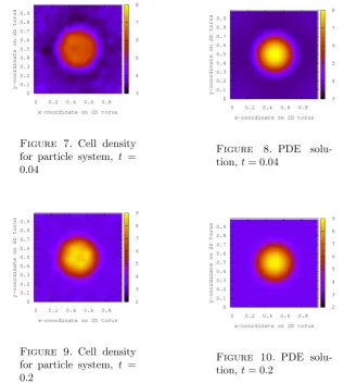
Figure 7. Cell density for particle system, t = 0.04

Figure 8. PDE

solu-tion,t= 0.04

Figure 9. Cell density for particle system, t = 0.2

Figure 10. PDE

solu-tion,t= 0.2

The simulations for the cell density exhibit an interesting phenomenon near the boundary of the support of the positive density of the chemo-attractant, which it-self is not visualized in the figures. Initially a ring of lower cell density forms around the area where the cells finally will concentrate due to positive chemotaxis, best vis-ible as the blue ring in Figures 2 and 4. This can be explained by particles jumping out of the region of this ring into the domain of positive chemical attraction where they get stuck due to their lower motility there. If they jump out of this domain again, then they may not move very far away from it by random motion. This leads to a density profile which is a non-monotone function of the distance from the centre. For longer times this effect vanishes, however, and the density approaches the steady state, which (in the hydrodynamic limit as N → ∞) is numerically in-distinguishable from the solution of the PDE at timet = 0.2 shown in Figure 10. Initially, the fluctuations of the initial condition dominate in the simulation of the particle system, which explains the rather large difference to the deterministic so-lution of the PDE. Averaging over several realizations of the particle system would lead to closer resemblance between the two.

not have stationarity in this case but convergence towards a stationary random variable. Now we simulate only the respective particle model, since the solution for the limiting PDE would require more refined numerical schemes than given above, because now blow-up phenomena may occur.

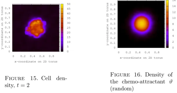
Our example here is the following, let us consider a zero range process within the range of so-called condensation. Specifically, we consider a ZRP with a constant jump rate g(n) = g0 for all n > 0. As soon as ϕ > g0, the partition function Z

defined in (2.3) does not converge and the corresponding grand-canonical measure (2.2) does not exist. As shown in [22, 23], for large enough densities the particles tend to concentrate on only a few sites with the lowest exit rate. However, in this case, this behavior is not due to the reinforced interaction of the cells and the at-tractive chemical molecules, but instead it is solely due to the stochastic properties of the ZRP. Such strong localization effects may relate to finite time blow-up of solutions of related limiting objects.

Figs. 11–15 show the results of simulations for this model with N= 100, g(n) = 3, and all other parameters given as before, i.e. uniform initial configurationη(x) = 4, χ0= 2,ν = 0.5 andϑgiven in (4.3) with final averaging over the empirical measure

with radius 0.05. In fact, this radius can be seen explicitly at points where many particles have clustered in the figures below. Figure 16 shows the random density of the chemo-attractant in order to compare with the location of the cell aggregate.

Figure 11. Cell

den-sity,t= 0.008

Figure 12. Cell

den-sity,t= 0.04

Figure 13. Cell

den-sity,t= 0.1

Figure 14. Cell

Figure 15. Cell

den-sity,t= 2

Figure 16. Density of the chemo-attractant ϑ (random)

If the total density in the system is high enough, we expect that eventually a fi-nite fraction of all particles will concentrate on the site with the highest number of chemical molecules.

5. _{Concluding remarks}

In this paper we derived the first equation of a general class of chemotaxis systems via a hydrodynamic limit of a stochastic lattice gas. The attractive chemical envi-ronment is prescribed in our case and assumed to be random and stationary, with a slowly varying mean. The situation of very strong clustering of the particles on single lattice sites is excluded in our theory, although this phenomenon can happen during selforganization of chemotactic particles in certain situations, and then it is of important biological relevance, like for the slime mold amoebaeDictyostelium discoideum. It would be interesting to be able to derive the full chemotaxis system from a hydrodynamic limit. Technically this is more challenging and methods of scale separation might play a role here.

Acknowledgements

Major parts of this work were done while D.M. and A.S. were working at the University of Heidelberg. This work was finished while A.S. took part in the CGP-program, 2015 at the Isaac Newton Institute, Cambridge.

References

[1] R. A. Adams and J. J. F. Fournier,Sobolev Spaces. Elsevier (2003)

[2] W. AltBiased random walk models for chemotaxis and related diffusion approxima-tions, J. Math. Biol.9(1980), no. 2, 147–177.

[3] L. Avena, T. Franco, M. Jara, F. V¨ollering,Symmetric exclusion as a random envi-ronment: Hydrodynamic limits, Ann. Inst. H. Poincar´e Probab. Statist.51(2015), no. 3, 901–916.

[4] C. Bahadoran, H. Guiol, K. Ravishankar and E. Saada,Euler hydrodynamics of one-dimensional attractive particle systems, Ann. Probab.34(2006), no. 4, 1339–1369. [5] C. Bahadoran, H. Guiol, K. Ravishankar and E. Saada, Euler hydrodynamics for

attractive particle systems in random environment, Ann. Inst. H. Poincar´e Probab. Statist.50(2014) no. 2, 403–424.

[6] P. Billingsley, Convergence of probability measures, 2nd ed. (1999), Wiley Series in Probability and Statistics, John Wiley & Sons Inc., New York.

[8] S. Childress and J. K. Percus, Nonlinear aspects of chemotaxis, Math. Biosci. 56

(1981), no. 3-4, 217–237.

[9] P. Covert P. and F. Rezakhanlou,Hydrodynamic limit for particle systems with non-constant speed parameter, J. Statist. Phys.88(1997), no. 1-2, 383–426.

[10] A. De Masi, S. Luckhaus, and E. Presutti,Two scales hydrodynamic limit for a model of malignant tumor cells, Ann Inst. H. Poincare Probab. Statist. 43(2007), no. 3, 257–297.

[11] L. C. Evans,Partial Differential Equations, 2nd Edition, Graduate Studies in Math-ematics19, American Mathematical Society (2000).

[12] J. Fritz and B. T´oth,Derivation of the Leroux system as the hydrodynamic limit of a two-component lattice gas, Comm. Math. Phys.249(2004), no. 1, 1–27.

[13] P. Gon¸calves and M. Jara,Scaling limits for gradient systems in random environment, J. Stat. Phys.131(2008), no. 4, 691–716.

[14] S. Großkinsky and H. Spohn,Stationary measures and hydrodynamics of zero range processes with several species of particles, Bull. Braz. Math. Soc. (N.S.)34(2003), no. 3, 489–507.

[15] M. Z. Guo, G. C. Papanicolaou and S. R. S. Varadhan,Nonlinear diffusion limit for a system with nearest neighbor interactions, Commun. Math. Phys.118(1988), 31-59. [16] W. J¨ager and S. Luckhaus,On explosion of solutions to a system of partial differential

equations modelling chemotaxis, Trans. Amer. Math. Soc.329(1992), no. 2, 819–824. [17] M. Jara,Hydrodynamic limit of the exclusion process in inhomogeneous media, Dy-namics, games and science (II) 449–465. Springer Proc. Math.2, Springer, Heidelberg (2011).

[18] E. F. Keller and L. A. Segel,Initiation of slime mold aggregation viewed as an insta-bility, J. Theoret. Biol.26(1970), 399–415.

[19] C. Kipnis and C. Landim, Scaling limits of interacting particle systems. Springer (1999).

[20] A. Koukkous,Hydrodynamic behavior of symmetric zero-range processes with random rates, Stochastic Process. Appl.84(1999), no. 2, 297–312.

[21] A. Koukkous and H. Guiol,Large deviations for a zero mean asymmetric zero range process in random media, arXiv:math/0009110.

[22] J. Krug and P. A. Ferrari,Phase Transitions in Driven Diffusive Systems With Ran-dom Rates, J. Phys. A-Math. Gen.29(1996), L465–L471.

[23] C. Landim, Hydrodynamical limit for space inhomogeneous one-dimensional totally asymmetric zero-range processes, Ann. Probab.24(1996), no. 2, 599-638.

[24] T. M. LiggettStochastic interacting systems: contact, voter and exclusion processes, Grundleheren der Mathematischen Wissenschaften324, Springer (1999).

[25] S. Luckhaus and L. Triolo, The continuum reaction-diffusion limit of a stochastic cellular growth model, Atti Accad. Naz. Lincei CI. Sci. Fis. Mat. Natur. Rend. Lincei (9) Mat. Appl.15(2004), no. 3-4, 215–223.

[26] D. Marahrens,A hydrodynamic limit for a zero range process in a random medium with slowly varying average, Diplomathesis, University of Heidelberg (2008). [27] K. Oelschl¨ager,A law of large numbers for moderately interacting diffusion processes,

Z. Wahrsch. Verw. Gebiete69(1985), no. 2, 279–322.

[28] K. Oelschl¨ager,On the derivation of reaction-diffusion equations as limit dynamics of systems of moderately interacting stochastic processes, Probab. Theory Rel. Fields82

(1989), no. 4, 565–586.

[29] H. G. Othmer and A. Stevens,Aggregation, blowup, and collapse: the ABCs of taxis in reinforced random walks, SIAM J. Appl. Math.57(1997), no. 4, 1044–1081. [30] G. C. Papanicolaou and S. R. S. Varadhan, Boundary value problems with rapidly

oscillating random coefficients, Random fields, Vol. I, II (Esztergom, 1979) Colloq. Math. Soc. J´anos Bolyai27(1981), 835–873.

[31] T. Rafferty, P. Chleboun, S. Grosskinsky,Monotonicity and Condensation in Homo-geneous Stochastic Particle Systems, arXiv:1505.02049.

[32] F. Rezakhanlou, Hydrodynamic limit for attractive particle systems on Zd_{, Comm.}

Math. Phys.140(1991), no. 3, 417–448.

[33] R. Schaaf,Stationary solutions of chemotaxis systems, Trans. Amer. Math. Soc.292

(1985), no. 2, 531–556.

[34] F. Spitzer,Interaction of Markov processes, Advances in Math.5(1970), 246–290. [35] A. Stevens,Trail following and aggregation of myxobacteria, J. of Biol. Syst.3(1995),

no. 4, 1059–1068.

[37] A. Stevens,The derivation of chemotaxis equations as limit dynamics of moderately interacting stochastic many-particle systems, SIAM J. Appl. Math.61(2000), no. 1, 183–212.

[38] B. Toth and B. Valko, Perturbation of Singular Equilibria of Hyperbolic Two-Component Systems: A Universal Hydrodynamic Limit. Commun. Math. Phys.256

(2005), no. 1, 111–157.

[39] H.-T. Yau,Relative Entropy and Hydrodynamics of Ginzburg–Landau Models. Lett. Math. Phys.22(1991), no. 1, 63–80.

University of Warwick, Mathematics Institute, Zeeman Buildg., Coventry CV4 7AL, UK

E-mail address: [email protected]

Max-Planck-Institute for Mathematics in the Sciences (MPI MIS), Inselstr. 22, D-04109 Leipzig, Germany

Westf¨alische Wilhelms-Universit¨at M¨unster, Applied Mathematics, Einsteinstr. 62, D-48149 M¨unster, Germany