Development of a modelling framework for integrated catchment flood risk management

(1)

Development of a modelling

framework for integrated catchment

flood risk management

Peter William Metcalfe

A thesis submitted in partial fulfilment of the requirements of the University of Lancaster for the degree of Doctor of Philosophy

(2)

Authorship declaration

(3)

Acknowledgments

This work was funded by the JBA Trust (project number W12-1866) and the European Regional Development Fund, with funding managed by the Centre for Global Eco-innovation (CGE), project number 132.

With thanks to my supervisors Professor Keith Beven, Dr Barry Hankin and Professor Rob Lamb, the members of the Brompton Flood Group, and all those involved in the Rivers Trust Life IP project (Dr Nick Chappell, Iain Craigen, David Johnson and Dr Trevor Page). Many thanks to the team at the CGE office, particularly the programme manager Dr Andy Pickard. Dr Mary K. Saunders helped devise the thesis plan and she contributed her professional GIS skills to Chapter 4.

Special thanks are due to the European Union, without which this work would have not been possible.

(4)

Abstract

Flooding is one of the most significant issues facing the UK and Europe. New approaches are being sought to mitigate its impacts, and distributed, catchment-based techniques are becoming increasingly popular. These employ a range of measures, often working with the catchment’s natural processes, in order to improve flood resilience. There remains a lack of conclusive evidence, however, for the impacts of these approaches on the storm runoff, leading to considerable uncertainty in their effectiveness in terms of mitigating flood risk.

A new modelling framework for design, assessment, and uncertainty estimation of such distributed, nature-based schemes is developed. An implementation of a semi-distributed runoff model demonstrates robustness to spatio-temporal discretisation. Alongside a new hydraulic routing scheme, the model is used to evaluate the impacts on flood risk of in-channel measures applied within an 29 km2_{agricultural catchment.} Maximum additional channel storage of 70,000 m3_{and a corresponding reduction of} 11% in peak flows is seen. This, however, would not have been insufficient to prevent flooding in the event considered.

(5)

The methodology can reflect the uncertainty in application of natural flood risk management with a poor or incomplete evidence base. The modelling results demonstrate the importance of antecedent conditions and of the timings and magnitudes of a series of storm events. The results shows the benefits of maximizing features’ storage utilisation by allowing a degree of “leakiness” to enable drain-down between storms. An unanticipated result was that some configurations of measures could synchronise previously asynchronous subcatchment flood waves and have a detrimental effect on the flood risk.

(6)

GLUE Generalised Likelihood Uncertainty Estimation. A methodology for quantifying uncertainty by combining a variety of likelihood measures to score model outputs.. Multiple realisations of models configurations and parameters sample from prior distributions and scored according to one or likelihood functions.

(24)

Hydraulic conductivity The rate of movement of water per unit area per unit head gradient through a medium such as soil. Dimensions are [L]/[T] and typical units m/hr.

Hydraulic head The amount of energy per unit weight of a fluid. In hydrology and hydraulics expressed in units of length ([L]; m). In an open channel the head comprises potential (or elevation), velocity head from downstream movement and pressure head due atmospheric pressure.

Hysteresis In the context of hydrology, a relationship between two state variable such as capillary pressure and soil moisture that develops distinctly under wetting and drying conditions.

Implicit Describes a procedure for solving numerically an expression for state variables of a system at a particular point in space and time, where the solution scheme includes the current state.

Infiltration The vertical movement from the surface into the soil. Insolation Intensity of solar radiation on a surface (kW/m2₎

(25)

Macropores Large soil pores created, for example, from tree root voids and macroinvertebrate activity, animal burrows, and desiccation, that can act as preferential pathways for infiltration and subsurface flow.

Monte Carlo (simulation) Model simulation employing many runs taking parameters sampled from random distributions.

Morphology The shape of a surface feature or river channel.

Network Width Routing Time delay histogram derived from distances of the points on the channel network, or on the hillslopes, from the catchment outlet.

NSE Nast-Sutcliffe Efficiency. A performance measure commonly used to determine the fidelity of a runoff simulation against observed flows. Frequently used as a likelihood measure in GLUE.

ODE Ordinary Differential Equation. A differential equation formulated in terms just one independent variable such as time.

Open channel flow Free surface flow at atmospheric pressure.

Orographic Describing precipitation caused by uplift due to relief. Overbank (flow) Storm flow that takes place outside the usual river

(26)

PDE Partial Differential Equation. A differential equation formulated in terms of more than one independent variable such as time and distance. Examples include the Shallow Water Equations and the Saint Venant Equations.

Peds Aggregation of soils into irregular blocks separated by soil pores.

Pore Voids in the soil matrix between peds.

Potential evapotranspiration Abbreviated Ep. Dimensions [L]/[T] and typical units

mm/hr. The maximum theoretical rate of evapotranspirationgiven insolation and unlimited water supply to the root zone.

Projected coordinate reference system

A CRS where the values are projected from a plane onto the Earth’s surface and thus directions are preserved. Raster Format for values covering a two dimensional field

(usually a spatial plane) where the values are evenly spaced within a grid.

Rating Development of a rating curve for or a channel section or engineered hydraulic structure such as a flume.

Rating curve A relationship derived empirically between river stage and discharge.

Realisation A model whose parameters and inputs have been fixed to particular values and can produce predictions.

(27)

Riparian (zone) The area immediately around the river channel.

Saint Venant Equations A series of PDEs analogous to the Shallow Water Equations in one spatial dimension describing open channel flow.

Saturated zone The region in the subsurface where the soil is completely full and cannot contain any more water.

Semi-distributed A model where the spatial complexity is minimised by aggregating areas into Hydrological Response Units. SWE Shallow Water Equations. A series of equations derived

from the Navier-Stokes equations for fluid flow. They describe free surface movement of water across a plane, where the flow depth is much smaller than its extent and the assumption of a uniform velocity profile is acceptable. Combines mass continuity with energy conservation in order to produce three PDEs formulated in two spatial dimensions.

Spatio-temporal Describing a state or quantity that varies in both state and time.

Specific Describing a measurement given in terms of its value per unit area, also known as intensity.

(28)

Subcritical (flow) In terms of open-channel hydraulics, describing flow where the majority of the head is composed of potential energy.

Supercritical (flow) In terms of open-channel hydraulics, describing flow where the majority of the head is composed of kinetic energy due to the water’s movement.

Tarlweg Midline of a river channel

TBR Tipping bucket recorder. A common type of rain gauge that consists of a small container on a see-saw type arrangement. Once the bucket is filled with rain water the bucket tips and empties the container. Each time this occurs it is recorded, thus the rainfall rate can be estimated.

Transmissivity The rate of water transmitted per unit contour per unit head gradient. Dimensions are [L]2_{/[T] and typical units}

m2_{/day or log(m}2_/hr).

Unsaturated zone The region in the subsurface where some of the soil pores have spare capacity.

Water table See saturated zone.

(29)

Chapter 1. Introduction

1.1. Overview

Flooding is the most damaging natural hazard, in terms of its economic impacts, facing the UK and the rest of Europe (EEA, 2011). The 2007 summer floods in the south of England caused damage of around £3.2 billion (EA, 2010) and the costs of 2013-2014 winter storms were at least £1.3 billion (EA, 2016). Those of the 2015-2016 floods are likely to exceed £1.5 billion (Marsh et al., 2015-2016). Floods are the most common weather-related disasters worldwide, and in 2011 the worldwide cost of flooding stood at around $24 billion (IPCC, 2014)

Across Europe there were significant floods in 2002 (Danube and Elbe) and in 2005, affecting mainly Austria, Germany, Romania and Switzerland (Kundzewicz et al., 2013). In 2006 and 2009 the Danube and Elbe were again affected and in 2010 the Central European Floods caused further damage in Poland, the Czech Republic and Hungary (EEA, 2011; Kundzewicz et al., 2013). Associated economic losses are estimated at €52 billion (EEA, 2011).

(30)

Flooding is likely to increase globally with predicted climate change (Delgado et al., 2010; Hirabayashi et al., 2013; IPCC, 2014). In Western Europe climate-change models indicate increased winter rainfall totals and lower but more intense summer rainfall, with much of the change projected to come within the 2020s (Ramsbottom et al., 2012; IPCC, 2014; Westra et al., 2014). Some studies suggest that in the UK the annual cost of flooding could rise from £1.2 billion at present to between £1.6 billion and £6.8 billion in 2050 (Ramsbottom et al., 2012).

Flooding can be defined as “the temporary covering by water of land not normally covered by water.” (EU, 2007). There are a number of causes of flooding (Dadson et al, 2017). Pluvial flooding is the result of rainfall intensity exceeding the infiltration capacity of the subsurface, with the excess flowing overland. Fluvial flooding occurs when discharge within a river reach exceeds its conveyance and overtops its banks. Coastal flooding is a consequence of extreme tides, weather and erosion. Overloading of artificial drainage is also referred to as Combined Overflow Discharge (COD). Groundwater flooding occurs at points, particular hollows, where the water table rises to the surface after prolonged recharge.

(31)

the U.K produced in response to the serious floods of 2007. The EA has incorporated many of the suggestion in the Review into its Flood Risk Management strategy (EA, 2012), in particular its recommendation to work with natural processes in order to reduce flood risk.

1.2. Traditional Flood Risk Management (FRM)

Conventional approaches to fluvial flooding often involve hard-engineered downstream defences that increase effective channel conveyance, These may be combined with artificial storage upstream to retain runoff and release it in a controlled fashion. Engineered defences can be designed to meet a rating specification expressed in terms of their ability to withstand and contain an event with a given annual exceedance probability (AEP), typically 1 in 100 years or 1%. The AEP is the nominal probability that such an event will occur in any given year.

Urbanisation is expanding the area under threat and other changes in land use are anticipated to increase the risk of flooding (Wheater & Evans, 2009). In December 2015 in Carlisle in Cumbria, defences upgraded to withstand a so-called “1 in 200 year” event were overwhelmed by a 1 in 1000 year event (Marsh et al., 2016).

(32)

1.3. Catchment based approaches to FRM

Integrated, Catchment-Based Flood Management is increasingly being applied (CBFM, Dadson et al., 2017; Lane, 2017). This aims to increase resilience to floods through upstream widely-distributed interventions, possibly in conjunction with downstream defences. It includes techniques to decrease fast runoff, for example by changes in land management to increase infiltration or by disconnection of surface flow pathways from the channel. Other measures are the addition of runoff storage on hillslopes through the introduction of soft-engineered features such as bunds; or by providing space on the floodplain for overbanked storm flows. The overall aim is to retain storm runoff in the headwaters and release it more slowly than for the unmodified catchment and thus reduce peak flows in affected areas downstream.

One variety of CBFM is an approach known as Natural Flood Management (NFM) that meets its aims by enhancement of the natural processes within the catchment. Natural flood management “… involves techniques that aim to work with natural hydrological and morphological processes, features and characteristics to manage the sources and pathways of flood waters” (SEPA, 2016). Associated measures such as tree-planting can reduce water yield through increased evaporation. NFM can enhance ecosystem services across the catchment and help meet the chemical and ecological status requirements of the Water Framework Directive (Nisbet et al., 2011; Barber & Quinn, 2012; Iacob et al.; 2014; EEA, 2016).

(33)

uncertainty in the hydrological impacts and hydraulic performance of soft-engineered measures. Realistic modelling approaches that incorporate uncertainty are essential for strategic placement of such measures to optimise their benefits in terms of flood risk mitigation, and to identify where their locations could slow flow inappropriately and potentially increase flood risk. The implementation of the European Floods and Water Framework Directives has further increased the importance of methodologies for development of the required river basin management plans.

The complexity of fully-distributed river and runoff models limit their application to larger catchment scales. Conversely, the crude spatial resolution of lumped or statistical catchment models significantly limits their use for assessment of detailed flood measures. There appears to be scope for an intermediate scale modelling approach that can incorporate sufficient detail to simulate both widely-distributed arrays of smaller features and larger scale measures but that is sufficiently simple that it can be used within a uncertainty estimation framework.

1.4. Project overview

Aims and objectives

The overall aim of the project is to develop a scalable and computationally efficient computerised modelling framework for the design and assessment of distributed, soft-engineered approaches to flood-risk management.

Research questions that will be addressed include:

(34)

2. What are the effects of antecedent conditions and timings and magnitude of sequences of storm events on the effectiveness of NFM schemes?

3. Do NFM measures have any mitigating effect through extreme events?

4. Do the synchronisation or desynchronisation of subcatchment flood waves have significant effects on the effectiveness of distributed FRM?

5. How best can uncertainty and “fuzzy” evidence be reflected in the application of natural flood mitigation measures?

Objectives to help answer these questions and meet the project aim are:

1. To develop a scalable, robust, computationally efficient runoff model

2. To develop a model which can simulate in-channel features and their combined effect on the storm flows within the channel network

3. To develop a scalable surface routing method that can represent the effects of measures to intercept overland storm runoff

4. To develop a framework for modelling the effects of widely-distributed hillslope interventions at a catchment scale

5. To apply the model developed in objective 4 within an uncertainty estimation framework.

Approach

(35)

catchments ranging in size from just under 100 km² to over 220 km², displaying a combination of upland, marginal grazing and arable land with urban areas at their outlets.

The models described in the project were, in general, implemented in the R language and environment. This has been applied in a number hydrological applications (e.g. Buytaert, 2008; Mehrotra et al., 2015; Turner et al., 2016). It was also considered appropriate as:

• It is open source and has a wide user community

• There are many “packages”, self-contained third-party modules delivered via the Comprehensive R Archive Network (CRAN). Packages are accepted on CRAN only after passing rigorous QA and cross-platform compliance. Extensive use were made of third party modules such as those listed below.

• It has fully-featured packages for analysis, manipulation and presentation of data, and time series, particularly useful for hydrological contexts, e.g. xts (Zeileis, Grothendieck, 2005) and data.table (Dowle et al., 2014).

• It has packages for spatial analysis and wrappers to spatial libraries such as GEOS and GDAL (rgeos, Bivand & Rundel, 2014; rgdal, Bivand et al., 2014) .

(36)

Scope

There are attempts to model flood risk globally using subgrid scale parametrisations of remotely-sensed elevation and hydrometric data (e.g. Yamazaki et al., 2011). Availability of hydrometric data for input to, and calibration of such models is in general restricted. The limited spatial resolution of data such as that of the Shuttle Radar Topography Mission (SRTM) means that it will be difficult to represent the small-scale flood mitigation interventions proposed for natural flood management. In the UK high resolution topographic and hydrometric data are readily available from sources such as the Environment Agency. This study will, therefore, use catchments from the UK. The techniques developed, however, will be broadly applicable to temperate catchments worldwide, subject to suitable data being available. Pluvial and fluvial flooding only will be considered.

1.5. Document structure

The thesis is comprised of this introduction, a literature review of modelling of catchment processes and natural flood mitigation strategies (Chapter 2), and four multi-author papers, on three of which the thesis author is first author. A summary of the author’s contributions to each of the included papers can be found in the supporting statement preceding each paper. Three appendices detail the mathematics behind the models developed.

(37)

Dynamic TOPMODEL: A new implementation in R and its sensitivity to time and space steps

This describes a new, open source, implementation of a semi-distributed model developed to simulate runoff and soil moisture deficits. The paper describes its underlying methodology, modular structure and an application to a simulated landscape and a small (3.65km²) catchment in Wales, UK. Various spatial and temporal discretisations are applied to a single calibration period. The implementation demonstrates robustness to the various schemes and convergence to a limiting output. Appendix 1 details the flux calculations and new surface routing method introduced in this implementation.

A modelling framework for evaluation of the hydrological impacts of nature-based approaches to flood risk management, with application to in-channel interventions across a 29 km² scale catchment in the United Kingdom

(38)

Appendix 2 details the hydraulic routing scheme for channel routing. and Appendix 3 suggests formulations for the hydraulic characteristics of selected in-channel flood mitigation measures.

Strategies for testing the impact of natural flood risk management measures.

This chapter describes a four month long project undertaken for the Rivers Trust in liaison with Lancaster Environment Centre and JBA Consulting. The author acted as research associate and developed the computer model with which the detailed modelling was undertaken. The project aimed to investigate the potential for applying a nature-based approach for flood mitigation across the headwaters of three Cumbrian catchments badly affected by the extreme storm events of the winter of 2015-2016. The runoff model described in Chapter 3 was further developed to allow simulation of the effect of the addition of various types of widely-distributed hillslope interventions for flood mitigation. These include peat restoration, soil structural improvements, tree-planting on hillslopes and riparian areas, and deepening of existing accumulation areas to provide detention storage area for surface runoff.

(39)

Simplified representation of runoff attenuation features within analysis of the hydrological performance of a natural flood management scheme

A measure simulated in the project described in Chapter 5 was the insertion of runoff attenuation features (RAFs) intended to intercept and store overland storm runoff. The new surface routing module developed in Section A.1.4 was modified to allow modelling of these features. This chapter describes the modelling using this approach, through the storm period from the previous study, of approximately 4500 of such features across the 228km² headwaters of the Eden, Cumbria, UK.

The study applies an uncertainty estimation framework to the simulated runoff for unmodified and intervention cases. Features with a number of different “leakiness” characteristics are applied. Some conclusions are drawn on the effects of different drain-down times across extreme events such as those studied. The chapter discusses whether the simplified representation is valid and suggests some experimental approaches to determining the behaviour of such features and their effects on the catchment response.

(40)

(41)

Chapter 2. Review of literature and modelling of

catchment processes

2.1. Introduction

Models play an important role within catchment management (Jakeman & Letcher, 2001; Lerner et al., 2010). Beven (2012) provides a comprehensive review of catchment model development, from the formulation of a perceptual and conceptual structure to implementation, calibration and validation.

2.2. Modelling approaches

Beven (2012) categorises models as “lumped-conceptual” or “physical / process-based”. In the first case, the catchment, its processes and internal states are treated as a whole and modelled statistically or probabilistically. In physical, or process-based, models the internal processes are modelled explicitly according to physical laws and applied to update internal state variables over time.

A simple example of a lumped-conceptual models is the Unit Hydrograph technique, which considers the response of the catchment to a single unit of effective rainfall as an additive property on which linear algebraic operations can be performed in order to derive its response to more complex hyetographs.

(42)

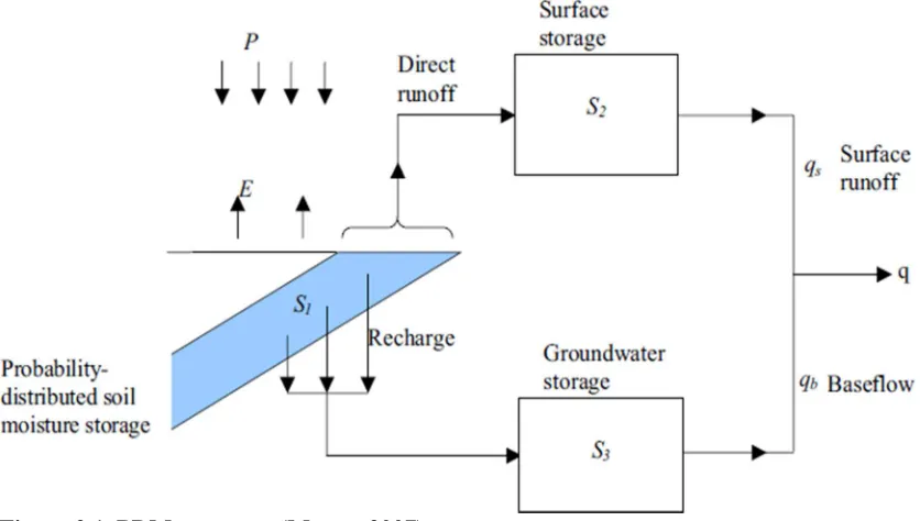
determined by the PDF, of the excess over capacity of stores that have filled. The distribution is updated according to the incident precipitation, runoff and evapotranspiration of the likely transfer of storage between elements.

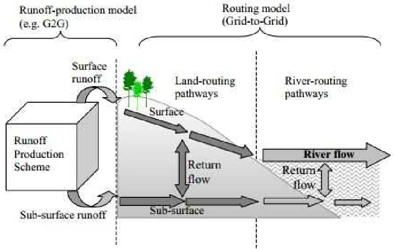
The PDM approach is flexible and scalable and has been used as the hydrological model underlying other applications such as Grid-to-Grid (G2G; Bell & Moore, 1998; Bell et al., 2007).

Increased spatial resolution is introduced in semi-distributed models. These attempt to simplify the complexity of the problem domain by grouping together areas with similar properties. They may then be treated each as a conceptual store known as a hydrological response unit (HRUs) or hydrological similarity unit (HSU) whose constituents can be partially mapped back into space.

[image:42.595.108.526.160.397.2]

(43)

TOPMODEL (Beven and Freer, 2001a) allow for a more general grouping approach that can, for example, take into account hydrologically-significant heterogeneity within the catchment such as land cover or soil type.

INCA (Integrated Nitrogen model for multiple source assessment in Catchments; Whitehead et al., 1998) is a water quality model that incorporates a semi-distributed runoff component. Here landscape units are identified with the areas draining to individual reaches in the river network.

In spatially-explicit, fully-distributed models, state variables are maintained across the catchment at points that can be mapped directly into actual space. Such models are usually physically-based (Beven, 2012). Examples include the Système Hydrologique Européen (SHE, Abbott et al., 1986) and later variants including MIKE-SHE (Refsgaard & Storm, 1995). HydroGeoSphere (Therrien et al., 2010; Brunner & Simmons., 2012) is a recent example that makes use of modern parallel computation techniques to solve for three-dimensional fluxes in the unsaturated zone. HydroGeoSphere was developed from the FRAC3DVS subsurface transport model (Therrien & Sudicky, 1996) with the addition of a 2D component for overland flow routing.

(44)

Multi-scale models apply different treatment of space and time to distinct components of the system. A coarse spatio-temporal discretisation or static risk or opportunity mapping stage may be applied in order to identify areas that have a significant impact on the system response. An example of such a models is SCIMAP (Reaney et al., 2007). SCIMAP uses a network connectivity index calculated from flow distances of areas from the channel network (Lane et al., 2004) combined with the Topographic Wetness Index in order to identify critical source areas (CSA, Heathwaite et al., 2005) that are likely to both provide a source of pollution and are connected to the channel. A spatially-explicit model, Connectivity of Runoff Model (CRUM, Reaney et al., 2007) is then applied to those areas to estimate the dynamic solute mass flux from the critical areas to the channel network.

2.3. Uncertainty and equifinality

[image:44.595.125.514.87.333.2]

(45)

catchment’s internal state (Beven, 1989, 1993, 2000). However, it is those states and their response to modification that will be of most interest to a catchment manager investigating potential flood mitigation interventions.

A typical approach is to apply model(s) that represent the catchment processes mathematically and to link their outputs to produce estimates of the quantities of interest. Any observational data available are used to determine the likely parameters of these models by reconstructing or calibrating against historical flows and states; these are then applied to predict the response of the system to future inputs. For example, a rainfall runoff model will take time series of rainfall and evapotranspiration in order to predict the discharge at the catchment outlet. Given a set of observed discharges, the parameters of this model will be adjusted or calibrated so that its outputs match the observations. Given residual errors in the model, this will help to predict the catchment response to different inputs, such as sets of spatially coherent designed extreme rainfall events and to assess the impact of interventions on the runoff.

In this approach the model is considered to be correct. Epistemic errors (lack of knowledge of the processes involved) introduce significant uncertainty(see e.g. Beven, 1989; 2009). In addition, observations of environmental data are more uncertain than for engineered systems (Jakeman & Hornberger, 2003), errors may vary non-linearly with state and be non-stationary over time (Beven, 2006). Given this inherent uncertainty, even if a perfect theoretical representation of the catchment were available, it is doubtful whether calibration could fix a “true” set of parameters (Beven, 2006; Jakeman & Hornberger, 2003).

(46)

which calibration data are scarce or non-existent (Beven, 1989; Jakeman & Hornberger, 2003). Furthermore, Beven (1993, 2006) observes that different choices of model structure and parameter sets can give rise to similar, and acceptable, predictions of the observed outputs. Such “equifinality” means that in practical terms the components of a catchment system may have to be treated as “black boxes”, with only input and output states known within the limitations imposed by observational error. In practice, the physical states within grid cells of fully-distributed models are not completely defined, and each could in fact be considered an individual lumped-conceptual model (Beven, 1989, 1993).

The Generalised Likelihood Uncertainty Estimation (GLUE) methodology (Beven & Binley, 1992 and 2014) accepts the equifinality of parameter sets and formalises this approach. It provides a framework in which behavioural parameter sets, in that they replicate adequately the response of the system to observed inputs, are identified within multiple (Monte Carlo) runs of the model. One or more likelihood measures may be used and combined to produce a single metric. A simple function is triangular across an interval defining the acceptable range of the observable: the midpoint value is unity and those outside the limits zero, and values are linearly interpolated between these points.

(47)

Examples of applying GLUE to FRM modelling are found in 0 and 6.

2.4. Data for hydrological models

Depending on their formulation, hydrological models will require meteorological data (precipitation, evapotranspiration), catchment elevations and boundaries, and location and properties of river reaches. They may require other hydrometric data such as rated discharges for calibration. Physically-based, distributed models may be required much more detailed information such as surface effective roughness, soil water retention characteristics and hydrological conductivity. These may be difficult to measure, particularly at extensive spatial scales, and is open to question how well the measurement of a physical value at a single point can scale to the size of a grid element (Beven, 1989).

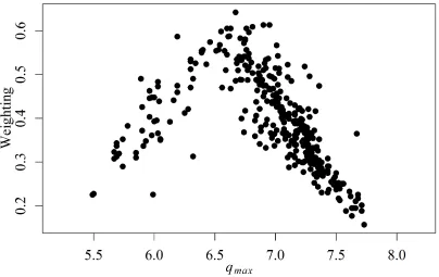
Figure 2.3. Example “dotty” plot showing the overall weighting of realisations against one observable from a flood simulation, the peak discharge qmax. This must lie within the

[image:47.595.111.515.73.328.2]

(48)

Topographic data

Many physical models use digital elevation data in order to infer the spatial variation of hydraulic gradient; a common assumption is that this is approximately parallel to the local surface. This is most appropriate for hillslopes with thin soils and impermeable bedrock. It should be noted, however, that the form of the bedrock can often have a greater impact on flow pathways than that of surface topography McDonnell et al. (1996).

Geo-referenced elevation data are widely available and generally provided as gridded rasters in GEOTiff or ASCII format, for example. Buildings and vegetation canopies are removed algorithmically from these data to produce a digital terrain models (DTM), the ground surface elevation. Elevation data that include buildings and vegetation yield a Digital Surface Model (DSM) and are more appropriate for mapping of surface water flooding in urban areas, for example. Datasets such as the ASTAR-GDEM (Advanced Spaceborne Thermal Emission and Reflection Radiometer Global DEM) and SRTM (Shuttle Radar Topography Mission), obtained through remote-sensing ,provide world-wide coverage at horizontal resolutions of between 30 and 50m. Data at 10m resolution are available for the entire UK via the OS Digimap datasets, accessible via the EDINA service. Intermap provide the NEXTMap commercially-licenced data that include UK-wide 2m DTMs / DSMs. As of 2015 the Environment Agency have made available for public use their LiDaR (Light Detection & Ranging) elevation data. Coverage in 2009 was 72% of the UK. Horizontal resolutions range from 2m to 25cm and elevation accuracies are up to 5cm (EA, 2009).

(49)

2008). The Integrated Hydrological Units (IHU, Kral et al., 2015) and Ordnance Survey OpenRivers archives provide catchment boundaries and rivers networks across the UK.

Indices of similarity calculated from gridded data are likely to be sensitive to the grid size (Saulnier et al., 1997). Gridded data with resolutions of over 100m are considered

too coarse for use in hydrological models. (Beven, 2012).

Land use, land cover and soil types

Spatial data on land cover may be required by physically-based models with interception stores based on vegetation (and by inference, canopy type). Semi-distributed models such as SWAT allow for grouping of landscape units according to the land cover and vegetation type.

The Hydrology of Soil Types (HOST, Boorman et al., 1995) is a 1 km resolution raster dataset. It classifies the soils of the UK into 29 types according to hydrological characteristics that affect the catchment-scale response. These include SPRHOST, the Standard Percentage Runoff or proportion of incident rainfall that contributes to the fast response. Each grid cell in the raster indicates the predominant type within that area. The Flood Estimation Handbook (FEH; Institute of Hydrology, 1999) and Revitalised Flood Estimation Handbook (ReFH; Kjeldsen et al., 2005) employ catchment descriptors utilising values derived from predominant soil HOST classes.

(50)

The Land Cover Map (LCM; Morton et al., 2007) comprises a vector and 25m raster dataset covering the UK. The vector data indicate the predominant land cover in terms of one of 23 broad habitat classifications, such as broadleaved woodland, and the subcategory of that classification. The raster data indicate the likely habitat category within each 25x25m cell. One application of the LCM relevant to flood modelling is to identify areas of improved grassland where soil structure can be improved and thus reduce fast runoff.

The European CORINE land cover (CLC) raster map is remotely-sensed at a resolution of 100m and comprises 44 land cover classifications. CLC was last updated in 2012. The dataset can, for example, be used to exclude areas from application of NFM measures according to their proximity to certain land use types.

2.5. Components of physically-based models

(51)

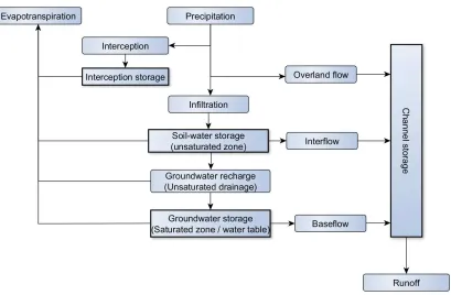
Singh (1995), Shaw et al. (2011), and Beven (2012) provide reviews of widely-used models and their implementations of the components of the Freeze-Harlan template. This section will review these and the corresponding literature.

Evapotranspiration and interception

Evapotranspiration is the removal of water from the surface or near-surface, through a combination of evaporation from the soil and plant transpiration. It accounts globally for 60% of the water lost from the land surface into the atmosphere (Yamazaki et al., 2011). In temperate climates it will make up 25 to 65% of the output from the catchment. In hot climates with seasonal rainfall it can make up the overwhelming majority of the water lost from the system (Shaw et al., 2011).

[image:51.595.114.523.66.334.2]

(52)

greater than or equal to the actual evapotranspiration Ea (or Et) and will depend on isolation, relative humidity, wind speed and soil moisture content.

The Penman-Monteith relationship (Montieth, 1965) can be used to calculate actual evapotranspiration from the interception and near-surface plant uptake stores (root zone) as

= 3.6 ∗ 10 ∗ ∆ +

Δ + ! 1 + "_#$

(Eqn. 2.1)

with = net radiation input (kW/m²); ∆ = gradient of saturation vapour pressure

against temperature (kPa/ºC), % and % the aerodynamic and canopy resistances respectively (s/m), ρ the density of air (kg/m³), λlatent heat of vaporisation for water (kJ/kg), _&_' the vapour pressure deficit (kPa), ₍₎ the specific heat of air (kJ/kg) and γ the psychrometric constant (kPa/ºC).

The current version of SWAT allows the use, depending on the meteorological data available, of the Penman-Monteith, Priestley-Taylor (Priestley & Taylor, 1972) or the Hargreaves method (Hargreaves & Samani, 1982). The second two methods require only temperature and radiation input. In addition to the Penman-Monteith equation, MIKE-SHE and HydroGeosphere can use the Kristensen-Jensen scheme (Kristensen and Jensen, 1975) in order to estimate interception and evapotranspiration.

(53)

1967; Rutter et al., 1971). Rates for deciduous trees vary through the year depending on their leaf cover: a study from southern England found interception losses of 29% and 20% in the leafed and leafless periods, respectively (Herbst et al., 2008).

Models such as SHE and the Institute of Hydrology Distributed Model (IDHM: Beven et al., 1987; Calver and Wood, 1995) include an interception store from which evapotranspiration is removed and the remainder passed on to the surface by throughfall. A Rutter interception model (Rutter et al., 1971) is used. The canopy storage C ([L], mm) satisfies the relationship

*+

* = , − ./0 123 (Eqn. 2.2) where S is the canopy storage capacity (mm), b (mm-1) and k (-) are drainage parameters, and Q (mm/hr) is the recharge rate due to rainfall less evapotranspiration, scaled by the proportion of ground obscured by vegetation.

TOPMODEL and Dynamic TOPMODEL implement a simple interception and “root zone” filled by incident rainfall and from which actual evapotranspiration in removed at a rate proportional to the potential as that time step divided by Srz.max ([L]; mm), its maximum capacity:

= ).₄4 5 5,7 8

(Eqn. 2.3)

(54)

),9 = ):1 + ;< => ?_{365 − 0.5BCD}@ (Eqn. 2.4)

If the insolation is taken to also vary sinusoidally through daylight hours a time series of potential evapotranspiration at a time t after sunrise can be calculated from the day length at the catchment's latitude.

Precipitation

Rainfall data may be obtained at multi-instrumented AWS or at individual gauges of varying design. Radar provides good estimates for spatial extent of rainfall but is less accurate in determining its quantities. Many meteorological data are recorded at automatic weather stations (AWS) or manned stations. The Met Office Integrated Data Archive System (MIDAS, Met Office, 2012) contains many of these data collected across the UK from 1853 to the present. Temporal resolutions found in the MIDAS dataset range from 15 minutes to hourly, daily, weekly and months.

(55)

Designed rainfall data can be useful for testing models and for rating flood defence schemes against events of known AEP. The SWRRB (Simulator for Water Resources in Rural Basins, Williams et al., 1985) applies a statistical approach to simulate daily rainfall input. The probability of rain given rain the previous day for the month and monthly averages are supplied for the basin and the series generated by a stochastic first-order Markov Chain model. Keef et al. (2013) provide a method to generate set of spatially-distributed rainfall events.

Snowmelt contributes some input to systems in higher latitudes and mountainous areas but in the UK is of less importance (Shaw et al., 2011). The accuracy of rainfall data in upland regions may be affected when collecting devices are covered by snow (e.g. Kirby et al., 1991). Calculation of snow melt equivalent to liquid precipitation is complex but a more straightforward approach is incorporated in SHE and variants . The amount of melt input M (mm/day) to the subsurface as E = E_F G − G₀ , where Ta is the air temperature (Cº) and Tb a reference temperature with Ta > Tb and E_F a factor appropriate to the aspect, region and season. When _G₀ _{= 0}, _E_F is known as the degree-day factor (Linsley, 1943).

SWAT incorporates an empirical snow melt component that provides input when the temperature of second soil layer rises above freezing, hence E = G 1.52 + 0.54. G_J , with G_J the snow pack temperature in degrees celsius.

Infiltration

(56)

*K

* =*L ?M* *K*L + NB (Eqn. 2.5)

where θ is the specific soil moisture content, z the depth below the surface (m), K the hydraulic conductivity (m/hr) and the soil water diffusivity _{M K = N}OP

OQ (m2/hr). General solutions are not available and it must be solved by numerical means and applying the appropriate boundary conditions.

The Green-Ampt Equation (Green & Ampt, 1911) is particular solution of the Richards Equation allowed by assuming a sharp boundary at a depth zf (mm) between an upper saturated region and soil at some initial wetness. The vertical (downwards) rate of infiltration f ([L]/[T], mm/hr) is:

R = NJ ST _L+ UF

F + 1$ (Eqn. 2.6)

where t (hr) is time after the start of infiltration, S_T (mm) the depth of ponded water on the surface, N_J ([L]/[T], mm/hr) the saturated hydraulic conductivity and U_F a parameter that relates to the capillary potential gradient across the wetting front. It can also be formulated in terms of the capillary drive ₊_V _{= U}_F_{WKX − K}_Y_Z (mm) where _KX is the field saturated soil moisture content (-) and _K_Yits initial state.

More straightforward infiltration formulas have been derived experimentally, such as the Horton Infiltration Equation (Horton, 1933) or by analytical solutions of simplifications of the Green Ampt equation. Examples of the latter include the Philip Equation (Philip, 1957) that makes use of the soil sorptivity s, ([T], hr) which must be found empirically:

R = ;

(57)

A storage-based formulation developed by Kirkby (Kirkby, 1975) is used in the CRUM model and the first version of TOPMODEL (Beven & Kirkby, 1979) and gives an explicit expression for the infiltration in terms of the current soil moisture

R = +\_K (Eqn. 2.8)

where a and b ([L]/[T], mm/hr) are empirically-determined parameters for the soil type.

In a later version of TOPMODEL the infiltration rate is simply taken to be the precipitation excess, the rainfall intensity minus any evapotranspiration, and water absorbed by spare capacity in the “root zone”.

Unsaturated zone drainage (water table recharge)

The one-dimensional Richards Equation for gravity drainage can also be expressed in terms of the capillary (pressure) potential _U ([M], Pa) and soil-water capacity ([L]-1₎ + =OQ_OP and R ([T]-1) a specific recharge / loss term due, for example to root zone

uptake, evapotranspiration or direct input, with z again positive in the vertical downward direction:

+*U_{* =}*N_{*L +}_{*L ?N}* *U_{*LB +} (Eqn. 2.9)

(58)

*K

* = ]. ^]_ + (Eqn. 2.10)

TOPMODEL uses a simpler approach that estimates the unsaturated drainage rate `5(mm/hr) at a particular time as _cd3Jab , the ratio of the overall moisture deficit in the

unsaturated zone, _;_e5 (mm), to the total storage deficit S (mm) and a time delay constant ₉([T]/[L]; hr/mm). This is equivalent to a linear store with mean residence time of ₉ hours.

The assumption of Darcy-Richards flow in the near surface for soils displaying macropores (large continuous voids) and preferential flows has been called in question by Beven & Germann (1982, 2013), amongst others. These macropores may allow direct recharge of the subsurface with little interaction with the soil matrix and spatial heterogeneity of flow pathways not well accounted in a framework that treats the soil as a continuous porous medium.

Saturated zone (water table)

As the movement of water downslope through the soil is slow, the Reynolds number will be less than unity. Most physically-based models therefore ignore changes in momentum when routing hillslope subsurface runoff.

The main axis of flow in the subsurface given by the direction of greatest hydraulic gradient. If the water table is taken to be approximately parallel to the local surface, this vector is perpendicular to the elevation contour lines.

(59)

*f

* + (*f*g = 4 (Eqn. 2.11) where x (m) is distance measured in the downslope direction, and S is the specific storage deficit (mm). The wave velocity, known as the celerity, is _{( =} Oh

O3 (L/T; m/hr), which may be much in excess of the flow velocity (Beven, 2010; Davies & Beven, 2012; McDonnell & Beven, 2014)

A kinematic approach is taken to routing flow between the gridded hillslope elements in G2G. Dynamic TOPMODEL also uses a kinematic routing procedure, except that this is now applied to route flow between the response units. The proportion of subsurface flow into downslope units, including themselves, is specified via a pre-calculated weighting matrix. This is determined from the topography, given an assumption of slope - hydraulic gradient equivalence. Contribution to channel flow is determined by the amount of hillslope flux redistributed by the matrix to a lumped “river” unit.

(60)

identify areas that have reached saturation according to the relationship for the storage deficit across a particular HRU (see Beven & Kirby, 1979; Beven, 2012)

MY = M + i =! − ? BC (Eqn. 2.12)

with γ equal to the mean value of the TWI ([ln(L2_{)]; ln(m}2_{) ) and}_M_{([L]; m), the mean} deficit across the catchment. If _M_Y_{<= 0} then the corresponding area is taken to be contributing runoff that enters the channel.

Dynamic TOPMODEL, by contrast, determines saturated excess runoff which it then. Areas of saturation excess are determined from the soil moisture deficits maintained for each unit and updated at each time step by the difference between downslope output and input from upslope units and unsaturated drainage.

The lumped conceptual model PDM determines the runoff by determining the excess over capacity of areas that have filled over the time step. These are scaled by their sizes relative to the catchment area, as determined by a PDF, to obtain the runoff over the time step. Storages are then updated by that runoff and the rainfall and evapotranspiration and storage transfer between areas is estimated probabilistically.

2.6. Surface runoff

In most catchments the largest proportion of runoff reaches the channel via subsurface pathways. Even in humid catchments with high rainfall where the ground is close to saturation much of the time, 80% of the runoff is subsurface or near surface (Chappell et al., 1999, 2006).

(61)

velocities are much lower, between 10 to 30 m/hr (Beven & Kirkby, 1979; Holden et al., 2008). Transport of sediment and erosion will largely take place during periods of surface runoff. In agricultural catchments overland flow is the primary means of transport of nutrients such as phosphorus (P) that cause ecological damage to water bodies (Heathwaite et al., 2005; Barber & Quinn, 2012; Thomas, et al. 2016). Efforts to mitigate nutrient over-enrichment will therefore identify areas with a propensity to produce this type of runoff (hydrologically sensitive areas or HSAs) that are hydrologically connected to the channel (critical source areas, CSAs) and seek to disconnect them through bund or other measures (Heathwaite et al., 2005; Thomas, et al. 2016; Roberts et al., 2017).

The significance of overland flow to flood risk is its contribution to fast response of catchment areas at or close to saturation. These areas are most likely to be close to the channel and will contribute to the rising limb of the hydrograph, bringing forward and intensifying the peak. FRM measures that reduce overland flow velocities will in theory slow this runoff so that it contributes to the falling limb instead.

Surface flow production

(62)

Modelling of surface runoff

Many hydrological models include a component to handle surface flow. There are also dedicated surface runoff models such as JFLOW (Lamb et al., 2009). A statistical approach is applied in the FEH and ReFH. In the former the Standard Percentage Runoff, SPRHOST, catchment descriptor determines the proportion of runoff taking surface pathways. Higher values of SPRHOST indicate that the soil class tends to produce more saturated overland flow as a consequence of lower hydraulic conductivities that inhibit drainage downslope. In the ReFH the Base Flow Index, BFIHOST, is used in conjunction with the PROPWET descriptor. PROPWET is the proportion of the catchment that is producing overland flow. 0 discusses the use of the SPRHOST descriptor in targeting areas suitable for flood mitigation measures designed to intercept or slow overland flow.

A topographically-based overland routing scheme is applied in TOPMODEL. Given a single overland flow velocity parameter vof, ([L/T], m/hr) the time taken for overland flow generated at any point in the catchment to reach the outlet is

l_mnF gY Y o

Ypq

(63)

areas, and applied to route any overland flow generated by the model to future predictions of discharge at the outlet.

Hydraulic schemes for routing surface flows are generally based on versions of the Navier-Stokes equations for an incompressible fluid. Depth of flow is usually taken to be much less than the horizontal length scale of the channel or region of flow. The vertical component of velocity is presumed to be small and the pressure gradient due only to depth (i.e.is hydrostatic). Given these assumptions, the velocity can be integrated through the depth of flow to give the depth-averaged the Saint Venant or Shallow Water Equations (SWE, see Murilloa et al, 2008; Lamb et al., 2009, and many others).

The SWE are often expressed as single vector equation expressing conservation of both mass and momentum in an orthogonal spatial basis _{r = s}_t#g with velocities in these directions (Lamb et al., 2009):

*u

* +*v u*g +*w u*t = x r, (Eqn. 2.14)

where

u = =S`S

SmC v = y

S` `z_{S +}1

2 {Sz S`m

| w = y

Sm S`m mz_{S +}1

2 {Sz

| (Eqn. 2.15)

(64)

JFLOW solves the SWE for each cell in a gridded raster to obtain flood extents, water velocities and heights. An explicit numerical scheme is used that applies appropriate boundary conditions from neighbouring cells, edges of the raster, or wetting and drying fronts. Any friction source terms calculated from the Manning surface roughness. Parallel and grid computing techniques are applied that allow the model to be applied over large spatial extents at high resolution. The surface is modelled as though impermeable, but a proportion of the rainfall can be removed to emulate infiltration, artificial drainage or other losses. These can be estimated, for example, from the ReFH BFIHOST descriptor relevant to the catchment.

Making use of the commercially-licenced NEXTMap 5m DSMs, JFLOW produced the Updated Flood Map for Surface Water (uFMfSW, EA, 2013) that assists in predicting flood risk across England and Wales. This is used by Local Lead Flood Authorities (LLFA) in order to meet the requirements of the European Floods Directive. Local planning authorities, utilities and businesses also make use of the maps to make strategic decisions. Designed events of AEP of 1%, 0.3% and 0.001 & are applied.

Approximations to the Shallow Water Equations can be derived from neglecting some of its terms (Beven, 2012). Their applicability depends on the importance of the conserved terms, the magnitude of the time and space variations in the system and the relative contributions of the source terms. If the friction is neglected in the source term then the gravity wave approximation results. This is suited for deep water such as lakes and is not generally used in overland routing. If the flow velocity depth at a particular point is taken to be slowly varying in time Oe

Oc and O}

(65)

If the flow velocities are taken to vary slowly in space the spatial derivatives of u and v can be neglected. The assumption is known as the diffusion wave approximation to the SWE. Flow is driven by any imbalance between the bed friction (friction slope) and the gravity acting on the water surface (Bradbrook et al., 2004). An explicit expression for the velocity vector v at each point across time can then be shown to be (Bradbrook et al., 2004):

~ = − S_|•L|z •⁄ •L_{ƒ •}_⁄ (Eqn. 2.16)

where n is the Manning roughness coefficient (T/[L]1/3; s/m1/3) and z the surface elevation above a datum and h the water depth, both in m. The Manning roughness coefficient is frequently utilised in surface and channel routing models. Typical values are in the range 0.03 for short grass to 0.15 for dense willow growth. Chow (1959) supplies tables of n values for artificial surfaces, common ground cover types and other natural surfaces. Effective roughness can vary considerably from these values depending on the depth of flow and the nature of vegetation (e.g. Holden et al., 2008).

The kinematic wave approximation to the SWE arises by further equating the friction slope with the bed slope within the source term. The water surface is everywhere then assumed equal to the local slope, •L = „_…. The velocity – depth ranges for which the kinematic wave formulation gives an acceptable approximation for surface flow routing is given by kinematic wave parameter (see Vieira, 1983).

Channel routing

(66)

modelled explicitly in space and time. Shaw et al. (2011) review a number of other methods for channel routing.

One hydrological approach, most suited for small catchments where hillslope runoff dominates over in-channel processes, is the Network Area or Channel width function method (Beven & Wood, 1993; Beven, 2012). Here the flow distance to the outlet for all areas in the catchment is calculated, and with a channel velocity applied across the network a time delay histogram produced. Earlier versions of TOPMODEL (such as that described by Beven & Kirkby, 1979) used the network area approach but at time t applied a non-linear wave speed determined from the current overall discharge Q (m3_{/s) at time}_t_:

( = †, ‡ _{(Eqn. 2.17)}

where

α

(m-1_{) and}

_β

_{(-) are parameters for the network. However, results from Beven} (1979) suggest that a fixed wave speed could be more appropriate as well as being more stable and later versions (including Dynamic TOPMODEL) apply a single parameter vchan (m/hr) across the entire simulation period.

Hydraulic routing approaches are found in many physically-based models. These are often one-dimensional approximations of the SWE with the x axis through the local midline and the velocity in the y direction, v, set to zero. Reasonably laminar flow is assumed Analogously to Eqn. 2.14 and Eqn. 2.15, the one-dimensional SWEs can be written

*u

* +*v u*g = ˆ g, (Eqn. 2.18)

whereu = s S

S`#andv =

S` `z_{S +}q