Algorithms or Actions? A Study in Large-Scale Reinforcement Learning
Anderson Rocha Tavares
∗1, Sivasubramanian Anbalagan
∗2,
Leandro Soriano Marcolino
2,
Luiz Chaimowicz
11
Computer Science Department – Universidade Federal de Minas Gerais
2
School of Computing and Communications – Lancaster University
[email protected], [email protected],
[email protected], [email protected]
Abstract
Large state and action spaces are very challenging to reinforcement learning. However, in many do-mains there is a set of algorithms available, which estimate the best action given a state. Hence, agents can either directly learn a performance-maximizing mapping from states to actions, or from states to algorithms. We investigate several aspects of this dilemma, showing sufficient conditions for learn-ing over algorithms to outperform over actions for a finite number of training iterations. We present synthetic experiments to further study such systems. Finally, we propose a function approximation ap-proach, demonstrating the effectiveness of learning over algorithms in real-time strategy games.
1
Introduction
Reinforcement learning aims at developing general agents, which learn by acting directly on the problem action space [Sutton and Barto, 1998]. However, as the state and action spaces grow large, learning agents struggle to attain high per-formance. On the other hand, many domains have existing algorithms, tailored to the specific problem, and an agent could rely on a pool of algorithms to act on its behalf [Rice, 1976]. Given limited computational resources, however, there is an important conflict: should welearn over actions, training a reinforcement learning agent to discover the best actions to take, or should welearn over algorithms, trying to discover the best algorithm to estimate the best action in each state?
Previous work on reinforcement learning with abstract ac-tions [Suttonet al., 1999; Dietterich, 2000] have shown that the optimal policy may not be attainable when learning over algorithms, although it may accelerate the reinforcement learn-ing process. However, it is still unclear when each method should be preferred. Additionally, having a pool of algorithms may still not enable one to directly apply reinforcement learn-ing techniques when the state space is also very large. In particular, Real-Time Strategy Games are a major challenge for Artificial Intelligence research, given their enormous action and state spaces [Onta˜n´onet al., 2013].
* A. R. Tavares and S. Anbalagan are both first authors.
In this work we establish the conditions where learning over algorithms is helpful, evaluating the sufficient strength of avail-able algorithms, the relation among algorithms and actions set sizes, and possible underlying algorithm creation processes. Synthetic experiments further develop our conclusions. Addi-tionally, we introduce a function approximation approach for Real-Time Strategy Games, demonstrating the effectiveness of learning over algorithms in a complex domain.
2
Related Work
In algorithm selection, one finds a performance-maximizing mapping from problem instances to algorithms [Rice, 1976]. It has been applied to a variety of problems, including SAT [Xuet al., 2008], sorting [Lagoudakis and Littman, 2000], and general video game playing [Bontrageret al., 2016].
Learning over algorithms is also related to action ab-stractions in reinforcement learning (RL). In MAXQ [Diet-terich, 2000], a MDP “calls” other sub-MDPs organized in a graph. Options on MDPs [Suttonet al., 1999] are temporally-extended actions. Algorithms can be seen as one-step options: they can initiate in any state, act according to their internal policy and terminate after one transition. While Suttonet al.[1999] showed that the optimal policy is not attainable when the RL agent has no access to actions, they did not present a detailed study on the dilemma between learning over actions or over algorithms/options. Our theory provides new insights in terms of the required strength of algorithms, rela-tions among algorithms and acrela-tions set sizes, and underlying algorithm creation processes.
2015] and PuppetMCTS [Barrigaet al., 2018], which uses
α-βpruning and Monte Carlo Tree Search as their search al-gorithms, respectively. StrategyTactics [Barrigaet al., 2017] uses a convolutional neural network to predict the output of PuppetSearch, allowing more time to be used by a tactical search algorithm. NaiveMCTS [Onta˜n´on, 2017] also employs a Monte Carlo Tree Search, but uses a sampling strategy based on combinatorial multi-armed bandits (and thus does not use scripts). We test against all these approaches in our experi-ments.
All foregoing approaches require a forward model of the world to perform searches, which is not available in commer-cial RTS games and some real-world scenarios. Tavareset al.[2016] present a model-free approach that estimates algo-rithms’ performance by running matches offline. However, a fixed algorithm must be chosen to play an entire match.
Our reinforcement learning approach with function approx-imation for algorithm selection in RTS games combines many strengths of related work: it tackles the game as a whole (not only combats), dynamically selects algorithms, and dismisses forward models.
3
Learning over Algorithms
We consider reinforcement learning (RL) tasks specified via Markov Decision Process (MDP), which are defined by a set of statesS, a set of actionsA, a reward functionR:S×A→R, and a state transition functionT:S×A×S→[0,1]. The aim in reinforcement learning is to discover the optimal action-value functionQ∗(s, a), which indicates the value of taking
action ain state s and following the optimal policy there-after.Q∗maximizes the expected sum of discounted rewards E[P∞
j=0γ jr
t+j], wheretis the current time andrt+j is the reward received j steps in the future. The discount factor
γ ∈ [0,1] specifies how much the agent considers future rewards. RL agents also balance exploration and exploita-tion. As usual, we consider that when exploring (e.g., with
probability) the agent chooses an action uniformly at random. When exploiting, the agent selects the action that maximizes
Q∗(s, a), with ties broken randomly.
Learning over actions is difficult in MDPs with large action sets, often requiring an impractical number of interactions with the environment to learn useful action-values. Thus, an agent may resort to existing algorithms, which could incorporate heuristics, search-based approaches, and/or domain knowl-edge, to act on its behalf. Formally, at each state, the agent selects an algorithmxfrom a set of algorithmsX, which then selects an actiona∈Ato affect the environment. The agent observesrands0, and chooses a newx ∈ Xto act in this new state. Algorithms’ performance may vary across different states, and thus it is necessary to learn whichxto use at each state. We can apply usual RL methods, but an “action” corre-sponds to choosing an algorithm, and the algorithm outputs an action for the current state.
As in Marcolinoet al.[2013], and Marcolinoet al.[2014], we model each algorithmx∈Xas a probability distribution function (pdf) overA. That is, algorithms do not know in advance the action-values, and output the action that they esti-mate to be the best, according to their own decision procedures.
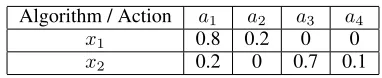
Algorithm / Action a1 a2 a3 a4
x1 0.8 0.2 0 0
[image:2.612.340.531.51.90.2]x2 0.2 0 0.7 0.1
Table 1: Algorithms’ pdfs used in our simple example.
Given a state, there is a certain probability that the algorithm outputs the true best action, and a certain probability for other actions. Letpx
a be the probability ofxselecting an actiona. Although we use the pdfs in our analysis, in general they may be unknown. Our analysis allows a deeper understanding of the conflict between learning over algorithms or actions, but a designer may still need to estimate the pdfs when taking a deci-sion between both approaches. There are examples of estimat-ing algorithms’ pdfs in the literature [Marcolinoet al., 2013; 2014; Jianget al., 2014]. Our theoretical analysis is done by comparing the likelihood of selecting the (unknown) optimal actiona∗, which maximizes the expected sum of discounted
rewards. We consider two RL agents,P1andP2, which reason over actions and algorithms, respectively.
Simple Example
Consider a single state, four actions{a1, a2, a3, a4}and two available algorithms{x1, x2}. We assumea1is the optimal action, but that is not known in advance, and the algorithms select each action according to the probabilities shown in Table 1, which results from their reasoning procedures.
In the first iteration,P1picksa1with probability0.25.P2 picksx1with probability0.5, which selectsa1with probability
0.8. Hence,P2selectsa1indirectly with probability at least
0.5·0.8 = 0.4>0.25. ThusP2’s expected performance is better thanP1’s. In the next few iterationsP2 is even more likely to pickx1, whileP1may still need to explore further, until finally playing enough training iterations for the action-value ofa1to be higher than the other actions.
When the number of training iterations becomes sufficiently large,P1learns to always selecta1, andP2to always select
x1. However, sincex1selectsa1with probability0.8, it turns out thatP2selectsa1with probability0.8<1, and hence is outperformed byP1in the long run. Therefore, until a certain number of training iterations, a RL agent may perform better by learning over algorithms, depending on the algorithms’ pdfs. In the long run, however, learning over actions will always perform better. We formalize this notion below.
3.1
Theoretical Analysis
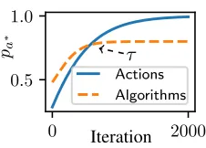
Our main result is a sufficient condition for learning over algorithms to outperform learning over actions. That allows a formal guarantee when learning over algorithms, besides guiding in the number of algorithms used, as we discuss next.
P1 or P2 selects the best choice (best actiona∗ or best algorithmx∗, respectively) with a certain probabilitypi. Let lbe the current training iteration. As usual, we consider RL agents wherel→ ∞ ⇒pi→1. We modelpiby a learning curve given by the function1−(ξi+el×βi)−1, whereξiand
0 2000 0.5
1.0
Actions Algorithms
τ
pa∗
[image:3.612.118.231.52.133.2]Iteration
Figure 1: Theoretical learning curves.
events. They converge to 1 in a diminishing returns fashion, as it would be expected in a training process. We then have:
Theorem 1. Let Pli be the probability that Pi picksa∗ at iterationl. Pl2 > P1
l for a finite number of iterations, if∃
x∈X, wherepx a∗> |
X|
|A|. Ifl→ ∞, however,P
1 l ≥ P
2 l.
Proof. IfP2selectsx∗, it indirectly selectsa∗with probability
px∗
a∗. Hence, at iteration l it selectsa∗ with probability at
least(1−(ξ2+el×β2)−1)×px
∗
a∗. P1, on the other hand,
selectsa∗ with probability 1
−(ξ1+el×β1)−1. Hence, if
px∗
a∗> 1−(ξ1+1) −1
1−(ξ2+1)−1, thenP2selectsa
∗with higher probability
thanP1in the first iteration (l= 0). Eventually, however,P1 outperformsP2, sinceliml→∞1−(ξ1+el×β1)−1= 1, and
liml→∞(1−(ξ2+el×β2)−1)×px
∗
a∗ =px ∗
a∗ ≤1. As in the first
iterationP1selects randomly,1−(ξ1+1)−1= |A1|. Similarly,
1−(ξ2+1)−1= |X1|. Therefore,ξ1=|A1|−1andξ2=|X1|−1.
Hence, if: px∗ a∗ >
1− 1 1 |A|−1+1
1− 1 1 |X|−1+1
px∗ a∗ >
1−|A|A|−1|
1−|X|−1 |X|
px∗ a∗ >
|X|
|A|,thenP2outperformsP1until a certain iterationτ. We only need onexsuch thatpx
a∗> |
X|
|A|, sincep
x∗ a∗≥pxa∗.
We show examples of P1 and P2’s theoretical learning curves in Figure 1. τ is the training iteration where learn-ing over actions starts to outperform learnlearn-ing over algorithms. Note that Theorem 1 gives us sufficient, but not necessary conditions. That is, ifpx
a∗ >|
X|
|A|, we have aformal guarantee
that learning over algorithms is better than over actions until a certain training iterationτ. However, there could be cases wherepx
a∗≤
|X|
|A|,∀x, andP2still outperformsP1.
For instance, consider 2 actions and 10 algorithms, where
px
a∗ = 0.99,∀x. Inl = 0,P1picksa∗with probability0.5, whileP2with probability0.99, even though0.99< |
X|
|A|= 5. P2outperformsP1up to a certain training iterationτ. The previous theorem shows thatτ >0if∃x, px
a∗>
|X|
|A|. We can
obtain a lower boundτ0forτ, by solving the following
equa-tion:1−(ξ1+eτ
0
×β1)−1=
1−(ξ2+eτ
0
×β2)−1
×px∗ a∗,
since the probability ofP2selectinga∗is at least(1−(ξ2+
eτ0×β2)−1)×px∗
a∗. Hence, up to training iterationτ0, we have
aformal guaranteethatP2is better thanP1, if the theorem condition is satisfied. Ifx∗is unknown, we derive a less tight
lower boundτ00 < τ0 by solving: 1
−(ξ1+eτ
00×β 1)−1 =
1−(ξ2+eτ
00×β 2)−1
×px
a∗, where x is any algorithm.
Hence, if one is able to estimatepx
a∗(for at least onex) and β, then one would also have a lower bound forτ, leading to a formal guarantee for learning over algorithms up to that training iteration (ξcan be calculated given|A|and|X|).
Additionally, note that Theorem 1does notsay that we must have one algorithm whose probability of playinga∗is higher
than the probability of playing any othera. The condition
px a∗> |
X|
|A| can be valid, even if∃a6=a
∗such thatpx a > pxa∗.
In fact, we can show that learning over algorithms outperforms over actions in a very large action space, even if the probability of an algorithm selecting the best action is very small:
Corollary 1. As|A| → ∞,P2is better thanP1for a finite number of iterations, if and only if∃x, wherepx
a∗>0.
Proof. Follows fromlim|A|→∞||XA||= 0, thusp
x
a∗ >0
satis-fies Theorem 1. The “only if” side is trivially true.
Hence, if the number of actions is very large, we only need
px
a∗>0for at least one algorithm. This result is very relevant
even in domains where a designer cannot easily estimatepx a∗.
Interestingly, however, Theorem 1 seems to suggest that the higher the number of algorithms, the worse, as we have that:
Corollary 2. If |X| = 1,xonly needs to play better than uniformly random. As|X|grows, however, the sufficient con-dition eventually is never satisfied, independent ofpx
a∗.
Proof. Follows immediately from ||XA|| → |A1| for|X| → 1,
hence we needpx
a∗> |A1|. Likewise,|
X|
|A| >1for|X|>|A|,
hence we would needpx
a∗>1, which is impossible.
In fact, if there is a fixed algorithm x, wherepx a∗ ≥px
0
a∗, ∀x0
6
=xin all states, then we should always pickx. Intuitively, however, it should be beneficial to have multiple algorithms to choose from.Informally, this may happen because different algorithms may perform better at different states, as discussed in Marcolinoet al.[2013]. That is, in many domains we do not have a fixed algorithmxthat has a higher probability of select-inga∗than the other algorithms in all states. Therefore,|X|
may implicitly also affect the probability ofP2selectinga∗, sinceP2
l ≥(1−(ξ2+el×β2)−1)×px
∗
a∗(remember thatx∗is
the algorithmxwith the highestpx
a∗across allx∈X). Hence,
informally, as the sizenofXgrows, we may have a greater chance of adding a newxnthat has a higher probability of play-inga∗than the other algorithms (i.e.,pxn
a∗ > pxa∗i,∀0≤i < n).
Therefore, although adding a new algorithm may sacrifice ini-tial performance, it may lead to a higher convergence point (i.e., a higher value forP2
l ≥(1−(ξ2+el×β2)−1)×px
∗
a∗as l→ ∞). A larger value forPl2asl → ∞also increases the number of training iterations where the curvePl2is abovePl1. That is, we may have thatτX0 > τX, if|X0|>|X|. Hence,
a larger|X|should increase the number of training iterations whereP2still outperformsP1.
Formally, however, it is not true thatτincreases with|X|
px
a∗, then we can show thatτincreases with|X|. Similarly as
before, this does not mean that an algorithm designer would directly sample a number from a distribution in order to “de-cide”px
a∗. We are just proposing to model the phenomenon of
new algorithms being created as a distribution overpx a∗. For
instance, given a set of algorithmsX0, one can calculate the av-erage and standard deviation over allpx
a∗, if one assumes that px
a∗comes from a Gaussian distribution. As|X0|grows, the
calculated average and standard deviation would approximate those of the true distribution. Hence, in order toformallystudy the effect of adding new algorithms, we evaluate different distributions forpx
a∗. We analyze three possible cases below:
(i) whenpx
a∗ comes from a uniform distribution; (ii) when px
a∗comes from a Gaussian; (iii) when there is a fixed pool
of algorithmsX˜to choose from. Similar techniques could be employed to analyze the most appropriate distribution for a given domain.
The uniform distribution could model the case where there is not yet an established framework for developing “strong” algorithms (i.e., with a highpx
a∗). Hence, the designer would
not be able to develop an algorithmxwithpx
a∗ greater than
some boundu; and given a certain state, the algorithm may be strong or weak with equal likelihood.
The Gaussian, on the other hand, models a situation with common knowledge or an established framework to develop strong algorithms (e.g., Monte Carlo Tree Search for computer Go). Then, we can expect that, in a set of algorithms, there will be a mean and a variance overpx
a∗(the variance resulting
from different design decisions or parameter configurations). Finally, we also consider the case where there is a fixed, previously known pool of algorithms available. That is, the designer must choose an algorithmx0∈X˜ to include inX.
We start by analyzing the uniform distribution:
Proposition 1. If the underlying algorithm creation process originatesxi withpax∗i ∼ U(0, u), then: (i)px
∗
a∗ grows with |X|in expectation; (ii)∃xwherepx
a∗>
|X|
|A|in expectation, if
and only if|X|< u× |A| −1
Proof. The expected value of thek-th order statistic of the uniform distribution withnsamples is given by: kn+1×u. Hence, the expected maximum value forpx
a∗when|X|=nis nn+1×u
(which grows withn). In order fornn+1×u >||XA||, we must have thatu× |A| > n+ 1 n < u× |A| −1. Conversely, if|X| = u× |A| −1 +z, forz ≥0, we would have that:
(u×|A|−1+z)×u u×|A|+z >
|X| |A|
(u×|A|−1+z)×u (u×|A|−1+z) >
u×|A|+z
|A| u× |A|> u× |A|+z, which is not possible forz≥0.
Sincepx∗
a∗grows with|X|, the proposition seems to indicate
that we should use as largeXas possible up to the upper bound
u× |A| −1. Interestingly, however, we show in synthetic experiments (Section 3.2) that performance still improves for
|X| ≥u× |A| −1.
For the Gaussian, we find that:
Proposition 2. If the underlying algorithm creation process originates algorithmsxiwithpxai∗ ∼N(µ, σ)(truncated to
the interval[0,1]), then: (i)px∗
a∗grows with|X|in expectation;
(ii)∃x, wherepx
a∗>||XA||in expectation, by following in order
of priority: (a)|X| ≥741, if|A| > µ+3σ|X| ; (b)|X| ≥44, if
|A|> µ+2σ|X| (c)|X| ≥7, if|A|>µ+σ|X|.
Proof. From the “68–95–99.7” rule, we have:p(px
a∗ ≥µ+ σ)≈ 0.5− 0.6827
2 = 0.15865;p(p x
a∗ ≥µ+ 2σ) ≈0.5−
0.9545
2 = 0.022275; p(p x
a∗ ≥ µ+ 3σ) ≈ 0.5− 0.99732 =
0.00135. Hence, in order to have in expectation at least one
xsuch thatpx
a∗≥µ+σ, we need at leasttσsamples, where
tσ×0.15865 = 1 tσ ≈7. Likewise, forpxa∗ ≥µ+ 2σ,
we need at leastt2σ ≈ 44; and forpxa∗ ≥ µ+ 3σ, at least t3σ≈741.µ+3σ≥µ+2σ≥µ+σ(the equality comes from
px
a∗>1being equivalent topxa∗= 1). Hence,px ∗
a∗grows with |X|, in expectation. Now consider the sufficient condition
px a∗ >
|X|
|A|. For p
x
a∗ ≥ µ+ 3σ in expectation, we need µ+ 3σ≥ ||XA|| |A|>
|X|
µ+3σ. Likewise, forp x
a∗≥µ+ 2σ,
we need|A|> µ+2σ|X| ; and forpx
a∗ ≥µ+σ,|A|>µ+σ|X|.
Hence, Proposition 2 allows a designer to estimate how many algorithms to use, even without an estimation ofpx
a∗
available. However, the proposition requires an estimation ofµ
andσ, which might come from previous knowledge designing and/or analyzing algorithms for the specific domain.
Fundamentally, however, even if all distribution parameters are unknown, Proposition 1 and Proposition 2 show that under distribution assumptions, one can expectpx∗
a∗to grow with|X|.
SinceP2converges to(1−(ξ2+el×β2)−1)×px
∗
a∗, thenτalso
grows with|X|. We study this further in Section 3.2. Next, we do not assume an underlying distribution. Instead, algorithms must be chosen from an existing poolX˜ (X⊆X˜):
Proposition 3. Let Pxi be the probability that xi has the
highestpx
a∗ (across allx ∈ X˜) in a states. Letpe be the expected value ofpx
a∗ inX˜. Then, in expectation: (i)px ∗
a∗
grows with|X|; (ii)∃x, wherepx a∗>|
X|
|A|, if|X|< pe× |A|.
Proof. Givennalgorithms, the probability that at least one of them has the highestpx
a∗ (across allx ∈ X˜) isp= 1− Qn
i=1(1− Pxi). Clearly,p → 1 asn → ∞, and thusp
x∗ a∗
grows with|X|. However, to satisfy the sufficient condition, we must havepe> |
X|
|A| |X|< pe× |A|.
Proposition 3 allows an estimation of the best|X|asbpe×
|A|c, givenpe. With a fixedX˜, in some domains one could estimatepe by experimentation over a set of states with a known ground truth. Fundamentally, however, it again shows that one should expectpx∗
a∗(andτ, consequently) to grow with |X|. We study this further in the next section.
3.2
Synthetic Experiments
0 1500 3000
Iteration
0 1
pa
∗
[image:5.612.127.225.52.133.2]Actions Algorithms
Figure 2: Example ofpa∗curves.
simulation, we create an agent that learns over actions, and another that learns over algorithms. For both we consideredα
andstarting as1, and decaying at the rate0.999. We sample
px
a∗ from different distributions, to simulate the creation of
algorithms in a given domain.
For each experiment, we run 1000 simulations of 10000 training iterations each. As an example, Figure 2 shows the probability of playing the best action (pa∗) when learning over
actions or algorithms, for a Gaussian model (black lines shows meanpa∗, and colored areas indicate the standard deviation).
Note how the curves follow a similar shape as the ones pre-dicted by our theory (Figure 1). In the appendix1, we show that the reward curves also follow a similar shape.
Our theoretical analysis does not yet give the exact number of iterationsτwhere learning over algorithms is better. Hence, in Figure 3 we study howτ changes as several parameters change (problem size |A|, algorithm set size |X|, uorµ), under a uniform or Gaussian model. A curve beyond the y-axis means thatτ >10000. We repeat the whole procedure 5 times, and the error bars show the confidence interval (p= 0.01). When changing one parameter we fix the others (100 actions, 25 algorithms,u= 0.5,µ= 0.4). We see thatτgrows with statistical significance, under all parameters considered, for both models. When increasinguandµwe increase the overall expected performance of the algorithms, and hence this result is expected. It is interesting to note, however, that the curves tend to grow in an exponential fashion.
Concerning|A|, the meeting pointτ also tends to grow exponentially. Hence, it gets more advantageous to learn over algorithms as problems grow in complexity. This happens since it gets harder for a RL agent to find the best action, as it requires more exploration. On the other hand, we can still seeτincreasing with|X|. That is, even though it gets harder to find the best algorithm, px∗
a∗ tends to increase with|X|,
compensating for the harder exploration, as we discussed in our analysis. Based on Theorem 1, one may expectτto drop when|X|>|A|. Interestingly, however, we see thatτtends to converge as|X|grows for both models, instead of dropping (remember that the theorem only gives sufficient conditions). Our theory focused onpa∗, but the actual reward obtained
may be more significant. We evaluated the reward and cumula-tive reward, and found similar results (shown in the appendix1). In the uniform model reward curves, however, we notice that
τstarts to drop when|X| |A|.
1
http://www.lancaster.ac.uk/staff/sorianom/ijcai18-ap.pdf
200 400 600
Problem Size (|A|) 500
1000 1500 2000
τ
0 100 200 300
Algorithm Set Size (|X|) 360
380 400 420
τ
0.3 0.5 0.7 0.9
Upper Bound (u) 200
500 1000 1500
τ
(a) Uniform Model
100 150 200 250
Problem Size (|A|)
700 1000 1500 2000
τ
0 100 200 300
Algorithm Set Size (|X|)
600 1000 1500 2000
τ
0.1 0.3 0.5
Mean (µ) 200
1000 2000 3000
τ
[image:5.612.332.538.64.303.2](b) Gaussian Model
Figure 3:τas number of actions, algorithms,uandµgrows.
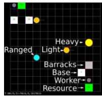
Figure 4: Screenshot ofµRTS.
4
Learning over Algorithms in RTS Games
We evaluate learning over algorithms in a real-time strategy (RTS) game, which is a very complex domain, where directly learning over actions is impractical. The number of actions for a given state is estimated as over1050 [Onta˜n´onet al., 2013]. Hence, we would need over1050training iterations just to explore a single time all the possible actions for a single state. The objective of this section, therefore, is to demonstrate that we can obtain a good performance when learning over algorithms in a complex and relevant domain.RTS games are adversarial, normally involving resource management, construction, and combat between a large num-ber of military units. They impose a great challenge for AI algorithms, since they have huge action and state spaces and require fast decisions. In this paper we useµRTS, a simplified RTS game developed for AI research2.
A screenshot of µRTS is shown in Figure 4. InµRTS, entities are eitherbuildings,unitsorresources. Buildings are eitherbases, which can produceworkersorbarracks, which
2
[image:5.612.384.485.334.430.2]produce military units. Units are eitherworkers, which harvest resources and have limited combat ability; or military units. Military units are:heavyandlight, which are strong but slow or weak but fast melee units, respectively; orranged, which are long range attack units.
A set of four simplerushalgorithms is available inµRTS: (i) Worker: create worker units, have one of them gather resources, and send all others to attack; (ii)Ranged: use a worker to gather resources. With enough resources, build a barrack and generate ranged units, sending them to attack. (iii)Heavy: same as Ranged, but creates the heavy unit instead; (iv)Light: same as before, but creates the light unit. In addition, we implemented two algorithms: (v)BuildBarracks: build a new barrack, allowing faster production of military units; and (vi) Expand: build a new base, increasing the production of worker units and faster gathering of multiple resources. All these compose our setX. In order to handle the large state space, we propose next a Function Approximation approach.
4.1
Function Approximation (FA)
In this section, we say that we are taking an “action”a∈A
in a stateseven though we are selecting an algorithmx∈X. This is to follow the traditional notation in RL literature. The main idea of FA is to learn a functional representation of the action-value functionQ. This allows us togeneralizeQfor similar state-action pairs. We use SARSA [Rummery and Niranjan, 1994], with linear function approximation. Hence, a statesis represented by a feature vector[k1(s), . . . , kn(s)], andQ(s, a)is approximated byQ˜(s, a, w) =Pn
i=1ki(s)·wi, where [w1, . . . , wn]a is a weight vector for action a. The learning problem is to find the best weights for each action. Each time the agent takes an actiona, observes the next state
s0, and chooses an actiona0ins0, we updatew
iwith: ∆wi=
α(r+γQ˜(s0, a0, w)
−Q˜(s, a, w))×ki(s), whereαis the training step size.
The features for a given state of µRTS are obtained as follows: we split the map into3×3quadrants of equal size. Within each quadrant, the number of units of each type owned by each playerpis a separate feature. Thus, 9 quadrants, 7 unit types and 2 players lead to9×7×2features. Additionally, the cumulative average health of each player’s units within each quadrant is included, leading to9×2 more features. We also include the resources harvested by each player, the current game time and the independent term, with value1. Hence, givenρp ={u11, . . . , u19, . . . , u17, . . . , u97}, whereu
j i is the number of units of typeui in quadrantj for player
p; andβp = {h11, . . . , h91, . . . , h17, . . . , h97}, whereh j i is the cumulative average health of units of typeui in quadrantj; the feature vector is:k= [1, ρ1, ρ2, β1, β2, ω1, ω2, t], where
ωp is the amount of resources owned by playerp, andtis the current game time. This linear combination of features is replicated for eachx∈X. Hence, we have|X|equations with
|k|features, leading to|X| × |k|weights to adjust. We select an algorithmx∈Xusing exponentially decaying-greedy (decayed after every training game).
4.2
Results
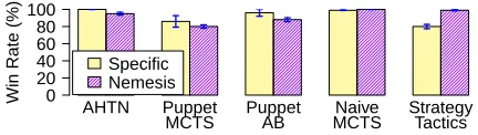
We evaluate the performance of learning over algorithms using the proposed FA approach. We compare against the state of
Win Rate (%) 200 40 60 80 100
AHTN Puppet
MCTS PuppetAB MCTSNaive StrategyTactics Specific
[image:6.612.327.543.56.117.2]Nemesis
Figure 5: Learning over algorithms against state of the art players.
the art inµRTS: AHTN, PuppetMCTS, PuppetAB, NaiveM-CTS and StrategyTactics. They are described in Section 2 and references therein. StrategyTactics won the 2017µRTS competition, and NaiveMCTS was in the top 5. We used the map “basesWorkers24×24”, and the best parametrization we found: α= 10−4,γ = 0.9,exponentially decaying from
0.2against PuppetAB, PuppetMCTS and AHTN; and decay-ing from0.1for NaiveMCTS and StrategyTactics, after every game (decay rate≈0.9984). All games have 3000 cycles at most, declared a draw on timeout. Rewards are -1, 0 or 1 for defeat, draw and victory, respectively.
We perform two evaluations. In the first, namedSpecific, we trained FA in 500 games against PuppetAB, PuppetMCTS and AHTN; and in 100 games against NaiveMCTS and Strat-egyTactics. The resulting policy is tested against the same adversary that FA was trained against. In the second, named Nemesis, we: (i) trained FA against PuppetMCTS, fixing the resulting policy; and (ii) trained a new instance of FA against the resulting policy of (i), in 500 games. The single resulting policy of (ii) is tested against all adversaries (showing robust-ness). All tests have 100 games, withα = = 0. We ran 5 repetitions of all experiments, and the error bars show the 99% confidence interval. We consider statistical significance asp≤0.01. Figure 5 shows the results.
In both cases FA significantly defeats all opponents, with win rates higher than 80%.NemesisandSpecifichave similar win rates, butNemesisis significantly better against Strate-gyTactics. We believe this happens becauseNemesisfurther elaborates on a policy that was already strong (the resulting policy of FA trained against PuppetMCTS).
Allowing algorithm switches at any state could have a neg-ative effect: it could happen so frequently that algorithms would not be able to follow a course of action. Indeed, the agent may switch “too fast” during exploration, but eventually it learns a strong policy, and tends to pick a certain algorithm repeatedly if this leads to higher performance. On the other hand, the agent learns to switch to different algorithms when that is more profitable. Figure 6 confirms both situations with theSpecific agents, by showing (a) the average number of times an algorithm is chosen consecutively and (b) the average percentage of selections (error bars indicate standard devia-tion). Hence, all algorithms tend to be chosen, but at different proportions depending on the adversary.
A vg Repetition 0
5 10 15
AHTN Puppet MCTS
Puppet AB
Naive MCTS
Strategy Tactics Light
Ranged HeavyWorker BuildBarracksExpand
(a) Repeated Selection
Ratio (%)
0 25 50 75 100
AHTN Puppet
MCTS PuppetAB MCTSNaive StrategyTactics Light
Ranged HeavyWorker BuildBarracksExpand
[image:7.612.71.276.51.210.2](b) Selection ratio
Figure 6: Average repeated selection of algorithms.
Win r
ate (%)
0 20 40 60 80 100
AHTN Puppet MCTS
Puppet AB
Naive MCTS
Strategy Tactics
Nemesis Light Ranged Heavy Worker Nemesis
Figure 7: Algorithms and FANemesisagainst all AI players.
0.004,0.61,0.04,0.14; for AHTN, PuppetMCTS, PuppetAB, NaiveMCTS and StrategyTactics, respectively. Additionally, the last set of bars shows that all algorithms are individually defeated byNemesis.
5
Conclusion
Although action abstractions have been introduced before, our model for learning over algorithms gives novel guide-lines backed by a theoretical analysis. Synthetic experiments demonstrate an increase in relative performance with action and algorithm set sizes. We also introduce a Function Approx-imation approach for learning over algorithms in RTS games, significantly outperforming state-of-the-art search-based play-ers. The source code of synthetic andµRTS experiments are available at: https://github.com/andertavares/syntheticmdps and https://github.com/SivaAnbalagan1/micrortsFA, respec-tively.
Acknowledgments
We would like to thank Fapemig, CNPq, CAPES, and the School of Computing and Communications for their support. We also thank Tom McCracken for kindly checking our code.
References
[Barrigaet al., 2015] Nicolas A. Barriga, Marius Stanescu, and Michael Buro. Puppet Search: Enhancing Scripted Behavior by Look-Ahead Search with Applications to Real-Time Strategy Games. InAIIDE, 2015.
[Barrigaet al., 2017] Nicolas A. Barriga, Marius Stanescu, and Michael Buro. Combining strategic learning and tactical search in real-time strategy games. InAIIDE, 2017.
[Barrigaet al., 2018] Nicolas A. Barriga, Marius Stanescu, and Michael Buro. Game Tree Search Based on Non-Deterministic
Action Scripts in Real-Time Strategy Games. IEEE Transactions
on Games, 10(1):67–77, 2018.
[Bontrageret al., 2016] Philip Bontrager, Ahmed Khalifa, Andr´e Mendes, and Julian Togelius. Matching Games and Algorithms for General Video Game Playing. InAIIDE, 2016.
[Churchill and Buro, 2013] David Churchill and Michael Buro. Portfolio Greedy Search and Simulation for Large-Scale Combat in StarCraft. InCIG, 2013.
[Dietterich, 2000] Thomas G. Dietterich. Hierarchical reinforce-ment learning with the MAXQ value function decomposition.
JAIR, 13:227–303, 2000.
[Jianget al., 2014] Albert Xin Jiang, Leandro Soriano Marcolino, Ariel D. Procaccia, Tuomas Sandholm, Nisarg Shah, and Milind Tambe. Diverse randomized agents vote to win. InNIPS, 2014. [Lagoudakis and Littman, 2000] Michail G. Lagoudakis and
Michael L. Littman. Algorithm selection using reinforcement learning. InICML, 2000.
[Lelis, 2017] Levi H. S. Lelis. Stratified Strategy Selection for Unit Control in Real-Time Strategy Games. InIJCAI, 2017.
[Marcolinoet al., 2013] Leandro Soriano Marcolino, Albert Xin Jiang, and Milind Tambe. Multi-agent team formation: diver-sity beats strength? InIJCAI, 2013.
[Marcolinoet al., 2014] Leandro Soriano Marcolino, Haifeng Xu, Albert Xin Jiang, Milind Tambe, and Emma Bowring. Give a hard problem to a diverse team: Exploring large action spaces. In
AAAI, 2014.
[Onta˜n´on, 2017] Santiago Onta˜n´on. Combinatorial multi-armed ban-dits for real-time strategy games.JAIR, 58, 2017.
[Onta˜n´on and Buro, 2015] Santiago Onta˜n´on and Michael Buro. Ad-versarial hierarchical-task network planning for complex real-time games. InIJCAI, 2015.
[Onta˜n´onet al., 2013] Santiago Onta˜n´on, Gabriel Synnaeve, Al-berto Uriarte, Florian Richoux, David Churchill, and Mike Preuss. A survey of real-time strategy game AI research and competition in StarCraft.IEEE Transactions on Computational Intelligence
[image:7.612.72.270.245.307.2]and AI in Games (TCIAIG), 5(4):293–311, 2013.
[Rice, 1976] John R. Rice. The algorithm selection problem.
Ad-vances in computers, 15:65–118, 1976.
[Rummery and Niranjan, 1994] Gavin A. Rummery and Mahesan Niranjan. On-line Q-learning using connectionist systems. Tech-nical report, Cambridge University, 1994.
[Saileret al., 2007] Frantisek Sailer, Michael Buro, and Marc Lanc-tot. Adversarial planning through strategy simulation. InCIG, 2007.
[Sutton and Barto, 1998] Richard S. Sutton and Andrew G. Barto.
Reinforcement learning: An introduction, volume 1. MIT press
Cambridge, 1998.
[Suttonet al., 1999] Richard S. Sutton, Doina Precup, and Satinder Singh. Between MDPs and semi-MDPs: A framework for tempo-ral abstraction in reinforcement learning.Artificial Intelligence, 112:181–211, 1999.
[Tavareset al., 2016] Anderson Tavares, Hector Azp´urua, Amanda Santos, and Luiz Chaimowicz. Rock, Paper, StarCraft: Strategy Selection in Real-Time Strategy Games. InAIIDE, 2016.
[Xuet al., 2008] Lin Xu, Frank Hutter, Holger H. Hoos, and Kevin