Engineering Design for a Horticultural
Grow–Cell Prototype
Ioannis Tsitsimpelis
MSc Mechatronics EngineeringA thesis submitted in partial fulfilment for the degree of Doctor of Philosophy
Engineering Department
This thesis is concerned with controlled environment horticulture, with a particular focus on two practical examples, namely a laboratory scale forced ventilation chamber and a full-sized prototype grow-cell developed in collaboration with an industry partner. The grow-cell belongs to a relatively new category of plant factory in the horticultural industry, for which the motivation is the maximization of production and the minimization of energy consumption. Significantly, the plants are grown under artificial lights and there is recycling of water.
The thesis is organized into two main parts. Part A of the thesis takes a systems design approach to identify the engineering requirements of the new grow-cell facility, with the prototype based on a 12 m × 2.4 m× 2.5 m shipping container. Research contributions are made in respect to: (i) the design of a novel conveyor-irrigation system for mechanical movement of plants; (ii) tuning of the artificial light intensity; and (iii) investigations into the environmental conditions inside the grow-cell. In particular, the conveyor-irrigation and lighting systems are optimized by the present author to make the proposed grow–cell more effective and sustainable. In future research, the prototype unit thus developed can be used to investigate production rates, plant quality and whole system operating costs. Nonetheless, preliminary growth trials reported within the thesis, demonstrate that Begonias semperflorens and Impatiens divine can be harvested to the satisfaction of a commercial grower.
the partitioning of indoor environment into a number of zones that have a relatively uniform thermal behaviour. The quantitative data-driven approach proposed here, first characterizes the system dynamics using measured data and, secondly, exploits Agglomerative Hierarchical Clustering (AHC) and k-means clustering to determine the thermal zones. The practical utility of the new approach is evaluated using the laboratory example i.e. a 2 m × 1 m × 2 m chamber with two axial fans, a heating element, and an array of thermocouples. In this case, the modelling approach yields Hammerstein type models which are subsequently used for both single and multi–zone control system design. The laboratory facility was used for this research since it was readily available for these closed-loop control experiments.
I declare that this Thesis is my own work, and has not been submitted in substantially the same form for the award of a higher degree elsewhere.
Acknowledgements
The first person I want to thank for this experience is my mentor, Professor C. James Taylor. His guidance, support, and positive spirit were invaluable and catalytic to my academic progress. I can never thank him enough.
I would also like to thank the Centre for Global Eco-Innovation and the industrial partner, NP Structures, for funding this project.
To my mother Sappho, grandmother Ioanna, brother George, and cousin Costas.
Contents
1 Introduction 1
1.1 Motivation and aims . . . 2
1.2 Micro-climate modelling . . . 4
1.3 Research objectives . . . 5
1.4 Articles arising . . . 6
1.5 Thesis organisation . . . 7
2 Introduction to Part A 9 2.1 Protected environment crop growth . . . 10
2.2 Engineering requirements . . . 14
2.3 Artificial Lighting . . . 15
2.4 Mechanical Movement of Plants . . . 17
2.5 Thermal Stratification . . . 18
2.6 Research Objectives. . . 19
3 Development of Grow-cell Prototype 22 3.1 Container and Air-conditioning unit . . . 22
3.2 Conveyor System . . . 23
3.3 Irrigation System . . . 26
3.4 Lighting . . . 26
3.5 Instrumentation . . . 27
3.6 LED Characterisation & Optimisation . . . 28
3.6.1 Preliminary LED Growth Test . . . 32
3.7 Conveyor-Irrigation System Tuning . . . 33
3.9 Conclusions . . . 38
4 Growth Trials 39 4.1 January-March 2015 Growth Trial . . . 39
4.2 June-July 2015 Growth Trial . . . 42
4.3 Temperature and humidity observations . . . 42
4.4 Conclusions . . . 47
5 Discussion and Conclusions 50 5.1 Freight container and air-conditioning unit . . . 50
5.2 Conveyor system . . . 51
5.3 Irrigation system . . . 52
5.4 Lighting system . . . 53
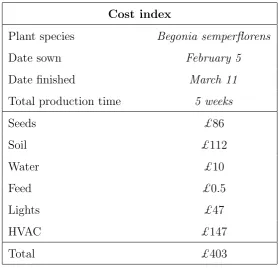
5.5 Growth trials cost and energy usage . . . 54
5.6 Commercial grow-cell concept revisited . . . 56
5.7 Conclusions . . . 57
6 Introduction to Part B 60 6.1 Multi-zone models . . . 61
6.2 Laboratory scale forced ventilation chamber . . . 63
6.3 Motivational example . . . 65
6.4 Research Objectives. . . 67
7 Cluster Analysis 71 7.1 Clustering Algorithms . . . 72
7.1.1 AHC algorithm . . . 72
7.1.2 K-means algorithm . . . 74
7.2 Data collection . . . 75
7.3 Data processing . . . 75
7.3.1 Selection of clustering variables . . . 77
7.3.2 Selection of distance metric . . . 78
7.3.3 Metaclustering . . . 78
7.4 Transfer function models . . . 79
7.5.1 Low ventilation rate . . . 82
7.5.2 Medium ventilation rate . . . 84
7.5.3 High ventilation rate . . . 86
7.5.4 Non-linear datasets . . . 89
7.6 Discussion . . . 90
7.7 Conclusions . . . 92
8 Thermal Modelling 93 8.1 Identification of temperature steady state behaviour . . . 95
8.2 Dynamic model . . . 98
8.3 Combined Model . . . 99
8.4 Preliminary evaluation . . . 100
8.5 2-dimensional Hammerstein model. . . 103
8.6 State-Dependent-Parameter extension of the 2-dimensional Hammer-stein model . . . 107
8.7 Non-linear multi-zone thermal model . . . 112
8.8 Conclusions . . . 115
9 Temperature Control Examples 118 9.1 Single thermal zone control design . . . 119
9.2 Evaluation using the non-linear model . . . 121
9.3 Experimental results . . . 125
9.4 Multiple-Input-Multiple-Output Control . . . 126
9.5 Evaluation . . . 130
9.6 Conclusions to Part B of the thesis . . . 132
10 Overall Conclusions and Future Research 136 10.1 Summary . . . 136
10.2 Future Research . . . 139
References 160 A Conveyor System Programming 161 A.1 Hardware . . . 161
A.2.1 Sweep transfer. . . 163
A.2.2 Horizontal transfer . . . 164
A.2.3 Fault detection circuitry . . . 165
A.2.4 Communication with the HMI . . . 165
A.2.5 Control panel, hardware schematics, and code . . . 165
B LED lights selection 170
C Grow-Cell Subsystem Design Guidelines 173
List of Figures
1.1 General grow-cell concept: a closed-environment mobile system, fully
occupied with plants, which are grown under artificial light in a
multi-tier configuration. The figure shows how multiple units can be stacked.
However, the research in this thesis is based on one unit, namely a
modified shipping container. . . 2
2.1 Grow-cell prototype drawing showing the basic layout of the modified
freight container (12 m × 2.4 m ×2.5 m). . . 16
2.2 Fodder barn layout with numbered sensor locations. . . 19
2.3 Daily temperature and humidity data in the south-east (i, iii) and
north-west (ii, iv) areas of the fodder barn. The blue, red and yellow
traces correspond to the top, middle and bottom layers of each area.. 20
3.1 Conveyor and racking design schematic diagram. . . 23
3.2 Conveyor structure detail showing (i) skate wheels attached to the
main circuit, (ii) grooved circuit to keep the body frame vertical, (iii)
sweep motion motor and (iv) horizontal motion motor. . . 24
3.3 Conveyor structure operation for anti–clockwise rotation (i) system
ready for sweeping hangers, (ii) during sweep motion and (iii) system
ready for horizontal motion. . . 25
3.4 LED lights and empty plant growth trays. . . 27
3.5 Sensor locations in the grow–cell. Note that sensor 31 (not shown) is
located at the air intake of the unit. . . 28
3.6 Spectral output of lights installed in the grow–cell. . . 29
3.7 Schematic diagram of the 0.9 m× 0.5 m board for measuring PPFD
3.8 Spatial distribution of light intensity (µmols m s ) at a distance of
20 cm. Subplots i through to vi are for voltage levels of 40%, 46.5%,
53%, 60%, 67% and 100% intensity of the variable power supply. Each
subplot indicates the light intensity over the 50 cm (vertical axis) by
30 cm (horizontal) light panel. . . 31
3.9 Single panel light intensity plotted against supply voltage expressed as a percentage of the maximum, highlighting the most energy efficient intensities (shaded).. . . 31
3.10 Spatial distribution of light intensity (µmols m−2 s−1) for 20 light panels in one layer, with i) 60%, ii) 67% and iii) 100% of the maximum power supply. Each subplot indicates the light intensity over 50 cm (vertical axis) by 6 m (horizontal). . . 32
3.11 Four weeks old Tuberous begonia plants grown under white LEDs (middle tray) and in a greenhouse (the other trays). . . 33
3.12 Steady state temperature distribution with lights switched on (upper subplot) and off (lower). Spline interpolation from the 30 point measurements using Matlab. . . 35
3.13 Steady state temperature distribution for setpoints 20◦C (i), 18◦C (ii), 16 ◦C (iii) and 14 ◦C (iv). The height and length axis (not shown) for each subplot are identical to those in Fig. 3.12.. . . 36
3.14 Supply and exhaust (dashed trace) temperature associated with Fig. 3.13. 36 3.15 Transient response of temperature distribution in the growing area shown at 10 minute intervals from the moment the lights are switched on (i) through to 1.5 hours later (x). The height axis, length axis and legend (not shown) for each subplot are identical to those in Fig. 3.12. Numerical values are illustrative temperature point measurements,◦C. 37 4.1 Begonia semperflorens plants germination period. . . 40
4.2 Three week old Begonia semperflorens plants. . . 41
4.3 Finished Begonia semperflorens plants before harvest. . . 41
4.4 Finished Impatiens divine before harvest. . . 43
4.5 Finished Begonia semperflorens before harvest. . . 43
4.7 Root growth of Begonia semperflorens. . . 44
4.8 UnfinishedBegonia tuberhybrida. . . 45
4.9 Selected temperature sensor readings from layer 2 during the first
trial, January 30 to February 10. The numbers 2, 7, 12, 17, 22 and 27
refer to the sensor locations in Fig. 3.5. . . 46
4.10 Interpolated temperature spatial distribution during lighting (upper
plot) and dark (lower) hours, January 30 to February 10. . . 47
4.11 Interpolated humidity spatial distribution during lighting (upper plot)
and dark (lower) hours, January 30 to February 10. . . 48
4.12 Temperature and humidity responses throughout the five week period
of the second trial, plotted against sample number (3 hour samples).
The set-points, active and empty layers are indicated by blue, red and
black coloured traces respectively. . . 48
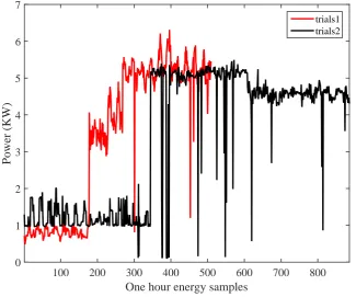
5.1 Instantaneous power used by the HVAC unit throughout both trials,
with red and black traces depicting the first and second trials respectively. 57
6.1 Layout of the sensor locations within the test chamber. . . 64
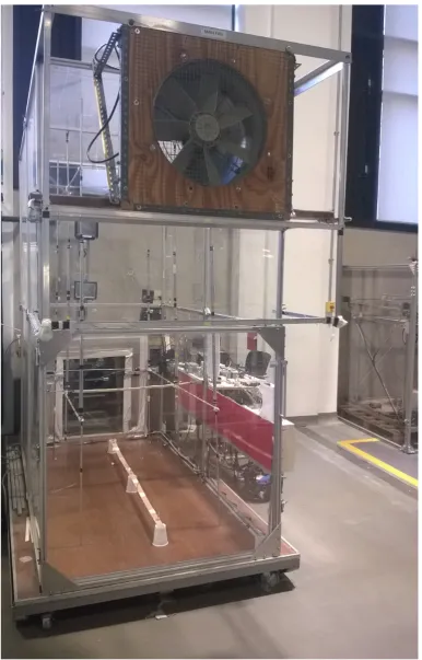
6.2 Laboratory forced ventilation test chamber [Leigh, 2003, Tsitsimpelis,
2012]. . . 66
6.3 Open–loop experiment showing the fan and heater inputs (middle and
bottom subplots), together with the temperature from each
thermo-couple (upper subplot). . . 68
6.4 Resemblance between each thermocouple and an illustrative reference
thermocouple, for the experiment in Fig. 6.3, with zone 1 highlighted
in bold. The reference thermocouple has in this case a value of zero. . 68
7.1 Typical responses for a step change in the heater input experiment.
The upper plot depicts data that have been collected for a low fan
setting and a high heater setting, whereas the bottom plot shows the
same for a high fan setting and a low step change in the heater input. 76
7.2 Two data-sets that have either the fan (ventilation rate) or the heater
7.3 Model representation on one of the two zones that were derived by
visual inspection of the data presented in section 6.3. The thick trace
(equation 7.6) represents the model fit to the average zone data. . . . 80
7.4 Three-dimensional plot that shows the structure of the data when
plotted against 25%, 50%, and 90% average sample instances. Note
that although the fourth clustering variable is used for clustering, it
is simply omitted here for the sake of producing a meaningful graph.
The two clusters are depicted in triangle and square shaped points. . 83
7.5 The structure of the partitioned data when plotted as standardized
time constants (tc) against steady state gains (ssg). Similar to Fig. 7.4,
the two clusters are depicted in triangle and square shaped points. . . 83
7.6 Temperature responses of heat step experiment f15h15, colour coded
here, with the black trace representing the bottom layer temperature
locations. . . 84
7.7 Structure of data for clustering based on the raw data instances of
f15h45. . . 85
7.8 Two-dimensional structure of data for f15h45. . . 85
7.9 Silhouette plot for a clustering solution k=2, regarding f15h45. The
high values suggest a good within cluster compactness and between
cluster separation.. . . 86
7.10 Clustered data structure forf25h25, which still shows elongated but
compact enough to consider uniformity instead of the two zones shown
here by triangular and square points. Note that the gradient is less
than 2◦ C at all sampled instances. . . 87
7.11 The top plot shows the data structure of f25h35, with location no.12
depicted here as a star symbol belonging marginally to both groups.
However, the silhouette plots suggest that it belongs to neither for a
cluster solution of k=2 . . . 87
7.12 f45h45 temperatures partitioned with respect to k-means (raw data).
The first zone (red traces) contains the front end locations (1-4),
together with the six locations of the bottom layer (5-6,11-12, and
7.13 Silhouette plots produced by using the four different clustering
ap-proaches for the f45h45 dataset. . . 89
7.14 Colour coded cluster solutionk=2. It can be seen that two types of
behaviours are indeed present within the main grid, and that they are
also meaningful; that is, they correspond in this case to the bottom
layer (red traces) and the two other layers. . . 90
7.15 Two clusters again describing the temperature distribution. This
solution confirms that for medium ventilation rate the test chamber
is partitioned in a front to back manner within the main grid. . . 90
7.16 Two clusters describing the temperature distribution for a fixed heat
setting and the fan varying. . . 91
8.1 Exemplary Hammerstein Model . . . 95
8.2 Steady state behaviour ventilation rate, with circles representing
the data, and the red trace representing the model fit solved by
equation (8.1).. . . 96
8.3 Steady state behaviour of exemplary temperature location no. 1 for
six different fan settings. The points in this figure are the steady state
temperatures derived from the experiments, whilst the solid traces
result from solving equation 8.2. . . 97
8.4 Open-loop experimental data and dynamic model for temperature,
with time-invariant fan input of 2.5V. Upper subplot: temperature
elevation (points) and linear model response (solid). Lower subplot:
heater input. . . 99
8.5 Open-loop evaluation experiment comparing the non-linear thermal
model (solid trace) with experimental data (points). The lower plot on
the left shows the predicted (effective input) steady state temperature,
while the lower right shows the fan (blue trace) and heater input
8.6 Open-loop evaluation experiment comparing the non-linear thermal
model (solid trace) with experimental data (points). Here, both input
signals are varied around their operating range. The lower plot on the
left shows the predicted (effective input) steady state temperature,
while the lower right shows the fan (blue trace) and heater input
sequences. . . 102
8.7 Schematic diagram of the 2-dimensional Hammerstein model. . . 104
8.8 Logistic growth function coefficients (clockwise from top left) x0,
ytmax,θ andcestimated from steady state temperature data collected
at different ventilation rates (points), together with second order
polynomial fit. The latter order was selected as it broadly yields
curves that follow the trend observed from the measured data . . . . 105
8.9 Evaluation of 2-dimensional Hammerstein model for the same dataset
as in Fig. 8.6. . . 106
8.10 Evaluation of 2-dimensional Hammerstein model for a dataset where
the heater shifts between 0, 50 and 100% and the ventilation rate is
varied between medium and high levels. . . 106
8.11 Evaluation of 2-dimensional Hammerstein model for a dataset where
the fan input is varied to arbitrary levels every 10 minutes, and the
heater input also changing every 15 minutes . . . 107
8.12 Second order parameter values against increasing ventilation rate;
black trace corresponds to a fixed heat setting of 1.5 V, while red,
green and blue traces correspond to fixed heat settings of 2.5, 3.5
and 4.5 V respectively. The thick blue trace depicts the heat setting
average parameter values. . . 109
8.13 Second order polynomial functions explaining each average parameter
of the sdp-model against ventilation rate. . . 110
8.14 Pole-zero maps depicted for the whole operating range. The poles are
depicted by cross marks. Each subplot shows the poles and zeros for
six different fan settings under a fixed heat setting. . . 110
8.16 Evaluation of 2-dimensional sdp Hammerstein model for the three
datasets previously utilised for evaluation. The top plot relates to
Fig. 8.9, the middle relates to Fig. 8.10, and bottom plot to Fig. 8.11. 111
8.17 Schematic diagram of illustrative two-zone thermal model. . . 112
8.18 Temperature (elevation above ambient) distribution for f15h35.
Mea-surements from all the thermocouples in the main grid are overlaid
here. . . 113
8.19 Upper subplots: (i) average temperature in zone 1 (noisy data) and
model response (smooth), and (ii) heater input. Lower subplots:
(iii) average temperature in zone 2 (noisy data) and model response
(smooth), and (iv) zone 1 temperature used as the input. . . 114
8.20 Input and output signals for evaluation experiment showing (i) fan
input, (ii) temperatures, (iii) heater input and (iv) ventilation rate. . 115
8.21 Evaluation experiment based on the proposed clustering approach,
showing zone 1 (upper subplot) and zone 2 (lower). . . 116
8.22 Evaluation experiment with user selected zones based only on the
location of the sensors, showing zone 1 (upper subplot) and zone 2
(lower).. . . 116
9.1 Proportional–Integral–Plus (PIP) control block diagram. . . 121
9.2 PIP controller implemented on a 2-dimensional Hammerstein model.. 122
9.3 PIP control simulation on the non-linear thermal model. The upper
plot shows the command input and temperature response with a black
and a red trace, respectively. The lower plot depicts the control input
with a red trace, whilst the fan and heater signals that eventually
formulate the command input are represented by dashed blue and
9.4 PIP control simulation on the non-linear thermal model. In this case,
it is the fan that induces a change in the command input. The upper
plot shows the command input and temperature response with a black
and a red trace, respectively. The lower plot depicts the control input
with a red trace, whilst the fan and heater signals that eventually
formulate the command input are represented by dashed blue and
green traces, respectively.. . . 124
9.5 PIP control simulation on the non-linear thermal model (dashed red
trace), compared with the PIP control simulation on the linear model,
for three different set-point change scenarios. . . 125
9.6 Middle-upper layer average temperature response (black dots), model
fit (red trace), and residual errors (blue trace). . . 126
9.7 Proportional-Integral-Plus zone control simulation vs data. red trace:
zone individual responses, dashed and dash-dotted black and green
traces, are the system’s and model’s average zone temperatures and
control inputs, respectively. . . 127
9.8 The upper plot shows the temperature response and model fit to a
heat step, and the lower plot shows the same for a fan step. In both
plots the dashed blue trace represents the fan setting and the dashed
red trace represents the heat setting. . . 128
9.9 Temperature difference data and model fits between zone 1 and zone
2 for a heat step (upper plot) and a fan step. . . 128
9.10 Simulation of MIMO controller with controller broadly achieving the
setpoints. The lower plot shows the control inputs i.e. uheat with a
red trace, and uf an with a blue trace . . . 131
9.11 Second exemplary simulation of MIMO controller . . . 132
9.12 Mimo control experiment with limited control action achieving the
desired temperature and temperature difference . . . 133
A.1 Control panel initial version, designed and hard-wired by the author. 166
A.3 Input hardware schematic as designed by the author. Note that in
this version, the reflective sensor that controls the starting position is
not included as it was added later on. . . 167
A.4 Main movement functions. . . 168
A.5 Alarm monitors and HMI communication. . . 169
B.1 Spectral output of each unit. Upper plot: Ghel, Illumitex (dashed trace), Jing (red trace). Lower plot: Valoya, Solidlite (dashed trace). In both plots the relative quantum efficiency curve of plants is depicted in blue colour. . . 171
B.2 PPFD distribution at 20 cm above a 90 cm×50 cm measuring board. Top plot: Ghel. Middle plot: Illumitex. Bottom plot: Jing. . . 172
B.3 PPFD distribution at 20 cm above a 90 cm×50 cm measuring board. Top plot: Solidlite. Bottom plot: Valoya . . . 172
C.1 HVAC System Design. . . 174
C.2 Power Supply System Design. . . 175
C.3 Shelving, Conveyor and Irrigation System Design. . . 176
C.4 LED Lights System Design. . . 177
D.1 Procured container . . . 179
D.2 The author hardwiring LED lights and connecting the conveyor’s motors to the power supply. The chassis of the tray carriers can also be seen. . . 180
D.3 On the top, one may see the pegs of the slotted lever mechanism that pushes the tray carriers. These are mounted on the horizontal movement rods. . . 181
D.4 The variable power supplies that were utilised the change vary the light output of the LED lights.. . . 181
D.6 At the top, one may see the sweep motor and its pushing arm sitting
below its proximity sensor, which is also its initial position.
Further-more, on the top left and right one may see the photoelectric sensors
that were utilised in the conveyor control logic. . . 183
D.7 The control and power supply room before one enters the growing area.
In this picture one may see the control panel that the author made
for the conveyor system. Above it there is the main power supply
panel. At the bottom and at the right lies the irrigation system that
was installed by the partner company, before the author modified it
List of Tables
3.1 Minimum and maximum light intensity for Fig. 3.8. . . 30
5.1 Growth trial information and cost list. . . 55
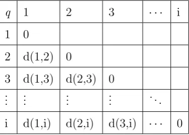
7.1 Information matrix, where q = 1,2, ..., i refers to the location of
each temperature sensor and p= 1,2, ..., j contains the values of the
associated variables . . . 73
7.2 Distance matrix that contains the pairwise difference between all
temperature locations. . . 73
8.1 Equation (8.2) optimised coefficients for each of the six power curves
displayed in Fig. 8.3, with the first and last rows relating to the lowest
and highest fan settings respectively. . . 98
8.2 Polynomial coefficients that predict the values of ytmaxu˜f an, θu˜f an,
x0u˜f an, and cu˜f an for different ventilation rate settings . . . 104
8.3 Comparison table of fitting data-sets, using the 1-dimensional,
2-dimensional, and SDP extension Hammerstein model. The type
implies which input was varying throughout a dataset. Red colour
Chapter 1
Introduction
This thesis is concerned with controlled environment horticulture, with a particular focus on the monitoring, modelling and control of environmental variables, such as temperature and humidity. The research behind the thesis consists of two separate although complementary activities, both lead by the author within the framework of a Centre for Global Eco-innovation graduate research project1. Part A of the
thesis reports on the development, optimisation and testing of a closed–environment prototype grow–cell. As illustrated in Fig. 1.1, this belongs to a relatively new category of plant factory in the horticultural industry, for which the motivation is the maximization of production and the minimization of energy consumption.
Part B of the thesis develops a novel approach for the modelling and control of the environment inside buildings more generally, particularly in relation to the statistical identification of spatial zones with similar thermal characteristics. Although motivated by measurements from the grow-cell, the new approach is developed and evaluated using a more readily available, laboratory forced ventilation test chamber. The present Chapter 1 briefly introduces the overall aims and motivation for the work, and the structure of the thesis. However, more detailed research objectives and literature reviews are provided in the opening chapter to each part of the thesis i.e. Chapter 2 (Part A) and Chapter 6 (Part B).
1The project is supported by the Centre for Global Eco-innovation (Lancaster University) and
part financed by the North West UK operational programme for European Regional Development
Funds. The industrial partner, NP Structures Limited, specialises in the design and manufacture of
Figure 1.1: General grow-cell concept: a closed-environment mobile system, fully occupied with plants, which are grown under artificial light in a multi-tier configura-tion. The figure shows how multiple units can be stacked. However, the research in this thesis is based on one unit, namely a modified shipping container.
1.1
Motivation and aims
Controlled environment horticulture is a subject nested within the wider agenda of optimising the food system, in order to deal with forthcoming changes in population and climate [FAO,2002,2015]. Today’s established protected crop growth medium is the glasshouse (and related plastic covered systems), globally occupying an estimated 8000 km2, in which intensive use of pesticides and excess water supply generally takes
place [Wainwright et al.,2014]. Hence, there is a considerable effort by stakeholders in the agricultural industry to optimize a range of sub-processes, with the aim to decrease harmful residues and energy inputs.
Such research includes investigations into the physical structure in which plants are grown, and the exploitation of modern technological know-how in order to deploy a higher level of system automation. For instance, significant work has been carried out by the industry to realize what are typically known as plant factories. These are multi-layer growing systems installed in thermally insulated, fixed or mobile buildings, and equipped with artificial light [GreenTech,2016, FreightFarms, 2016,Markham,
approach are: the flexibility to grow crops at any geographical location regardless of the external climatic conditions, reduced pesticide use and the decrease of food miles, all of which induce savings in terms of transportation costs, greenhouse gas (GHG) emissions and crop nutritional and economic value. Furthermore, by incorporating a multi-tier (vertical farming) arrangement, as in Fig. 1.1, there is the potential to significantly reduce the land area currently occupied by greenhouses. Finally, there is scope for investigation of various biological and horticultural issues, for example crop delivery date and flavour, by on–line regulation of the lights, micro-climatic and feed systems.
Plant production by means of artificial climate and artificial or hybrid light dates back to the first quarter of the 20th century. Initially, the primary motivation was to facilitate research into plant responses for different environmental conditions, with illustrative early citations including Harvey [1922],Popp [1926], Davis and R. [1928]. However, thanks to recent technological advances relating to the performance and operating costs of light emitting diode (LED) lights, it is now possible to realize such facilities for industrial use, with the long term expectation being to outpace the use of greenhouses in terms of production and energy efficiency.
A number of systems have been brought into the industrial domain over the past few years, particularly in Japan and the USA (see e.g. GreenTech [2016],
FreightFarms [2016],Markham[2014]), and interest is expected to further increase as big corporations are investing in the erection of indoor farms [Hughes, 2015,Payne,
2014]. Nevertheless, there are numerous on-going research challenges relating to their design and operation. For example, their energy requirements, air movement, dehumidification, internal racking design, different ways to deploy artificial LED lighting, and the monitoring of crop reaction to these.
the grow-cell, including temperature and humidity.
1.2
Micro-climate modelling
Ventilation rate and heat are significant inputs in the control of micro-climate surrounding plants within agricultural buildings, and the lack of effective regulation of these is a major cause of production losses. Heating and ventilation systems employed in many buildings presently deal with environmental variables in an averaging manner, utilising measurements from single locations and assuming these represent the micro-climate of the whole area. Hence, multi-zone models often approximate the problem by considering an entire room or floor as one thermal zone [Liao and Dexter, 2004, De Persis et al., 2008, Mossolly et al., 2009, Goyal and Barooah, 2012]. This is particularly true for agricultural buildings such as glasshouses (e.g. Taylor et al. [2004b]). Dealing with such micro-climatic gradients in agricultural buildings generally leads to higher costs and energy losses e.g. as staff have to physically move plants around [Kittas et al., 2003, Teitel et al.,2010]. However, the importance of manipulating environmental variables in an energy efficient manner, whilst taking account of the gradients that arise, is also clear for many other types of indoor environment (e.g.Van Brecht et al. [2003],Brande [2006],
Chen [2009]).
Multi-zone models are commonly based on physically defined locations in the facility, for which relatively homogeneous environmental conditions are assumed, say the inlet, outlet and different rooms of a building.Bleil De Souza and Alsaadani[2012] discuss some common strategies for thermal zoning, focusing on the human-built environment. However, in some practical situations, different thermal zones with similar characteristics emerge in an open space (one room) that will not necessarily be obvious from the physical layout. This is evident for the horticultural grow-cell and laboratory ventilation chamber considered in the present thesis.
avoiding undue reliance on prior hypotheses and ensuring that the resulting models are identifiable from the available environmental data. However, the identified model is only considered fully acceptable if it is also capable of interpretation in a physically meaningful manner. This represents a novel example of the data-based mechanistic (DBM) concept (see e.g. Price et al.[1999], Young [2011,2013]).
1.3
Research objectives
Although more details are provided in chapters 2 and 6, the overall objectives of the research can be briefly summarised as follows:
• To identify the engineering requirements of a new grow-cell facility, and to support the industry partner in the conversion of the shipping container procured for this purpose.
• To optimise the conveyor-irrigation system in advance of the plant growth trials. The conveyor allows for operator access to the plants and potentially provides for the automatic insertion, inspection and harvest of crops. It also ensures a more equal treatment of plants in terms of environmental variables, and adds to the circulating effect provided by the fans.
• To adapt the commercial LED units so that they are capable of varying the output light intensity; to investigate their spectral characteristics; and to use these results to optimise the balance between light intensity and energy consumption.
• To utilise statistical tools for data-driven identification of thermal zones in a building, and to use these to develop both single-zone and multi-zone control systems for temperature. Because of limitations in the existing grow-cell air conditioning unit, these new algorithmic developments are evaluated using a laboratory forced ventilation chamber.
recommendations for future developments in the grow-cell air conditioning unit, and for further research into the grow-cell concept more generally.
1.4
Articles arising
The following peer reviewed articles have arisen as a result of the research in this thesis:
• Tsitsimpelis, I. and Taylor, C. J., Micro-Climate Control in a Grow-Cell: Sys-tem Development and Overview, 19th IFAC Triennal World Congress, Cape Town, South Africa, 2014. (Conference article with preliminary design consid-erations from Chapters 2-3 of the thesis).
• Tsitsimpelis, I., Wolfenden, I. and Taylor, C. J., Development of a grow-cell test facility for research into sustainable controlled-environment agriculture, Biosystems Engineering, vol. 150, pp. 40–53, 2016. (Journal article based on Chapters 2-5 of the thesis).
• Tsitsimpelis, I. and Taylor, C. J., Partitioning of indoor airspace for multi-zone thermal modelling using hierarchical cluster analysis, European Control Conference, Linz, Austria, 2015. (Conference article with preliminary results relating to the clustering analysis in Chapter 7).
• Tsitsimpelis, I. and Taylor, C. J., A 2-Dimensional Hammerstein model for Heating and Ventilation Control of Conceptual Thermal Zones, 10th UKACC Control Conference, Loughborough, UK, 2014. (Conference article with pre-liminary results relating to the Hammerstein thermal models in Chapter 8).
The following article is in preparation for submission to a suitable journal:
1.5
Thesis organisation
The following Chapter 2 introduces Part A of the thesis i.e. concerning the devel-opment of the grow-cell prototype. Chapter 3 discusses each grow-cell subsystem in turn, followed by their preliminary testing and optimisation. This includes: the design and implementation of the conveyor-irrigation system; the tests, selection, and modification of the lighting system; and an investigation into the micro-climate that dominates the growing area. Chapter 4 presents the results of the two growth trials, held in February 2015 and June 2015. Chapter 5 concludes the first part of the thesis with a discussion of the lessons learnt, the energy use and costs derived from the growth trials, and suggestions for future development.
Part A
Development of Grow-Cell
Chapter 2
Introduction to Part A
The present Chapter 2 introduces Part A of the thesis, which is concerned with the development of a grow-cell prototype. There is significant research effort globally towards maximising the production capacity of closed growing systems, to minimise energy inputs and to minimise the use of pesticides. Many studies have shifted their research focus towards the development of plant factories and a number of tangible examples have been developed by industry. These demonstrate current technology and show that industry has the capacity to put together such structures [Markham,
2014, Payne, 2014, FreightFarms,2016, GreenTech,2016, Hughes, 2015]. However, research being conducted around the world also highlights that a wide optimisation margin, beyond the minimum necessary to just grow plants, has yet to be reached i.e. there is considerable scope for improvements in regard to production costs, energy consumption and so on [Hendrawan et al., 2014, Despommier, 2009, Kozai et al.,2015,Oguntoyinbo et al., 2015, Ohara et al.,2015, Park and Nakamura,2015,
Sugano, 2015].
large range of medium and small edible crops: a) they are not affected by external climatic conditions; instead a dedicated micro-climate is applied, which makes a crop growth task simpler and more predictable to control; b) they require negligible use of pesticides because their isolated environment inevitably reduces the number of potential infecting agents; and c) in an optimised setting, water usage can be minimised by recycling irrigated water, and by environmental controllers recycling water vapour and regulating this to minimize the frequency of the required irrigation cycles. However, in order to make such facilities viable, significant multidisciplinary research is still required.
Section 2.1 reviews the protected environment crop growth literature from its early days. Sections 2.2 through to 2.5 consider more specialist work in relation to two key topics of interest, namely (i) the options for artificial light and (ii) issues arising in relation to the mechanical movement of plants. This information is used to identify the system requirements of the prototype, representing an early research contribution of this thesis. As a result of these requirements, section 2.6 summarises the research objectives for the following chapters 3–5 of the thesis.
2.1
Protected environment crop growth
Future food supply and optimization of agriculture was already a concern by the early 20th century. Ball [1921], for example, observed that smart land manipulation by merging know–how from various scientific fields would compensate for the rapid increase of population and the lack of remaining lands suitable for cultivation. At the research end, the driver for erecting closed growing apparatuses was the inconsistent results between similar growth studies [Davis and R.,1928, Arthur et al., 1930]. At the time, this type of structure was not regarded to be commercial, but a research tool which would allow studies in plant physiology to be standardized. These are now known as growth chambers, which are in essence small scale versions of plant factories, except they are used for research purposes.
sufficient sunlight during winter months. Light was provided by 200 and 1000 W nitrogen-filled tungsten lamps, while the apparatus accounted for spatial variability by incorporating phonograph motors to rotate the plant pots [Harvey, 1922]. The sequel of that study, which was published two years later [Hendricks and Harvey,
1924], addressed the rate of growth under continuous lighting, where more than forty plant species were grown and classified in terms of light intensity and temperature needs.
Tottingham[1926] assessed temperature effects in protein content, dry matter, and sugar content of wheat, in culture chambers facilitated within a greenhouse. Wheat was grown in water, sand and soil, and means of illumination was provided both artificially and by the use of daylight. Mazda lights were used, starting from 500 W and reaching up to 2500 W for different growth trials. Two years later,
Davis and R. [1928] presented an environment chamber in which wheat was grown hydroponically. Their results demonstrated the possibility to obtain better growth than that emerging in nature, as well as the feasibility of reproducing similar growth results. The greenhouse presented by Arthur et al. [1930] featured supplementary artificial light from incandescent sources mounted on retractable rails, and the use of mixing fans for air circulation. It was further equipped with isolated rooms, which comprised gas-filled tungsten lamps put before water-glass in order to filter out infra-red radiation. Brown [1939] presented three growth chambers installed inside a greenhouse. Each one had separate soil and air temperature control systems. The chamber boundaries were made of glass in order to receive sunlight, while the air would be heated or cooled when leaving the chamber, depending on the control set-point; and diverted in turn back to the chamber through another duct. In his review paper, Parker [1946] reports on several other similar studies that were held during those years.
temperature generated in separate small chambers through air ducts. Air velocity was usually measured by “Tycos” anemometers. Carbon dioxide was also monitored and supplied by steel cylinders. Moreover, ways of measuring light intensity included iron-nickel thermocouples in the circuit with galvanometers, Macbeth illuminome-ters, Sharp-Miller photometers and pyrheliometers; while wavelength was commonly measured using quartz spectrographs.
years, covering aspects of tomato growth [Went, 1944a,b, 1945, Went and Cosper,
1945], chilli pepper [Dorland and Went,1947] and ornamental plant growth [Lewis and Went, 1945].
In 1949, the Earhart Plant Research Laboratory opened. This hybrid facility was designed to simulate any type of weather conditions in order to assess plant growth and ecological problems [Went, 1952], and it was equipped with twenty air-conditioning systems and artificial lights. The Earhart Laboratory is regarded as a major stepping stone in the development of field sciences and is known to be the first facility to which the term Phytotron was given [Downs, 1980, Kingsland, 2009,
Munns,2014].
conferences centred around controlled environment plant growth.
In recent years, solid state lighting has been a key factor for the evolution of controlled environment plant growth. One of the first growth tests under artificial light in fact dates back to 1861 [Pfeiffer, 1926, Wheeler, 2008], while artificial light and manipulation of sunlight has been employed since the early 20th century. For example, Popp [1926] separated a greenhouse in five segments, with the glass of each one filtering out different wavelengths. To grow plants however using solely artificial light was too costly for industrialization at this time, mainly because of the short lifetime of the lights. Furthermore, even until the late 80s, the concept of having lights right above the plant canopy was impractical since High Intensity Discharge (HID) lights yield a great amount of heat. LED lights for plant growth made their appearance in the literature in the early 90s, where they started to be considered as candidates for plant growth in both space and on Earth due to their small mass volume [Barta et al., 1992]. With LED lights emerging, the concept of growing plants in a multi-tier configuration under artificial light also became possible. LED lights have all the necessary prerequisite characteristics for commercialisation in this context, such as small size, long life cycle, tailored wavelength output, and much lower heat output than HID lights; but their output efficiency was the main limitation at first [Bula et al.,1991,Barta et al.,1992,Tennessen et al.,1994,Brown et al.,1995,
Goins et al., 1997, Sager and McFarlane,1997,Tibbitts and Krizek,1997]. However, that technical obstacle has been steadily decaying during the last fifteen years, as their efficiency has been improving significantly. Furthermore, research addresses novel aspects of their shape [Li et al., 2016] and chemical composition [Yang et al.,
2015, Kang et al., 2015, Kim et al., 2016], as well as deploying these advances on plant growth investigations [Song,2016, Chen et al., 2016].
2.2
Engineering requirements
straightforwardly satisfied by procuring and adapting a standard freight container as the base unit (Fig. 2.1). To convert this container into a grow-cell facility, the immediate requirements relate to the environmental conditions inside the growing area, including both lighting and micro-climate, and the approach to hosting and feeding the plants. Although the proposed conveyor system proves central to all of these, the background and motivation for the micro-climate and lighting systems are first discussed below.
A plant’s healthy development depends on its exposure to the required levels of light, water, temperature, humidity and carbon dioxide. For instance, temperature control is reported to have acute impact on plant growth and morphology, while humidity control is essential for dealing with plant transpiration [Vox et al., 2010]. One can control an indoor plant growing environment within a certain range by handling the ventilation rate around it. Fresh air supply drives in essence the levels of temperature, humidity and carbon dioxide, which in turn influences the physiological development of the plants. Its causal relationship with micro-climatic variables is the reason it is regarded as the fundamental factor for many types of indoor environment [see e.g. Taylor et al., 2004b, Brande, 2006,Chen, 2009, and the references therein].
However, the spatial distribution of environmental variables is not well addressed in many growing systems. In conventional greenhouses, the lack of light uniformity due to equipment around the plants, outside weather volatility, staff working around the growing environment and other disturbances, all contribute to a complex situ-ation. By contrast, the grow-cell is intended to generate a relatively undisturbed environment. The thermal insulation ensures minimal disturbances from external weather conditions whilst photosynthetic photon flux density (PPFD) uniformity and unobstructed delivery above the plants is improved by the use of artificial lights.
2.3
Artificial Lighting
Figure 2.1: Grow-cell prototype drawing showing the basic layout of the modified freight container (12 m × 2.4 m × 2.5 m).
have been the main sources of artificial light [Bourget, 2008]. By contrast, interest in LED technology has only come to the fore relatively recently. LEDs have the ability to emit light at specific wavelengths and can be instantly switched on and off. Furthermore, they produce a relatively low level of thermal radiation as compared to other light sources [Barta et al., 1992,Sager and McFarlane, 1997,Bourget,2008,
Massa et al., 2008, Morrow, 2008], which means they can be placed very close to plants without causing damage, while excess heat may be removed by air extraction and/or utilising heat sinks.
As a result, there are numerous studies on plant growth under LED lights e.g. Hahn et al. [2000],Muthu et al. [2002], Nhut et al. [2003], Kim et al.[2004],Lin et al. [2013]. Much research effort has focused on the effect of different ratios of red, blue and green colours [Kim et al., 2004,Lin et al., 2013], and on the control of the magnitude of light output to minimise energy consumption [Fujiwara and Sawada,
relatively early stage and the initial investment cost might be prohibitive for certain crop species, i.e. those that require high light energy levels.
More generally, resistance to the deployment of artificial light as the sole medium for photosynthesis relates primarily to the initial investment costs and on-going energy consumption. However, the former concern arises because LED technology has not yet reached maturity, whilst its cost is expected to decrease in the coming years. Furthermore, the long operational life of LEDs reduces their replacement and maintenance costs in comparison to other sources of light [Bourget, 2008]. For these reasons, the approach chosen for the present research is based on a straightforward and relatively low cost, white colour LED system.
2.4
Mechanical Movement of Plants
In recent years, conveyor and robotic systems in greenhouses undertake tasks rang-ing from pre-harvest through to post-harvest management. For example, seedrang-ing, watering, transplanting, transportation to different environments, crop spacing and labelling are all typically automated in order to save time and costs. In the com-mercial version of the grow-cell, plants will occupy the whole container, allowing for maximum growing capacity: this is critical in regard to the efficiency of the system. This leaves no pathway for growers to physically access the plants. Hence, a conveyor system of some type is essential to achieve single point inspection. Furthermore, plant factories, such as the present grow-cell, can potentially generate a higher density of plant foliage at each layer than a conventional greenhouse. As noted above, if these plants are not exposed to sufficiently uniform micro-climatic conditions, significant differences in quality and yield can emerge in different parts of the building.
The concept of physically moving plants around the air space in order to compen-sate for imperfect mixing in the micro-climate has not been extensively researched, although there are some examples in the literature [Wallihan and Garber, 1971,
overwhelming majority of greenhouse system controllers do not take into considera-tion the spatial variability of the micro-climate, which is only partially compensated for by e.g. manually moving trays around on an ad hoc basis and by using mixing fans.
2.5
Thermal Stratification
For high density systems such as the grow-cell, spatial variability of environmental variables needs to be addressed by means of feeding information around the airspace into the control system. Such spatial variability is well illustrated by a short investigation into a controlled environment fodder crop facility in the early stages of the present project. This facility (part of a commercially operating farm near Lancaster) utilises a conventional static multi-layer bench system. Its layout is shown in Fig. 2.2. Each of the six growing sections consists of seven layer shelves. Air is supplied by ducts, which are laid out around the ceiling of the facility. The outlet is located at the centre of the east side. Irrigation occurs every two hours by means of spray nozzles, while fresh air is supplied by small orifices around the ceiling. Environmental data (temperature and humidity measurements) were recorded by the present author using 25 data loggers (Fig. 2.2), with a one minute sampling rate, for 11 days. The daily temperature outside the facility was between 14-25 ◦C (July 2013).
The sensors were evenly distributed in two areas, on the south-east and north-west ends. In each area, 3 sensors were placed at the first layer (top), the fourth (middle), and seventh layer (bottom). Other sensors were placed in an ad-hoc manner, e.g. next to the inlet streams, outside the fodder barn, and at the outlet stream.
Figure 2.2: Fodder barn layout with numbered sensor locations.
this instance fails to maintain steady conditions around the desired set-points. What is also shown, however, is that the top layers receive fresh air at a much higher rate as compared to the layers below. Hence, even if the controller performed better it would still not have the capacity to compensate for the variations between the layers.
Hence, for the prototype grow-cell, the introduction of a conveyor system aims to manage access to the plants (in the final planned commercial configuration i.e. without room for human intervention inside the growing space) but is also motivated by the above observations of significant variation of key environmental variables.
2.6
Research Objectives
The present chapter has reviewed the literature relating to the grow-cell research problem, from which the main objectives for Part A of the thesis have been derived. These are summarised as follows:
Samples (1 min)
200 600 1000 1400 50
60 70 80
(iv)
200 600 1000 1400 50 60 70 80 RH (%) (iii)
200 600 1000 1400 20
22 24 26
(ii)
200 600 1000 1400 20 22 24 26 Temp ( ° C) (i)
Figure 2.3: Daily temperature and humidity data in the south-east (i, iii) and north-west (ii, iv) areas of the fodder barn. The blue, red and yellow traces correspond to the top, middle and bottom layers of each area.
objective is subsequently to develop and optimise suitable conveyor-irrigation and lighting systems, with the long term aim to make the prototype grow-cell effective and sustainable for growing plants. With regard to the conveyor, the specific objective is to design a mechanical system with low-power consumption that is adaptable for differently sized grow-cells and different types of irrigation (i.e. for future research and possible commercialisation in different contexts); and to evaluate the reliability and practical utility of this design in both a laboratory situation and for an illustrative plant growth trial. For the lighting system, the objective is to adapt readily available commercial units so that they are capable of varying the amount of PPFD, and to investigate their spectral characteristics. The subsequent aim is to use these results to optimise the balance between PPFD magnitude and energy consumption in advance of the growth trial.
collect measurements of the micro-climate from sensors placed inside the grow-cell. In this regard, typical practice (e.g. in greenhouses) is to use a relatively small number of individual sensors at locations such as air inlets/outlets, and the middle point of a growing area, to serve as a representation of temperature conditions in the whole facility. By contrast, the present research utilises an array of 33 sensors along the entire length and height of the growing area. The objective is to use these data to gain an improved understanding of the heterogeneous conditions arising, and to identify the limitations of the present air conditioning unit, hence motivating the modelling and environmental control research in Part B of the thesis.
Chapter 3
Development of Grow-cell
Prototype
The prototype grow-cell is based on a 12 m× 2.4 m × 2.5 m standard freight con-tainer (Fig. 2.1 in Chapter 2), adapted by the present author and industry partner to grow plants under LED lights. This chapter provides technical details about several key subsystems, namely the air-conditioning unit (section 3.1), conveyor system (section 3.2), irrigation system (section 3.3), lighting (section 3.4) and instru-mentation framework (section 3.5). The next part of the chapter considers system optimisation issues, using the results from both laboratory-based and preliminary grow-cell experiments. In particular, section 3.6considers the characterisation and optimisation the LED lighting performance, and discusses the results from an isolated LED growth trial. Sections 3.7 and 3.8 discuss tuning of the conveyor-irrigation system and preliminary interpolated temperature data (obtained during operation of the grow-cell but before the installation of plants), respectively.
3.1
Container and Air-conditioning unit
Figure 3.1: Conveyor and racking design schematic diagram.
upon the speed of the compressor. The default air supply configuration comprises a bottom air delivery system, where a t-floor is used to convey the air supplied along the volume of the container. This configuration is modified for the prototype grow-cell, with air delivery entering from the empty space into the growing area, and exiting at its top end. The air is supplied in two speeds, either 4650 m3h−1 or 2400
m3h−1, which is determined by the mode of operation (Normal or Economy).
3.2
Conveyor System
i ii
iii iv
Figure 3.2: Conveyor structure detail showing (i) skate wheels attached to the main circuit, (ii) grooved circuit to keep the body frame vertical, (iii) sweep motion motor and (iv) horizontal motion motor.
towards. All three motors are of an asynchronous type, enclosed and equipped with fan-cooled ventilation. They have cage rotors made of aluminium and are fitted with 100:1 ratio worm gear units in order to simultaneously decrease operating speed and increase output torque. Further manipulation of motor speed can be applied manually through the motor drivers installed at the control panel side.
The circulation of the trays is controlled by a smart relay module (Schneider Electric, model: SR3B261BD). This alternating process (horizontal to sweeping motion) is carried out with respect to the signal output of five sensors. More specifically, two photoelectric sensors monitor the growing trays at the front end, while two proximity sensors and one reflective sensor are used to control the starting position of the sweep and main motors, respectively. The control panel is equipped with a graphical user interface module in order to display the status of sensors and alarms, and also to receive commands from the user.
i
ii
iii
Figure 3.3: Conveyor structure operation for anti–clockwise rotation (i) system ready for sweeping hangers, (ii) during sweep motion and (iii) system ready for horizontal motion.
carrier waiting to be swept at one side and free space to receive it at the other side. At this state, the first photocell detects a carrier and the second photocell detects the absence of one. This subsequently activates the sweep motors to transfer the trays at both ends (Fig. 3.3: ii). Once the trays are swept across (Fig. 3.3: iii) and the sweep motor arms have returned to their starting position, horizontal motion takes place and the whole process is repeated. The time taken to complete one full circulation can be adjusted. The system was programmed by the present author to operate in three modes, namely Automatic, Manual and Stand-by. The latter is provided in order to stall the system at any time. In Automatic mode, the operation is continuous and each full cycle occurs after a pre-set time delay. The delay timer can be modified from the control panel. In Manual mode, one full cycle occurs at the press of a button.
the interface module. Finally, an interlock switch is used to indicate whether the conveyor area is open to allow physical access (curtain open) or not. In this case the system will either not start or will halt immediately to prevent potential damage to people and/or equipment. Detailed information on the design and programming of the control system is laid out in Appendix A.
3.3
Irrigation System
Single point irrigation is provided at the front end of the conveyor structure by five plastic pipes, which are laid out vertically at each layer. Batch control is employed in order to compensate for the water mains pressure variations and ensure consistent delivery of the same volume of water at each layer. During the irrigation phase, the irrigation system is activated each time a new set of trays completes a circulation around the end of the conveyor.
The system used for the growth trial operates as follows: the signal from the pho-tocell that has just received the tray hanger (Fig. 3.3: iii) drives five counters/digital switches. These in turn switch on the solenoid valves and water is injected into the trays. At the water delivery point of each layer a flow-meter monitors the volume of water and yields an impulse output, the frequency of which is linear to the flow. Each of the five outputs is sent to the respective counter, which is pre-set with the desired set-point. Once the set-point is reached the counter switches off the respective solenoid valve. The water drains out of each tray into plastic gutters, which are placed at each layer over the length of the conveyor structure; and collected to a tank for purification and reuse. A main counter and time delay circuit are employed before this system in order to control the irrigation schedule. The frequency of this schedule is adjustable for crop specific water intake requirements (see later section 3.7).
3.4
Lighting
The lighting system comprises 200 thin surface panels, with unit dimensions 0.5 m
Figure 3.4: LED lights and empty plant growth trays.
commercial system obtained also has to be adapted so that it is capable of varying its PPFD output. This is necessary in order to ensure suitability for more than one plant species and to reduce energy consumption (see later section 3.6). Hence, the power is provided to the lights via twenty transformers, which are customised for variable DC voltage output that matches the operational range. These are installed in the control room along with the rest of the control and power equipment. Prior to the transformers, configurable time relays are installed in order to control the duration and frequency of the photo-periods for specific growth requirements.
3.5
Instrumentation
Figure 3.5: Sensor locations in the grow–cell. Note that sensor 31 (not shown) is located at the air intake of the unit.
accuracy is ± 0.3 ◦C and ± 2 %RH. In addition, ad hoc airflow measurements were manually taken at various locations using a portable hot–wire air flow meter, which has a resolution of 0.01 ms−1.
3.6
LED Characterisation & Optimisation
To investigate the LED panel characteristics beyond the manufacturers specifications, tests were carried out on selected lights in a laboratory environment. The tests undertaken on other candidate lights are laid out for reference in Appendix B. In the first instance, the spectral characteristics are determined using a light spectrometer (Uprtek AI-MK350D). The spectral output of a typical panel is visualised in Fig. 3.6,
where it can be seen that most energy packets arrive from the blue wavelength band, with a peak at 448 nm. However, the phosphor coating that has been applied to the LEDs by the manufacturer, in order to yield a white colour output, results in some additional light arriving from the green and orange–red wavelengths.
Secondly, a broad wavelength photosynthetically active radiation (PAR) meter is utilised to measure the PPFD magnitude (µmols m−2 s−1) over the operating
400 450 500 550 600 650 700 750 0
0.1 0.2 0.3 0.4 0.5 0.6 0.7 0.8 0.9
Relative intensity
Wavelength (nm)
Figure 3.6: Spectral output of lights installed in the grow–cell.
from the near infra-red region is not added to the cumulative PPFD. Fig. 3.7 shows one light panel fixed at 0.2 m above the centre of the measuring board, with the holes representing 104 measuring points below and adjacent to the sides of the light panel. These measurements were taken in a dark room without any other light sources present and with a dark coloured measuring board in order to minimise its reflectivity. Fig. 3.8 shows the spatial distribution of PPFD at a distance of 0.2 m below one panel and under different power supply levels. The area projected in each subplot has the same 0.5 m ×0.3 m dimensions as the light panel. The 40 measuring points pertinent to the panel were interpolated to yield the PPFD distributions. Fig. 3.8 shows that most of the energy is delivered at the centre of the illuminated area, as would be expected. Table 3.1 states the observed PPFD levels at the centre (maximum PPFD) and corner (minimum PPFD) of the board for each power input.
Related to these results, Fig.3.9 shows that a power supply set to 73% of the standard (maximum) setting, yields a light output only slightly lowered (96%) from the maximum PPFD, indicating considerable scope for energy savings by suitable tuning of the system. In fact, it is clear these light panels operate most efficiently within the 50% to 73% power supply band, which can deliver a PPFD level between 120 to 210 µmols m−2 s−1. Here, the 50% limit is based on discussions with growers
Light Panel
Measuring Board
Figure 3.7: Schematic diagram of the 0.9 m× 0.5 m board for measuring PPFD magnitude, with one light panel and 104 measurement points.
Voltage (%) min (µmols m−2 s−1) max (µmols m−2 s−1)
40.0 33.4 113.0
46.5 38.0 128.0
53.0 42.7 144.4
60.0 48.5 163.8
67.0 56.0 189.0
100.0 64.2 217.0
Table 3.1: Minimum and maximum light intensity for Fig. 3.8.
divine) whilst the 73% is the inflexion point in Fig. 3.9. All twenty transformer units require 15 kW to provide maximum power supply to the lights but at 67% power supply, for example, this drops to 11 kW. For plants that do not require high PPFD levels, it is possible to reduce the power requirements even further.
i
40 60 80 100 120 140 160 180 200
ii iii
iv v vi
Figure 3.8: Spatial distribution of light intensity (µmols m−2 s−1) at a distance of 20 cm. Subplots i through to vi are for voltage levels of 40%, 46.5%, 53%, 60%, 67% and 100% intensity of the variable power supply. Each subplot indicates the light intensity over the 50 cm (vertical axis) by 30 cm (horizontal) light panel.
i
50 100 150
ii
50 100 150 200
iii
PPFD 50 100 150 200
Figure 3.10: Spatial distribution of light intensity (µmols m−2 s−1) for 20 light panels in one layer, with i) 60%, ii) 67% and iii) 100% of the maximum power supply. Each subplot indicates the light intensity over 50 cm (vertical axis) by 6 m (horizontal).
side of the panel. Extrapolating from these results, Fig. 3.10 i-iii displays the light intensity distribution along the length of one side layer within the grow–cell (i.e. 20 panels over 6 meters length), for three different power supply levels. On account of the cumulative effect of the dispersed light when light panels are arranged next to each other, it is observed that for all three power supply levels the overall light intensity is increased by 11%.
3.6.1
Preliminary LED Growth Test
Figure 3.11: Four weeks old Tuberous begonia plants grown under white LEDs (middle tray) and in a greenhouse (the other trays).
illustrative result only, used to test the LEDs before proceeding to the growth trials.
3.7
Conveyor-Irrigation System Tuning
To sweep one set of trays around the end of the conveyor racking takes at least 45 s. Experimentation in the laboratory determines this is effectively the fastest speed that can be achieved without risking mechanical problems, i.e. the pegs and sweep motor arms exert just enough force to move the trays. Hence, this setting was selected for practical use and no problems were encountered during the growth trial, when the conveyor system was in continuous operation for nearly 8 weeks. By contrast, the frequency of circulations is intended to be adjusted according to the light and dark periods, irrigation schedule and other pre-programmed tasks, such as inspection and harvesting.
Outside the time frame of an irrigation cycle, a much slower circulation rate is generally employed. During the light period, for example, any adjustments to the frequency are dependent on the distance of the lights from the plants, the PPFD levels used, and the temperature and humidity gradients arising in the grow–cell. Together, these determine the drying rate. For the growth trials, the lights are on 16 hours a day, from 12 am to 4 pm, to take advantage of lower costs during the night, whilst the distance between the trays and LEDs is 0.2 m. For these specific conditions, a frequency of four circulations per hour is found to yield a relatively uniform soil drying rate as required by the grower.
3.8
Interpolated Temperature Data
The following figures are based on measurements taken following completion of the racking and conveyor system but before the installation of plants. In order to visualise temperature distributions in the grow-cell arising from the LEDs, Fig. 3.12
is based on the average steady state temperatures for each sensor, with the data interpolated using MATLAB in order to yield the contour surface shown. These data were logged from 6 pm to 8 am with the lighting period commencing at 6:30 pm for eight hours. The supply air temperature set-point for the air-conditioning unit was 12.5 ◦C and the RH 65%.
Height (m)
Length (m)
0.3 1.5 2.7 3.9 5.1 6.3
2.05
1.7
1.35
1
0.65 12
12.2 12.4 12.6 12.8 13
0.3 1.5 2.7 3.9 5.1 6.3
1.7
1.35
1
0.65
14 15 16 17
Figure 3.12: Steady state temperature distribution with lights switched on (upper subplot) and off (lower). Spline interpolation from the 30 point measurements using Matlab.
shaped distribution since the incoming ventilation is unchanged. Fig. 3.14 shows that the temperature at the exhaust is constantly warmer by 2.5 ◦C than the supply temperature.
For a different experiment, Fig. 3.15shows the transient response of the temper-ature distribution with a 10 minute interval between plots. From the moment the lights are switched on and for the following 10 minutes, the temperature distribution is relatively uniform (Fig.3.15i–ii). However, over the following 1.5 hours the temper-ature gradient range becomes increasingly obvious. At the 50th minute (Fig. 3.15 vi) it can be seen that the areas around the inlet have reached their steady state level for these heating and ventilation settings. By contrast, it takes the area towards the outlet over one hour and ten minutes after the lights have been switched on to reach steady state (Fig. 3.15 viii).
(i)
21 22 23 24 25
(ii)
19 20 21 22 23
(iii)
18 19 20 21 22
(iv)
15 16 17 18
Figure 3.13: Steady state temperature distribution for setpoints 20 ◦C (i), 18 ◦C (ii), 16 ◦C (iii) and 14 ◦C (iv). The height and length axis (not shown) for each subplot are identical to those in Fig. 3.12.
18 19 20 21 22 23 0 1 2 3 4 5 6 7 8
12 14 16 18 20 22
Hours PM to AM
Temperature,
° C
(i) 12.5
12.5 12.5 12.5 12.4
(ii)
12.8
13 13 13.2
13.4
(iii)
13.6
14.2 14.6 15 14.8
(iv)
14 15
15.5
16
15.5
(v)
14
15 16 16.5
15.5 (vi) 14.5
15.5 16
16.5 16
(vii)
14.5
15.5 16.5
17 16.5 (viii)
14.5 15.5
16.5 17 17
16.5
(ix)
14.5 15.5 16.5
17 16.5 (x)
14 15 16
16.5
17 16.5