Report
The Generation of Time in the Hippocampal Memory
System
Graphical Abstract
Highlights
d
Attractor networks with adaptation form time ramping cells in
lateral entorhinal cortex
d
Competitive networks in the hippocampus then generate
hippocampal time cells
d
The competitive learning produces sparse representations
suitable for memory
d
Forward and reverse replay can arise as emergent properties
in this system
Authors
Edmund T. Rolls, Patrick Mills
Correspondence
[email protected]
In Brief
Rolls and Mills describe a theory and
model of how time is generated in the
hippocampal episodic memory system.
Time ramping cells in the lateral
entorhinal cortex produce time cells in the
hippocampus using a competitive
neuronal network architecture. Forward
and reverse replay are emergent
properties of the system.
Output : hippocampal time cells
ij w Input from
Lateral Entorhinal Cortex cells
Lateral Entorhinal Cortex time ramping cells: attractor networks with adaptation
Hippocampal time cells: competitive network
Hippocampal time cells Lateral Entorhinal Cortex time ramping cell
0 time (s) 3600
Ra
te
0 10
Rolls & Mills, 2019, Cell Reports28, 1649–1658 August 13, 2019ª2019 The Author(s).
Cell Reports
Report
The Generation of Time
in the Hippocampal Memory System
Edmund T. Rolls1,2,3,*and Patrick Mills1
1Oxford Centre for Computational Neuroscience, Oxford, UK
2University of Warwick, Department of Computer Science, Coventry CV4 7AL, UK 3Lead Contact
*Correspondence:[email protected] https://doi.org/10.1016/j.celrep.2019.07.042
SUMMARY
We propose that ramping time cells in the lateral
en-torhinal cortex can be produced by synaptic
adapta-tion and demonstrate this in an integrate-and-fire
attractor network model. We propose that
competi-tive networks in the hippocampal system can convert
these entorhinal ramping cells into hippocampal time
cells and demonstrate this in a competitive network.
We propose that this conversion is necessary to
pro-vide orthogonal hippocampal time representations to
encode the temporal sequence of events in
hippo-campal episodic memory, and we support that with
analytic arguments. We demonstrate that this
pro-cessing can produce hippocampal neuronal
ensem-bles that not only show replay of the sequence later
on, but can also do this in reverse order in reverse
replay. This research addresses a major issue in
neuroscience: the mechanisms by which time is
en-coded in the brain and how the time representations
are then useful in the hippocampal memory of events
and their order.
INTRODUCTION
The encoding of time in the brain, enabling us for example to remember the order in which events happen, is a major issue in understanding how our brains work. The hippocampus plays a role in remembering the sequence or order of events, for non-spatial as well as spatial items, as shown by the effects of damage to the hippocampus (Kesner and Rolls, 2015). In humans, the hippocampus becomes activated when the tempo-ral sequence of events is being processed (Lehn et al., 2009), and temporal order is a key aspect of the memory of past episodes (Howard et al., 2012). The encoding of the time-related information appears to use a firing rate code, in that different CA1 hippocampal neurons have short periods of firing at different times in a delay period and thus reflect which temporal part of the task is current (MacDonald et al., 2011). An example is shown
inFigure 1C (Kraus et al., 2013). Time cells have also been
described in the mouse medial entorhinal cortex (Heys and Dom-beck, 2018). Many hippocampal neurons respond to the place where the animal is located (Hartley et al., 2013; Markus et al., 1994; O’Keefe, 1979; Rolls and Wirth, 2018), and some
hippo-campal neurons in both CA3 and CA1 fire to combinations of time and object or place (Eichenbaum, 2014, 2017; Howard and Eichenbaum, 2015; Salz et al., 2016), thus reflecting associ-ations of objects and places with time that enable the sequence of places and/or objects to be remembered (Kesner and Rolls, 2015; Rolls, 2018). In an input region to the hippocampus, the lateral entorhinal cortex, temporal information is robustly en-coded across timescales from seconds to many minutes within neuronal populations in freely foraging rats (Tsao et al., 2018). The encoding is different from that within the hippocampus, in that in the lateral entorhinal cortex, the neurons that encode time have rather long firing rate timescales in which the firing of individual neurons may ramp down toward zero over many minutes and in some cases may ramp or jump up from low rates to these high rates before starting another decrease in firing over a long period (Tsao et al., 2018). An example is illustrated in Figure 1B (Tsao et al., 2018).
RESULTS
The Theory of Lateral Entorhinal Cortex Temporal Cells and Hippocampal Time Cells
The theory we propose for the lateral entorhinal cortex temporal encoding cells, with their very slow ramping firing rate time courses that may gradually decrease, or increase, over often very many seconds, is that this is implemented by attractor net-works with adaptation with a time course of many seconds. The adaptation considered here is synaptic adaptation or depression that reflects the amount of neuronal activity, but neuronal adap-tation is an alternative. The network is set up so that within a network, one attractor is typically active, but as the synapses of its neurons adapt, its firing rate gradually decreases, resulting in less inhibition via inhibitory interneurons on another attractor population in the same net, which can then rise into activity, as it is not showing adaptation at that stage. The result is that two (or more) attractor populations within a single network keep cycling into high-firing rate attractor states with a period deter-mined approximately by the time constant of the adaptation (depression) process.
The theory we propose is that within the lateral entorhinal cor-tex, there are at least three different networks with different time constants for the adaptation, with the longer time constant net-works deeper in the entorhinal cortex, consistent with the
empir-ical evidence (Kropff and Treves, 2008). This enables different time periods to be spanned. The theory also is that the different networks, each with its own characteristic time constant and cycling period, are weakly interconnected with synapses that with their weak effects help keep the different lateral entorhinal cortex networks influencing one another in the interests of mild synchrony, helping produce robust and reliable coding, because the different networks are interacting weakly (Rolls, 2016).
The theory then is that this very temporally broad encoding of time, in terms of the temporal dynamics of each cell, and by the very distributed representation because many different neurons or neuronal populations have their own gradual time courses, is converted into a temporally discrete code, by allocating neurons in the hippocampus to learn combinations of the firing of many different lateral entorhinal cortex cells. The hippocampal time code is much more time discrete and is therefore much better suited to making associations between this discrete and sparse time cell code with object representations in the hippocampus. The network that is proposed to learn these different combina-tions is a competitive network. By forming neurons that respond differently to different combinations of the different time courses of different populations of entorhinal cortex neurons, a time-unique code suitable for sequential memory can be formed in the hippocampus. This is completely analogous to our theory that a competitive network is used to convert medial entorhinal A
B
[image:3.603.61.382.97.420.2]C
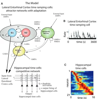
Figure 1. Model of the Lateral Entorhinal Cor-tex Temporal Cells and Hippocampal Time Cells
(A) The lateral entorhinal cortex temporal cells and hippocampal time cells. The lateral entorhinal cortex is modeled as an integrate-and-fire attrac-tor neuronal network. The excitaattrac-tory neurons are divided into two selective populations or pools, S1 and S2, either of which can sustain a high-firing rate attractor state because of strong syn-aptic connectionsw+within each population. The
inhibitory neurons ensure that only one population, S1 or S2, can be active at any one time. In the model, there are three such attractor networks for the lateral entorhinal cortex, each with a different time constant for the synaptic depression that occurs in the recurrent collaterals of the attractors networks (indicated by recurrent arrows), so that nets 1–3 tend to cycle with different periods (long, medium, and short). The S1 and S2 pools of all three lateral entorhinal cortex attractor networks send their outputs to a competitive network in the hippocampus (e.g., in CA1 or in the dentate gyrus). The competitive network learns to respond to combinations of the outputs of the lateral entorhi-nal cortex and forms thereby hippocampal time cells, as shown in the simulations.
(B) Example of a lateral entorhinal cortex time ramping cell recorded in the rat byTsao et al. (2018). The firing rate is in spikes per second. These neu-rons are characterized by slow ramping changes in their firing rates with a long time period. (Repro-duced with permission of Springer Nature.) (C) Hippocampal time cells recorded in the rat by
cortex grid cell firing into hippocampal place cell firing (Rolls et al., 2006), suitable in a parallel way for object-place associa-tions, and reflecting it is suggested the conservatism in brain design (Rolls, 2016). The overall architecture is illustrated in Figure 1.
The Model of Lateral Entorhinal Cortex Temporal Cells and Hippocampal Time Cells
The theory was tested, illustrated, and analyzed in a simulation that provided a model shown inFigure 1with biologically plau-sible characteristics. The lateral entorhinal cortex was modeled as three networks, each with an integrate-and-fire attractor neuronal network with synaptic adaptation in the recurrent collateral synapses (Rolls and Deco 2016). In the model as simu-lated, there are three such attractor networks for the lateral ento-rhinal cortex, each with a different time constant for the synaptic depression that occurs in the recurrent collaterals of the attractor networks, so that nets 1–3 tend to cycle with different periods (long, medium, and short). Our aim is to investigate these mech-anisms in a biophysically realistic attractor framework, so that the properties of receptors, synaptic currents, and the statistical effects related to the probabilistic spiking of the neurons can be part of the model. We use a minimal architecture, a single attrac-tor or autoassociation network (Amit, 1989; Deco et al., 2013; Hopfield, 1982; Rolls, 2016; Rolls and Deco, 2010; Rolls and Treves, 1998). We chose a recurrent (attractor) integrate-and-fire network model that includes synaptic channels for AMPA, NMDA, and GABAA receptors (Brunel and Wang, 2001) and
synaptic adaptation, which has been extensively described (Deco and Rolls, 2005; Deco et al., 2013; Rolls, 2016; Rolls and Deco, 2010) and is described in detail in theSTAR Methods. The S1 and S2 pools of all three lateral entorhinal cortex attrac-tor networks send their outputs to a competitive network in the hippocampus (e.g., in CA1 or in the dentate gyrus;Rolls, 2016, 2018) (Figure 1). The competitive network learns to respond to combinations of the outputs of the lateral entorhinal cortex and forms thereby hippocampal time cells, as shown in the simula-tions. A description of the operation and properties of competi-tive networks, together with demonstration simulation software, is provided inRolls (2016), and the details of the implementation are described in theSTAR Methods. The fully connected two-layer lateral entorhinal cortex (LEC)-hippocampal model has the architecture of a competitive network. There is an input layer of six lateral entorhinal cortex temporal cell populations (S1 and S2 from nets 1–3) with feedforward associatively modifiable synaptic connections onto an output layer of 20 hippocampal cells (Figure 1).
Operation of the Network over a Long Timescale
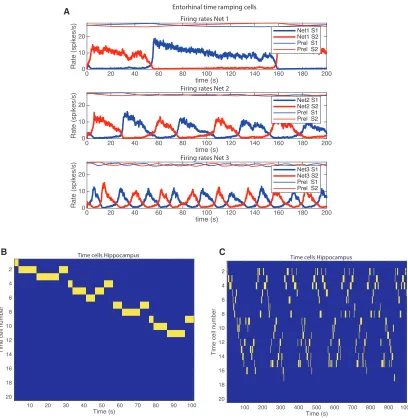
Figure 2A shows a simulation of the lateral entorhinal cortex model with an intermediate value for the time constant of the synaptic adaptation set byfD= 0.99960 for net 2. The firing rates
in nets 1–3 are shown, and within each network, the firing rates of the population of neurons in S1 and S2 are shown. For net 1, fD= 0.99972, producing a longer time constant for the synaptic
depression and longer cycle times for the firing of net 1. For net 3,fD= 0.99800, producing a shorter time constant for the
synaptic depression and shorter cycle times for the firing of net 3.
Figure 2B shows the firing of the hippocampal (e.g., CA1) neu-rons in the same simulation. The hippocampal neuneu-rons have been sorted so that the neuron that fires first in the sequence is in the top row. Each vertical yellow line represents firing by a hippocampal neuron. The first 100 s of the simulation is shown. Figure 2C shows the simulation of the firing of the hippocampal (e.g., CA1) neurons as illustrated inFigure 2B, but now for the full 1,000 s of the simulation. An interesting point emerges, that the hippocampal neurons come back into activity again later on. This is also found by neurons recorded in the lateral entorhinal cortex (Tsao et al., 2018). However,Figure 2C also shows that a reasonable approximation of the 120 s sequence repeats later on in the time period of 1,000 s. This is evidence that the whole system is generating a time signature that is reasonably sta-ble over the whole 1,000 s time period, in that components of the sequence are replayed later on in time. This ‘‘replay’’ is more evident in the simulations for shorter time periods described next.
Operation of the Network at a Shorter Timescale Useful over a 10 s Period
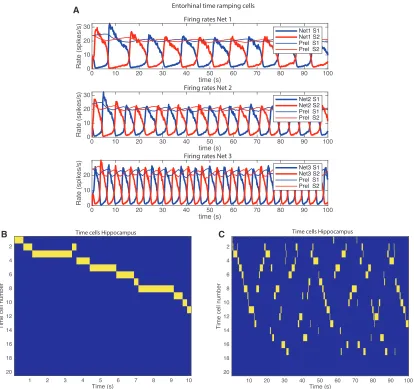
To test whether the network system could provide useful tempo-ral encoding for the order of sevetempo-ral items to be remembered over a 10 s period, the simulations described were repeated but with a shorter timescale for the synaptic depression factor fD, as shown inFigure 3. The simulations show that the system
could provide useful temporal encoding for the order of several items to be remembered over a 10 s period.Figure 3B shows that for the first 10 s of the hippocampal (CA1) cell firing (for the simulation illustrated in Figure 3A), different hippocampal neurons fired sequentially at different times in the first 10 s. That provides a basis for the hippocampus to associate different objects with different times in even a short period of 10 s and later to recall the items in the correct order (Kesner and Rolls, 2015; Rolls, 2018). The representations provided here by the hippocampus are orthogonal.
Figure 3C shows the hippocampal (CA1) cell firing for the whole 100 s period of the simulation illustrated inFigure 3B. This shows that the hippocampal cells are active not just in the first period after the simulation is started (or reset by an environmental event such as the start of a trial). However,Figure 3C also shows that a reasonable approximation of the 10 s sequence repeats twice in the time period of 100 s. This is further evidence that the whole system is generating a time signature that is reasonably stable over the whole 100 s time period, in that components of the sequence are replayed later on in time. There is even evidence of ‘‘reverse replay,’’ evident for example in the period 10–20 s, in which the sequence is repeated in reverse order. Part of the importance of these simulations at a shorter timescale is that some of the tests of the effects of hippocampal lesions on sequence learning have spanned times in the order of 10 s (Kesner and Rolls, 2015), and also many of the task-related sequential firing of hippocampal neurons has been found over short time-scales in the order of 10 s of seconds (Eichenbaum, 2014, 2017; Howard and Eichenbaum, 2015; MacDonald et al., 2011).
what appears to be a similar temporal sequence of neuronal firing may be repeated and may even occur in reverse order. To inves-tigate whether this is a robust emergent property of this neuronal architecture, we ran the same competitive network simulations but replaced the firing of the integrate-and-fire neurons (illustrated inFigures 3C and2A) with precisely generated waveforms, for example, square waves as shown inFigure 4A. An example of perfect play and reverse replay is shown inFigure 4B.
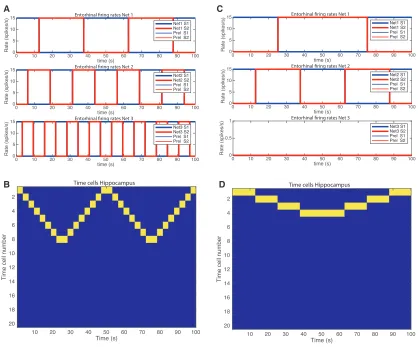
We explain the mechanism usingFigures 4C and 4D with a simplified system in which only nets 1 and 2 of the entorhinal
cor-tex are active (Figure 4C).Figure 4D shows that neuron 1 had learned to respond to the combination of net 1 population S1 firing, and net 2 population S1 firing. Neuron 2 had learned to respond to net 1 S1 and net 2 S2. Neuron 3 had learned to respond to net 1 S2 and net 2 S2. Neuron 4 had learned to respond to net 1 S2 and net 2 S1. It is now possible to see that these combinations of firing in nets 1 and 2 then occur in reverse sequence, generating the reverse replay in the hippocampal neurons. Only four neurons are needed to encode the combina-tions of firing in nets 1 and 2, and no other hippocampal neurons
C B
[image:5.603.100.508.98.516.2]A
Figure 2. Simulation of the Model with a Long Value for the Time Constant Set byfD= 0.99960 for Net 2
(A) The firing rates in nets 1–3 are shown, and within each network, the firing rates of the population of neurons in S1 and S2 are shown. In addition, the value of the variablePrelfor pools S1 and S2 is shown, scaled so that a value ofPrel= 1 is shown as 30 on the y axis. For net 1,fD= 0.99972, producing a longer time constant
for the synaptic depression and longer cycle times for the firing of net 1. For net 3,fD= 0.99800, producing a shorter time constant for the synaptic depression and
shorter cycle times for the firing of net 3. The first 200 s period of a 600 s simulation in which similar firing continued is shown.
have learned to respond, because this is a competitive network (as described byRolls, 2016).
We found that robust replay and reverse replay could be generated if a wide variety of waveforms, including square, sine, triangular, and sawtooth waves, were presented to the competitive network. The replay and reverse replay occur when the waveforms in nets 1–3 are only approximate harmonics of each other, and for a range of different phases, with the result-ing hippocampal neurons then becomresult-ing more noisy in their for-ward and reverse replay, similar to what is illustrated inFigures
3C and 2C. In some cases only forward replay is seen, for
example, if square or sine waveforms in nets 1–3 are locked at zero phase difference (which would only occur in the unlikely case that the waveforms in nets 1–3 were perfect harmonics of each other). We note that both are at the same rate as in the original sequence. We consider in theDiscussionthe relation between this emergent property of this architecture, with the
re-ports of rapid replay and reverse replay of sequences of time cell firing that can occur during sharp waves in the rodent hippocam-pus (Foster, 2017; Foster and Wilson, 2006).
Furthermore, it is not necessary to have two populations S1 and S2 in approximate antiphase in any given net: just a single oscillating waveform, in just for example S1, suffices. (Two pop-ulations in approximate antiphase in a given net in the lateral entorhinal cortex is part of the model by which regular periodicity is produced in the lateral entorhinal cortex but is not needed for the operation of the hippocampal competitive network.)
These analyses show that it is a natural property of the architec-ture described here that it can produce replay and reverse replay.
DISCUSSION
The theory is proposed that lateral entorhinal cortex temporal encoding cells, with their very slow firing rate time courses A
[image:6.603.93.507.99.488.2]B C
Figure 3. Simulation of the Model with Shorter Values for the Time Constants Set byfD= 0.996 for Net 2,fD= 0.998 for Net 1, andfD= 0.992 for Net 3
that may gradually decrease, or increase, over often very many seconds, are implemented by attractor networks with adapta-tion with a time course of many seconds. Competing attractor populations within a single network are set up so that typically one attractor population is active, and as a result of adaptation, its firing becomes less, allowing the other population (or popu-lations in the brain) within a network to climb into activity for some time. Over time, the two populations tend to cycle in alternation. To provide for a diversity and richness of timescales that can be encoded by the lateral entorhinal cortex, the theory is that there are several separate networks within the lateral entorhinal cortex, with each one set to have different parame-ters for the temporal adaptation, so that the different networks cycle with different timescales. The theory is that within the lateral entorhinal cortex there are at least three different net-works with different time constants for the adaptation, with
the longer time constant networks deeper in the entorhinal cortex, consistent with the empirical evidence for the medial entorhinal cortex (Giocomo et al., 2011; Kropff and Treves, 2008). Weak coupling between the nets potentially allows them by weak interactions to influence each other, helping make the whole system more reliable in its timing because each network is less likely to drift because of noise factors independently of the other networks. The theory we propose is that the use of adaptation present in synapses or neurons is one way in which time-related activity can be implemented in a neuronal system, but that the resulting type of encoding has very broad temporal tuning, because of the very slow changes in the firing rates of the lateral entorhinal cortex neu-rons and is not sufficiently sparse and discrete to enable asso-ciation in a hippocampal attractor network in CA3 with other items such as objects, people, etc. (Rolls, 2016, 2018).
A C
[image:7.603.97.515.98.445.2]B D
Figure 4. Simulations to Show How Replay and Reverse Replay Can Be Generated
(A) Simulated square waves for the lateral entorhinal cortex for nets 1–3, with frequencies of 2 for net 1, 4 for net 2, and 8 for net 3.
(B) The hippocampal neurons produced by the lateral entorhinal cortex firing in (A) have been sorted so that the neuron that fires first in the sequence is in the top row. Each vertical yellow line represents firing by a hippocampal neuron. After the initial sequence in which eight neurons come into successive firing, from 0–25 s, there is a period of reverse replay from 25–50 s. This is followed by a repetition of the initial forward sequence from 50–75 s, and this is followed by reverse replay of the sequence from 75–100 s.
(C) Simulated square waves for the lateral entorhinal cortex for nets 1 and 2, with frequencies of 1 for net 1 and 2 for net 2 and no firing for net 3.
The second part of the theory is therefore that the lateral ento-rhinal cortex neuronal firing needs to be converted into a sparse representation in the hippocampus, with different hippocampal neurons responding at discrete times, as has been observed (Eichenbaum, 2014, 2017; Howard and Eichenbaum, 2015; Kraus et al., 2013; Salz et al., 2016). It is proposed here that this conversion is performed by a competitive network (Rolls, 2016) in the hippocampus (in the dentate, CA3, and/or CA1). The theory holds that the competitive network would set up, in hippocampal neurons, representations produced by combina-tions of the firing in the different lateral entorhinal cortex net-works and would make these combination representations relatively discrete and uncorrelated with one another, which is a requirement for efficient operation of autoassociation or attrac-tor networks that associate together different inputs, as shown by analytic investigations (Amit, 1989; Rolls, 2016; Rolls and Treves, 1998; Treves and Rolls, 1991, 1992). This proposal has the advantage that it parallels the theory for how a competitive network can perform a similar computation to convert medial entorhinal cortex spatial grid cell firing (Moser et al., 2014, 2015; Schlesiger et al., 2018) into hippocampal place cell firing (Rolls et al., 2006). The overall architecture is illustrated in Fig-ure 1. Although the CA1 cells have the appropriate architectFig-ure for a competitive network (Rolls, 2016, 2018) and are implicated in temporal sequence encoding (Kesner and Rolls, 2015), the dentate granule cells also have the appropriate architecture for a competitive network (Rolls, 2016, 2018), and if they were involved in this learning of time cells, that would be advanta-geous, for then the time cell representation would be available for CA3 neurons to associate with objects by autoassociation (Rolls, 2016, 2018). Consistent with this proposal, time cells are found in the CA3 hippocampal neurons as well as in CA1 (Salz et al., 2016).
The theory was tested as described here with an integrate-and-fire simulation of attractor networks (Brunel and Wang, 2001) with synaptic adaptation (Rolls and Deco, 2016). The sim-ulations illustrated inFigures 2A and3A show how the system can operate. One interesting point is that the timescales of the lateral entorhinal cortex firing can be long, with for example 100 s illustrated inFigure 2A, provided that the synaptic depres-sion time constant is long. Consistent with this, a range of synap-tic depression time constants is found for different corsynap-tical neuron types (Markram et al., 2015). A prediction of the research described here is that, at least under natural conditions, some synapses between pyramidal cells in the lateral entorhinal cortex should show long time constants for their synaptic depression. (An alternative mechanism would be neuronal adaptation with a long time constant implemented by calcium entering a cell with a spike and affecting cation channels [Deco and Rolls, 2005; Rolls, 2016; see alsoLiu et al., 2019, who used a similar neuronal adaptation model, and investigated inverse Laplace transforms in a three-layer network].) It is also interesting that although the attractor network modeled normally has binary firing rates (high when in the attractor) (Brunel and Wang, 2001; Deco et al., 2013; Rolls and Deco, 2010), the inclusion of synap-tic adaptation leads to a wide range of graded firing rates (see Figures 2A and3A), and this is another way in which graded firing rates can be produced in the attractor networks found in the
cerebral cortex (Franco et al., 2007; Lim et al., 2015; Pereira and Brunel, 2018; Rolls, 2016; Rolls and Treves, 2011; Treves, 1990; Treves and Rolls, 1991).
Another interesting point learned from the simulations is that in order to reduce noise, so that the timing is reliable and the tran-sition times between the attractor states are reliable, the network needs to be quite large. In our simulations, the noise or variability in the neuronal firing was reduced by using each network with 5,000 neurons. At this size of network, the noise still may have some effect (perhaps for example in net 1 inFigure 2). In the brain of course the networks may be larger, but some variability in the slow firing of lateral entorhinal neurons is evident, as in Figure 2B, cell 7, ofTsao et al. (2018), shown inFigure 1B. A feature of the simulations described here is how similar the firing of the simulated lateral entorhinal cortex cells is to that illustrated in Figure 2B, cell 7, ofTsao et al. (2018)for the rat lateral entorhinal cortex.
A useful property illustrated by the simulations is that not only do the hippocampal time cells in the simulations provide a sparse representation with the firing of different hippocampal neurons relatively uncorrelated, but the simulations show that the hippocampal neuronal activity must represent combinations of the firing of the lateral entorhinal cortex neurons. This is shown by the fact that the dimensionality of the lateral entorhinal cortex firing is just three (one for each of the three networks), yet many more than this number of hippocampal neurons are formed by self-organizing competitive learning to represent different times (typically the number of binary combinations, i.e., eight). The the-ory is that the different timescales of different lateral entorhinal cortex neurons allow a wide range of times to be encoded by hippocampal neurons that learn to respond to different combina-tions of the firing of entorhinal time ramping cells.
An interesting point learned from the simulations was that not only did hippocampal time cells have an initial period of sequen-tial firing in the first period after the simulation is started (or reset by an environmental event such as the start of a trial), as illus-trated inFigure 2B, but also had activity later on in time, which appears to reflect ‘‘replay’’ (Figure 2C). A fascinating finding was thatFigure 3C also shows that a reasonable approximation of the 10 s sequence repeats twice in the time period of 100 s. This is evidence that the whole system is generating a time signature that is reasonably stable over the whole time period, in that components of the sequence are replayed later on in time. There is even evidence of ‘‘reverse replay,’’ evident for example in the period 10–20 s of Figure 3C, in which the sequence is repeated in reverse order. The simulations shown
inFigures 4A–4D show how this replay and reverse replay is
The replay and reverse replay described here are at the same rate as in the original sequence, because they are controlled by the time ramping cells of the lateral entorhinal cortex. We propose that the much more rapid replay and reverse replay described so far in the hippocampus, occurring over sometimes 200 ms for the whole sequence, may be playback from the recurrent collateral CA3 attractor network, which once it has been presented with replay and reverse replay temporal se-quences, may play them back at high speed determined primar-ily by the synaptic delay time constants in the recurrent collateral CA3–CA3 attractor network (Rolls, 2016; Sompolinsky and Kanter, 1986).
It is interesting that the CA1 cells of the hippocampus send projections back to the entorhinal cortex (Kesner and Rolls, 2015; Rolls, 2016, 2018). This provides an interesting possibility for feedback from the hippocampal time cell population to influ-ence the lateral entorhinal cortex time ramping cell neurons, and this could be a mechanism for stabilizing the whole system against drift or of extending the duration over which time can be encoded. However, we envisage that the robust operation of the system for timescales of seconds to many minutes is facil-itated by resetting the activity of the neurons at the start of a task in which sequential information must be encoded, and evidence consistent with this hypothesis was found for lateral entorhinal cortex neurons (Tsao et al., 2018).
Overall, the work described here provides a further important step in understanding the operation of the hippocampus, by showing how temporal encoding could be formed in the lateral entorhinal cortex, how this code is not suitable for an associative episodic memory system such as is believed to be implemented in the hippocampus, and how time cells found in the hippocam-pus could be produced, with an appropriately sparse and orthogonal representation of time for use in a hippocampal mem-ory system that can associate place and/or time with objects to encode and later retrieve episodic memories (Kesner and Rolls, 2015; Rolls, 2016, 2018). It has been suggested that learning temporal sequences of events is an important function of the hippocampus (Buzsa´ki and Tingley, 2018; Kesner and Rolls, 2015), and the research described here shows how synaptic adaptation taking place over time in the lateral entorhinal cortex can then lead to neurons that are appropriate for learning tempo-ral sequences in the hippocampus (Rolls, 2016). Moreover, a clear and quantitative mechanism for how hippocampo-cortical back-projections could lead to the recall of information in the neocortex has been described (Rolls, 1989, 2016, 2018; Treves and Rolls, 1994), and that recall to the neocortex can be in the correct temporal sequence as a result of the hippocampal sys-tem mechanisms described here.
In conclusion, the concepts introduced in this research pro-vide a foundational approach to a major issue in neuroscience, the mechanisms by which time is encoded in the brain and how the time representations are then useful in the hippocampal episodic memory of events and their temporal order.
STAR+METHODS
Detailed methods are provided in the online version of this paper and include the following:
d KEY RESOURCES TABLE
d LEAD CONTACT AND MATERIALS AVAILABILITY
d METHOD DETAILS
B Attractor Networks for the Lateral Entorhinal Cortex Ramping Neurons
B Implementation of Neural and Synaptic Dynamics
B Connection Matrices
B Short Term Synaptic Depression
B The Model Parameters Used in the Simulations
B The Competitive Network Used to Model the Trans-form from Entorhinal Time Ramping Cells to Hippo-campal Time Cells
d QUANTIFICATION AND STATISTICAL ANALYSIS
d DATA AND CODE AVAILABILITY
ACKNOWLEDGMENTS
This research was supported by the Oxford Centre for Computational Neuro-science. We gratefully acknowledge the use of the image fragment shown in
Figure 1B fromTsao et al. (2018)and of the image shown inFigure 1C from
Kraus et al. (2013). Permission was obtained for both.
AUTHOR CONTRIBUTIONS
E.T.R. produced the theory and model, designed the research, wrote the code, performed the simulations, and wrote the paper. P.M. added to the code and performed simulations to analyze the parameter space.
DECLARATION OF INTERESTS
The authors declare no competing interests. E.T.R. is also a Specially Ap-pointed Professor at Fudan University, Institute of Science and Technology for Brain-inspired Intelligence, Shanghai, China.
Received: March 6, 2019 Revised: May 30, 2019 Accepted: July 14, 2019 Published: August 13, 2019
REFERENCES
Abeles, M. (1991). Corticonics—Neural Circuits of the Cerebral Cortex (Cam-bridge University Press).
Amit, D.J. (1989). Modeling Brain Function (Cambridge University Press).
Braitenberg, V., and Sch€utz, A. (1991). Anatomy of the Cortex (Springer-Verlag).
Brunel, N., and Wang, X.J. (2001). Effects of neuromodulation in a cortical network model of object working memory dominated by recurrent inhibition. J. Comput. Neurosci.11, 63–85.
Buzsa´ki, G., and Tingley, D. (2018). Space and time: the hippocampus as a sequence generator. Trends Cogn. Sci.22, 853–869.
Dayan, P., and Abbott, L.F. (2001). Theoretical Neuroscience (MIT Press).
Deco, G., and Rolls, E.T. (2005). Sequential memory: a putative neural and syn-aptic dynamical mechanism. J. Cogn. Neurosci.17, 294–307.
Deco, G., Rolls, E.T., Albantakis, L., and Romo, R. (2013). Brain mechanisms for perceptual and reward-related decision-making. Prog. Neurobiol. 103, 194–213.
Eichenbaum, H. (2014). Time cells in the hippocampus: a new dimension for mapping memories. Nat. Rev. Neurosci.15, 732–744.
Eichenbaum, H. (2017). On the integration of space, time, and memory. Neuron95, 1007–1018.
Foster, D.J., and Wilson, M.A. (2006). Reverse replay of behavioural se-quences in hippocampal place cells during the awake state. Nature440, 680–683.
Franco, L., Rolls, E.T., Aggelopoulos, N.C., and Jerez, J.M. (2007). Neuronal selectivity, population sparseness, and ergodicity in the inferior temporal visual cortex. Biol. Cybern.96, 547–560.
Giocomo, L.M., Moser, M.B., and Moser, E.I. (2011). Computational models of grid cells. Neuron71, 589–603.
Hartley, T., Lever, C., Burgess, N., and O’Keefe, J. (2013). Space in the brain: how the hippocampal formation supports spatial cognition. Philos. Trans. R. Soc. Lond. B Biol. Sci.369, 20120510.
Hertz, J., Krogh, A., and Palmer, R.G. (1991). An Introduction to the Theory of Neural Computation (Addison-Wesley).
Hestrin, S., Sah, P., and Nicoll, R.A. (1990). Mechanisms generating the time course of dual component excitatory synaptic currents recorded in hippocam-pal slices. Neuron5, 247–253.
Heys, J.G., and Dombeck, D.A. (2018). Evidence for a subcircuit in medial entorhinal cortex representing elapsed time during immobility. Nat. Neurosci.
21, 1574–1582.
Hopfield, J.J. (1982). Neural networks and physical systems with emergent collective computational abilities. Proc. Natl. Acad. Sci. U S A79, 2554–2558.
Howard, M.W., and Eichenbaum, H. (2015). Time and space in the hippocam-pus. Brain Res.1621, 345–354.
Howard, M.W., Viskontas, I.V., Shankar, K.H., and Fried, I. (2012). Ensembles of human MTL neurons ‘‘jump back in time’’ in response to a repeated stim-ulus. Hippocampus22, 1833–1847.
Jahr, C.E., and Stevens, C.F. (1990). Voltage dependence of NMDA-activated macroscopic conductances predicted by single-channel kinetics. J. Neurosci.
10, 3178–3182.
Kesner, R.P., and Rolls, E.T. (2015). A computational theory of hippocampal function, and tests of the theory: new developments. Neurosci. Biobehav. Rev.48, 92–147.
Koch, K.W., and Fuster, J.M. (1989). Unit activity in monkey parietal cortex related to haptic perception and temporary memory. Exp. Brain Res.76, 292–306.
Kraus, B.J., Robinson, R.J., 2nd, White, J.A., Eichenbaum, H., and Hasselmo, M.E. (2013). Hippocampal ‘‘time cells’’: time versus path integration. Neuron
78, 1090–1101.
Kropff, E., and Treves, A. (2008). The emergence of grid cells: intelligent design or just adaptation? Hippocampus18, 1256–1269.
Lehn, H., Steffenach, H.A., van Strien, N.M., Veltman, D.J., Witter, M.P., and Ha˚berg, A.K. (2009). A specific role of the human hippocampus in recall of tem-poral sequences. J. Neurosci.29, 3475–3484.
Levy, W.B. (1985). Associative changes in the synapse: LTP in the hippocam-pus. In Synaptic Modification, Neuron Selectivity, and Nervous System Organization, W.B. Levy, J.A. Anderson, and S. Lehmkuhle, eds. (Erlbaum), pp. 5–33.
Levy, W.B., and Desmond, N.L. (1985). The rules of elemental synaptic plasticity. In Synaptic Modification, Neuron Selectivity, and Nervous System Organization, W.B. Levy, J.A. Anderson, and S. Lehmkuhle, eds. (Erlbaum), pp. 105–121.
Lim, S., McKee, J.L., Woloszyn, L., Amit, Y., Freedman, D.J., Sheinberg, D.L., and Brunel, N. (2015). Inferring learning rules from distributions of firing rates in cortical neurons. Nat. Neurosci.18, 1804–1810.
Liu, Y., Tiganj, Z., Hasselmo, M.E., and Howard, M.W. (2019). A neural micro-circuit model for a scalable scale-invariant representation of time. Hippocam-pus29, 260–274.
MacDonald, C.J., Lepage, K.Q., Eden, U.T., and Eichenbaum, H. (2011). Hippocampal ‘‘time cells’’ bridge the gap in memory for discontiguous events. Neuron71, 737–749.
Markram, H., Muller, E., Ramaswamy, S., Reimann, M.W., Abdellah, M., Sanchez, C.A., Ailamaki, A., Alonso-Nanclares, L., Antille, N., Arsever, S.,
et al. (2015). Reconstruction and Simulation of Neocortical Microcircuitry. Cell163, 456–492.
Markus, E.J., Barnes, C.A., McNaughton, B.L., Gladden, V.L., and Skaggs, W.E. (1994). Spatial information content and reliability of hippocampal CA1 neurons: effects of visual input. Hippocampus4, 410–421.
McCormick, D.A., Connors, B.W., Lighthall, J.W., and Prince, D.A. (1985). Comparative electrophysiology of pyramidal and sparsely spiny stellate neu-rons of the neocortex. J. Neurophysiol.54, 782–806.
Moser, E.I., Roudi, Y., Witter, M.P., Kentros, C., Bonhoeffer, T., and Moser, M.B. (2014). Grid cells and cortical representation. Nat. Rev. Neurosci.15, 466–481.
Moser, M.B., Rowland, D.C., and Moser, E.I. (2015). Place cells, grid cells, and memory. Cold Spring Harb. Perspect. Biol.7, a021808.
O’Keefe, J. (1979). A review of the hippocampal place cells. Prog. Neurobiol.
13, 419–439.
O’Neill, M.E. (2014). PCG: A family of simple fast space-efficient statis-tically good algorithms for random number generation. Technical Report, HMC-CS-2014-0905 (Harvey Mudd College). https://www.cs.hmc.edu/tr/ hmc-cs-2014-0905.pdf.
Oja, E. (1982). A simplified neuron model as a principal component analyzer. J. Math. Biol.15, 267–273.
Pereira, U., and Brunel, N. (2018). Attractor dynamics in networks with learning rules inferred from in vivo data. Neuron99, 227–238.e4.
Rolls, E.T. (1989). Functions of neuronal networks in the hippocampus and neocortex in memory. In Neural Models of Plasticity: Experimental and Theoretical Approaches, J.H. Byrne and W.O. Berry, eds. (Academic Press), pp. 240–265.
Rolls, E.T. (2016). Cerebral Cortex: Principles of Operation (Oxford University Press).
Rolls, E.T. (2018). The storage and recall of memories in the hippocampo-cortical system. Cell Tissue Res.373, 577–604.
Rolls, E.T., and Deco, G. (2010). The Noisy Brain: Stochastic Dynamics as a Principle of Brain Function (Oxford University Press).
Rolls, E.T., and Deco, G. (2016). Non-reward neural mechanisms in the orbito-frontal cortex. Cortex83, 27–38.
Rolls, E.T., and Treves, A. (1998). Neural Networks and Brain Function (Oxford University Press).
Rolls, E.T., and Treves, A. (2011). The neuronal encoding of information in the brain. Prog. Neurobiol.95, 448–490.
Rolls, E.T., and Wirth, S. (2018). Spatial representations in the primate hippo-campus, and their functions in memory and navigation. Prog. Neurobiol.171, 90–113.
Rolls, E.T., Stringer, S.M., and Elliot, T. (2006). Entorhinal cortex grid cells can map to hippocampal place cells by competitive learning. Network17, 447–465.
Rolls, E.T., Grabenhorst, F., and Deco, G. (2010). Choice, difficulty, and con-fidence in the brain. Neuroimage53, 694–706.
Salin, P.A., and Prince, D.A. (1996). Spontaneous GABAA receptor-mediated inhibitory currents in adult rat somatosensory cortex. J. Neurophysiol.75, 1573–1588.
Salz, D.M., Tiganj, Z., Khasnabish, S., Kohley, A., Sheehan, D., Howard, M.W., and Eichenbaum, H. (2016). Time cells in hippocampal area CA3. J. Neurosci.
36, 7476–7484.
Schlesiger, M.I., Boublil, B.L., Hales, J.B., Leutgeb, J.K., and Leutgeb, S. (2018). Hippocampal global remapping can occur without input from the medial entorhinal cortex. Cell Rep.22, 3152–3159.
Sompolinsky, H., and Kanter, I. (1986). Temporal association in asymmetric neural networks. Phys. Rev. Lett.57, 2861–2864.
Spruston, N., Jonas, P., and Sakmann, B. (1995). Dendritic glutamate receptor channels in rat hippocampal CA3 and CA1 pyramidal neurons. J. Physiol.482, 325–352.
Treves, A., and Rolls, E.T. (1991). What determines the capacity of autoasso-ciative memories in the brain? Network2, 371–397.
Treves, A., and Rolls, E.T. (1992). Computational constraints suggest the need for two distinct input systems to the hippocampal CA3 network. Hippocampus
2, 189–199.
Treves, A., and Rolls, E.T. (1994). Computational analysis of the role of the hip-pocampus in memory. Hiphip-pocampus4, 374–391.
Tsao, A., Sugar, J., Lu, L., Wang, C., Knierim, J.J., Moser, M.B., and Moser, E.I. (2018). Integrating time from experience in the lateral entorhinal cortex. Nature
561, 57–62.
Tuckwell, H. (1988). Introduction to Theoretical Neurobiology (Cambridge Uni-versity Press).
Wang, X.J. (2002). Probabilistic decision making by slow reverberation in cortical circuits. Neuron36, 955–968.
Wilson, F.A., O’Scalaidhe, S.P., and Goldman-Rakic, P.S. (1994). Functional syn-ergism between putative gamma-aminobutyrate-containing neurons and pyra-midal neurons in prefrontal cortex. Proc. Natl. Acad. Sci. U S A91, 4009–4013.
STAR
+
METHODS
KEY RESOURCES TABLE
LEAD CONTACT AND MATERIALS AVAILABILITY
Requests for further information should be directed to and will be fulfilled by the Lead Contact, Edmund Rolls (Edmund.Rolls@oxcns. org). This study did not generate new unique reagents.
METHOD DETAILS
The model of lateral entorhinal cortex temporal cells and hippocampal time cells
The theory was tested, illustrated, and analyzed in a simulation that provided a model shown inFigure 1with biologically plausible characteristics. The lateral entorhinal cortex was modeled as three networks, each with an integrate-and-fire attractor neuronal network with synaptic adaptation in the recurrent collateral synapses (Rolls and Deco 2016). Each of the three networks contains 5000 neurons, of which 4000 are in the excitatory pools and 1000 are in the inhibitory pool IH. The excitatory neurons of each network were divided into two selective populations or pools S1 and S2 either of which can sustain a high firing rate attractor state (Figure 1a). Each population S1 and S2 each with 1800 neurons have strong intra-pool connection strengthsw+. There is a small non-selective pool (NS) (with 400 neurons) which does not respond in the model, but is included in this class of model to reflect the fact that there is a contribution from other neurons in a brain area to the noisy inputs to a neuron from other neurons to which it is connected (Brunel and Wang, 2001; Rolls and Deco, 2010). The other connection strengths are 1 or weakw. Every neuron in the network also receives inputs from 800 external neurons, and these neurons have firing rates that are continuously applied to both pools S1 and S2. The inhibitory neurons ensure that only one population, S1, or S2, can be active with a high firing rate at any one time.
In the model as simulated, there are three such attractor networks for the lateral entorhinal cortex, each with different time con-stants for the synaptic depression that occurs in the recurrent collaterals of the attractor networks, so that nets 1–3 tend to cycle with different periods (long, medium, and short). Our aim is to investigate these mechanisms in a biophysically realistic attractor framework, so that the properties of receptors, synaptic currents and the statistical effects related to the probabilistic spiking of the neurons can be part of the model. We use a minimal architecture, a single attractor or autoassociation network (Amit, 1989; Deco et al., 2013; Hertz et al., 1991; Hopfield, 1982; Rolls, 2016; Rolls and Deco, 2010; Rolls and Treves, 1998). We chose a recurrent (attractor) integrate-and-fire network model which includes synaptic channels for AMPA, NMDA and GABAAreceptors (Brunel and
Wang, 2001) which has been extensively described (Deco et al., 2013; Rolls, 2016; Rolls and Deco, 2010), and is described in detail below. The three attractor networks that model the entorhinal cortex each had different synaptic depression time constants, so that the three networks cycled with different timescales, in order to provide a rich diversity of time information. (In the brain, there could of course be more than three networks each with its own timescale). The three attractor networks were weakly coupled with symmet-rical connections between populations S1 of all three networks, and populations S2 of all 3 networks, with coupling parameter wcouplingbetween the three networks set to 0.001, which was a value greater than 0 that just enabled Nets 1, 2 and 3 to interact,
as tested by cross-correlations between the firing rates of the neurons in the three networks. The concept was that this weak coupling would allow rich interactions between the three attractor networks that were likely to be beneficial in helping them to interact weakly in time to make the whole system more robust against temporal drift in any of the networks, or the starting conditions.
To implement the synaptic adaptation, a synaptic depression mechanism was used for the recurrent collateral connections between the neurons in each specific pool, i.e., within S1 or within S2, followingDayan and Abbott (2001), page 185 andDeco and Rolls (2005). In particular, the probability of transmitter releasePrelwas decreased after each presynaptic spike by a factor
Prel=Prel,fDwithfD =0:999. Between presynaptic action potentials the release probabilityPrelwas updated by
tP
dPrel
dt =P0Prel
withP0=1 andtP= 25 s unless otherwise stated.
The S1 and S2 pools of all three lateral entorhinal cortex attractor networks send their outputs to a competitive network in the hippocampus (e.g., in CA1 or in the dentate gyrus [Rolls, 2016, 2018]) (Figure 1). The competitive network learns to respond to combinations of the outputs of the lateral entorhinal cortex, and forms thereby hippocampal time cells, as shown in the simulations. A description of the operation and properties of competitive networks, together with demonstration simulation software, is provided
REAGENT or RESOURCE SOURCE IDENTIFIER Software and Algorithms
MATLAB Mathworks Inc R2018a
byRolls (2016), and the details are provided below. The fully connected 2-layer lateral entorhinal cortex (LEC) / hippocampal model has the architecture of a competitive network. There is an input layer of 6 LEC temporal cell populations (S1 and S2 from Nets 1–3) with feedforward associatively modifiable synaptic connections onto an output layer of 20 hippocampal cells.
Attractor Networks for the Lateral Entorhinal Cortex Ramping Neurons Attractor Framework
The aim is to investigate the mechanisms for the ramping neurons in the lateral entorhinal cortex in a biophysically realistic attractor framework, so that the properties of receptors, synaptic currents and the statistical effects related to the probabilistic spiking of the neurons can be part of the model. We use a minimal architecture, a single attractor or autoassociation network (Amit, 1989; Deco et al., 2013; Hertz et al., 1991; Hopfield, 1982; Rolls, 2016; Rolls and Deco, 2010; Rolls and Treves, 1998). We chose a recurrent (attractor) integrate-and-fire network model which includes synaptic channels for AMPA, NMDA and GABAAreceptors (Brunel
and Wang, 2001).
Both excitatory and inhibitory neurons are represented by a leaky integrate-and-fire model (Tuckwell, 1988). The basic state var-iable of a single model neuron is the membrane potential. It decays in time, when the neurons receive no synaptic input, down to a resting potential. When synaptic input causes the membrane potential to reach a threshold, a spike is emitted and the neuron is set to the reset potential at which it is kept for the refractory period. The emitted action potential is propagated to the other neurons in the network. The excitatory neurons transmit their action potentials via the glutamatergic receptors AMPA and NMDA which are both modeled by their effect in producing exponentially decaying currents in the postsynaptic neuron. The rise time of the AMPA current is neglected, because it is typically very short. The NMDA channel is modeled with an alpha function including both a rise and a decay term. In addition, the synaptic function of the NMDA current includes a voltage dependence controlled by the extracellular magne-sium concentration (Jahr and Stevens, 1990). The inhibitory postsynaptic potential is mediated by a GABAAreceptor model and is
described by a decay term.
Each single attractor network contains 4000 excitatory and 1000 inhibitory neurons, which is consistent with the observed propor-tions of pyramidal cells and interneurons in the cerebral cortex (Abeles, 1991; Braitenberg and Sch€utz, 1991; Rolls, 2016). The connection strengths are adjusted using mean-field analysis (Brunel and Wang, 2001; Deco et al., 2013; Rolls, 2016; Rolls and Deco, 2010), so that the excitatory and inhibitory neurons exhibit a spontaneous activity of 3 Hz and 9 Hz, respectively (Koch and Fuster, 1989; Wilson et al., 1994). The recurrent excitation mediated by the AMPA and NMDA receptors is dominated by the NMDA current to avoid instabilities (Wang, 2002).
The attractor network model features a minimal architecture to investigate attractor-related firing and consists of two selective pools, S1 and S2 (Figure 1). We use just two selective pools to eliminate possible disturbing factors. The non-selective pool NS models the spiking of cortical neurons and serves to generate an approximately Poisson spiking dynamics in the model (Brunel and Wang, 2001), which is what is observed in the cortex. The inhibitory pool IH contains the 1000 inhibitory neurons. The connection weights between the neurons within each selective pool or population are called the intra-pool connection strengthsw+ . The increased strength of the intra-pool connections is counterbalanced by the other excitatory connectionsðwÞto keep the average excitatory input constant.
The network receives Poisson input spikes via AMPA receptors which are envisioned to originate from 800 external neurons at an average spontaneous firing rate of 3 Hz from each external neuron, consistent with the spontaneous activity observed in the cerebral cortex (Rolls, 2016; Rolls and Treves, 1998; Wilson et al., 1994). Given that there are 800 synapses on each neuron in the network for these external inputs, the number of spikes being received by every neurons in the network is 2,400 spikes/s. This external input can be altered for specific neuronal populations to introduce the effects of external stimuli on the network. In addi-tion to these external excitatory inputs, each excitatory neuron receives 1800 excitatory inputs from other neurons in the same specific population in which the firing rate is modulated byw+, and 2200 excitatory inputs from other excitatory neurons (given that there are 4000 excitatory neurons) in which the firing rate is modulated byw(seeFigure 1). A detailed mathematical description is provided next.
Implementation of Neural and Synaptic Dynamics
We use the mathematical formulation of the integrate-and-fire neurons and synaptic currents described byBrunel and Wang (2001). Here we provide a brief summary of this framework (Rolls, 2016; Rolls and Deco, 2010, 2016).
The dynamics of the sub-threshold membrane potentialVof a neuron are given by the equation:
Cm
dVðtÞ
dt = gmðVðtÞ VLÞ IsynðtÞ:
Both excitatory and inhibitory neurons have a resting potentialVL=70 mV, a firing thresholdVthr=50 mV and a reset potential
Vreset=55 mV. The membrane parameters are different for both types of neurons: Excitatory (Inhibitory) neurons are modeled with a
membrane capacitanceCm= 0.5 nF (0.2 nF), a leak conductancegm= 25 nS (20 nS), a membrane time constanttm= 20 ms (10 ms),
and a refractory periodtref= 2 ms (1 ms). Values are extracted fromMcCormick et al. (1985).
When the threshold membrane potentialVthris reached, the neuron is set to the reset potentialVreset at which it is kept for a
The network is fully connected withNE= 4000 excitatory neurons andNI= 1000 inhibitory neurons, which is consistent with the
observed proportions of the pyramidal neurons and interneurons in the cerebral cortex (Rolls, 2016). The synaptic current impinging on each neuron is given by the sum of recurrent excitatory currents (IAMPA;recand INMDA;rec), and the external excitatory
currentðIAMPA;extÞ, and the inhibitory currentðIGABAÞ:
IsynðtÞ=IAMPA;extðtÞ+IAMPA;recðtÞ+INMDA;recðtÞ+IGABAðtÞ:
The recurrent excitation is mediated by the AMPA and NMDA receptors, inhibition by GABA receptors. In addition, the neurons are exposed to external Poisson input spike trains mediated by AMPA receptors at a rate of 2.4 kHz. These can be viewed as originating fromNext= 800 external neurons at an average rate of 3 Hz per neuron, consistent with the spontaneous activity observed in the
cerebral cortex (Rolls, 2016). The currents are defined by:
IAMPA;extðtÞ=gAMPA;extðVðtÞ VEÞ
XNext
j=1
SAMPAj ;extðtÞ
IAMPA;recðtÞ=gAMPA;recðVðtÞ VEÞ
XNE
j=1
wAMPA ji s
AMPA;rec j ðtÞ
INMDA;recðtÞ=
gNMDAðVðtÞ VEÞ
1+½Mg+ +expð0:062VðtÞÞ=3:573
XNE
j=1
wNMDA ji sNMDAj ðtÞ
IGABAðtÞ=gGABAðVðtÞ VIÞ
XNI
j=1
wGABA ji s
GABA j ðtÞ
whereVE= 0 mV,VI=70 mV,wjare the synaptic weights,sj’s the fractions of open channels for the different receptors andg’s
the synaptic conductances for the different channels. The NMDA synaptic current depends on the membrane potential and the extracellular concentration of Magnesium (½Mg+ += 1 mM [Jahr and Stevens, 1990]). The values for the synaptic conductances for excitatory neurons aregAMPA;ext= 2.08 nS,gAMPA;rec= 0.104 nS,gNMDA= 0.327 nS andgGABA= 1.25 nS ; and for inhibitory neurons
gAMPA;ext= 1.62 nS,gAMPA;rec= 0.081 nS,gNMDA= 0.258 nS andgGABA= 0.973 nS. These values are obtained from the ones used by
Brunel and Wang (2001)by correcting for the different numbers of neurons. The conductances were calculated so that in an
unstructured network the excitatory neurons have a spontaneous spiking rate of 3 Hz and the inhibitory neurons a spontaneous rate of 9 Hz. The fractions of open channels are described by:
dsAMPAj ;extðtÞ
dt =
sAMPAj ;extðtÞ
tAMPA +
X
k dttk
j
dsAMPAj ;recðtÞ
dt =
sAMPAj ;recðtÞ
tAMPA +
X
k dttk
j
dsNMDA j ðtÞ
dt =
sNMDA j ðtÞ
tNMDA;decay+a
xjðtÞ
1sNMDA j ðtÞ
dxjðtÞ
dt =
xjðtÞ
tNMDA;rise+
X
k dttk
j
dsGABA j ðtÞ
dt =
sGABA j ðtÞ
tGABA +
X
k d
ttkj
wheretNMDA;decay= 100 ms is the decay time for NMDA synapses,tAMPA= 2 ms for AMPA synapses (Hestrin et al., 1990; Spruston
et al., 1995) andtGABA= 10 ms for GABA synapses (Salin and Prince, 1996; Xiang et al., 1998);tNMDA;rise= 2 ms is the rise time for
NMDA synapses (the rise times for AMPA and GABA are neglected because they are typically very short) anda= 0.5 ms-1. The sums
overkrepresent a sum over spikes formulated asd-peaksdðtÞemitted by presynaptic neuronjat timetk j.
Connection Matrices
In the following Tables, S1 is one of the specific excitatory populations of neurons, S2 is the other specific excitatory population of neurons, NS is the non-specific excitatory population, and IH is the inhibitory population.
Fraction of pool sizesfi
Connection matrix for AMPA and NMDA – [from, to]
wherew =0:8fS1w+ 0:8fS1
Connection matrix for GABA – [from, to]
Short Term Synaptic Depression
A synaptic depression mechanism was used for the recurrent collateral connections between the neurons in each specific pool, i.e., within S1 or within S2, followingDayan and Abbott (2001), page 185. In particular, the probability of transmitter releasePrelwas
decreased after each presynaptic spike by a factorPrel=Prel,fDwithfD=0:999. Between presynaptic action potentials the release
probabilityPrelwas updated by
tP
dPrel
dt =P0Prel
withP0=1 andtP= 25 s unless otherwise stated.
The Model Parameters Used in the Simulations
The fixed parameters of the model are shown in the Table below, and not only provide information about the values of the parameters used in the simulations, but also enable them to be compared to experimentally measured values. The variable parameters in the simulations were as follows, with the values used as described next unless otherwise stated.
The recurrent collateral connection strengthw+was set to a value just sufficiently high to maintain the activity of a population of neurons firing reliably if the firing rate was high, yet to make the attractor less stable if the firing rate decreased because of synaptic adaptation in the recurrent collateral synapses, resulting in the other attractor population of neurons within a single network in their unadapted state rise up into a high firing rate attractor state. That value ofw+was 1.34. This helps maintain the activity of one of the attractor populations S1 and S2 sufficiently excitable that one population would tend to be active. The external input to the neurons in the network was 0.0035 (i.e., 3.35 Hz per each of 800 synapses for these external Poisson inputs, or a total barrage of an average of 2,800 spikes/s received by each neuron). (These external inputs were the same for populations S1 and S2, and correspond to the lvalues used in a decision-making attractor network [Rolls, 2016; Rolls and Deco, 2010; Rolls et al., 2010].)
fDwhich sets the rate of decay of the synaptic depression for the recurrent collateral connections in pools S1 and S2 was set to
0.999 for net 2. (In other words, the synaptic strength was reduced by 0.001 of its existing value for every spike received at a synapse.) This value was multiplied by 5 for net 3 to make it cycle faster; and was multiplied by 0.7 for net 1 to make it cycle slower. It was found
S1 S2 NS IH
0.36 0.36 0.08 0.2
Values are relative to all neurons, not only the excitatory portion.
S1 S2 NS IH
S1 w+ w 1 1
S2 w w+ 1 1
NS w w 1 1
IH 0 0 0 0
S1 S2 NS IH
S1 0 0 0 0
S2 0 0 0 0
NS 0 0 0 0
IH 1 1 1 1
that the system could be set to different timescales by alteringfDin the range 0.99 to 0.9996. The valuetPadjusts how rapidly across
time (independently of spiking activity)Prelreturns back up toward its maximal value of 1.0.tPwas set to a low value of 1 / (2e-5) unless
otherwise stated, corresponding to 50 s, that resulted inPrelclimbing in the absence of neuronal firing back to its baseline over many
seconds. (If Net 3 was required to cycle fast because of its value forfD, then it was helpful to settPto 1 / (4e-5) to help the synaptic
depression to recover more rapidly in time for the next cycle.)
The inhibition synaptic connection parameter for the IH neurons was set to a value to keep the peak firing rate relatively low, to be compatible with the low firing rates of lateral entorhinal cortex neurons with rates that change slowly over time (Tsao et al., 2018), and to achieve strong competition between the populations S1 and S2 (seeFigure 1) in a network, so that only one population was active at any one time. The value used was 1.23 unless otherwise stated.
The coupling parameterwcouplingbetween the three networks was set to 0.001, which was a value greater than 0 that just enabled
Nets 1, 2 and 3 to interact, as tested by cross-correlations between the firing rates of the neurons in the three networks. Table: Parameters used in the integrate-and-fire simulations
The Competitive Network Used to Model the Transform from Entorhinal Time Ramping Cells to Hippocampal Time Cells
The neural network architecture is shown inFigure 1, and a full description of the operation and properties of competitive networks, together with simulation software, is provided byRolls (2016). The fully connected 2-layer lateral entorhinal cortex (LEC) / hippocam-pal model has the architecture of a competitive network. There is an input layer of 6 LEC temporal cell populations (S1 and S2 from Nets 1–3) with feedforward associatively modifiable synaptic connections onto an output layer of 20 hippocampal cells.
NE 800
NI 200
r 0.1
w+ 1.34
wI 1.23
Next 800
next 2.4 kHz
Cm(excitatory) 0.5 nF
Cm(inhibitory) 0.2 nF
gm(excitatory) 25 nS
gm(inhibitory) 20 nS
VL 70 mV
Vthr 50 mV
Vreset 55 mV
VE 0 mV
VI 70 mV
gAMPA;ext(excitatory) 2.08 nS
gAMPA;rec(excitatory) 0.104 nS / N
gNMDA(excitatory) 0.327 nS / N
gGABA(excitatory) 1.25 nS / N
gAMPA;ext(inhibitory) 1.62 nS
gAMPA;rec(inhibitory) 0.081 nS / N
gNMDA(inhibitory) 0.258 nS / N
gGABA(inhibitory) 0.973 nS / N
tNMDA;decay 100 ms
tNMDA;rise 2 ms
tAMPA 2 ms
tGABA 10 ms
The competitive network model receives inputs from 6 populations of LEC temporal cells with three different characteristic time courses of their firing. There are 20 output neurons in the competitive network. The activity at 400 time steps of the LEC simulation was used to train the hippocampal competitive network. Activity from the LEC layer is propagated through the feedforward synaptic connections to activate a set of cells in the hippocampal layer. (The synaptic weights from the EC to hippocampal cells are initially set to random values. This is standard in competitive networks, and ensures that some firing of output cells will be produced by the inputs, with each output cell likely to fire at a different rate for any one input stimulus.) The activations of the cells in the hippocampal layer are calculated according to
hhippi =
X
j
wijxLECj
wherehhippi is the activation of hippocampal celli,xLEC
j is the firing rate of LEC cell populationj, andwijis the synaptic weight from LEC
celljto hippocampal celli. Next, mutual inhibition between the hippocampal cells implements competition to ensure that there is only a small winning set of hippocampal cells left active. The mutual inhibition (which would be implemented by inhibitory feedback neu-rons which implement lateral inhibition in the brain) ensures that the sparseness of the activity in the hippocampal layer is kept to a fixed value, set in the simulations to 0.01. (In the simulations the competition was achieved by first setting the firing rates to the square of the activations – corresponding to the steeply rising part of a sigmoid activation function – and second by feedback adjustment of the threshold of the firing until the desired sparseness was achieved. The sparsenessaof the representation can be measured, by extending the binary notion of the proportion of neurons that are firing, as
a=
PN
i=1
yi=N
2
PN i=1
y2
i
N
whereyiis the firing rate of theith neuron in the set ofNneurons.) The algorithm was thus set to adjust the threshold for the firing of
neurons until a sparseness of 0.01 was reached. With the graded firing rates of the neurons, the result was that typically the proportion of neurons with non-zero firing rates after the competition was numerically somewhat larger than the sparseness value given as a parameter to the network.
Next, the synaptic weights between the active LEC cells and the active hippocampal cells are strengthened according to the associative Hebb learning rule
dwij=kyihippxLECj
wheredwijis the change of synaptic weight andkis the learning rate constant.kwas set to be sufficiently low that weight vectors
learned early in training were not overwritten by the end of training. To prevent the same few neurons always winning the competition, the synaptic weight vectors are set to unit length after the learning at each location. (To implement weight normalization the synaptic
weights were rescaled to ensure that for each hippocampal celliwe have ffiffiffiffiffiffiffiffiffiffiffiffiffiffiffiffiffiP
j ð
wijÞ2
r
=1, where the sum is over all LEC cellsj.) Such a
renormalization process may be achieved in biological systems through heterosynaptic long- term depression that depends on the existing value of the synaptic weight (Oja, 1982; Rolls, 2016; Rolls and Treves, 1998). (Heterosynaptic long-term depression was described in the brain byLevy [1985]andLevy and Desmond [1985].)
QUANTIFICATION AND STATISTICAL ANALYSIS
All simulations were run with different random seeds, to ensure that the Figures illustrate the properties of the networks.
DATA AND CODE AVAILABILITY
No new data were generated. Code to show the operation of the systems described here is described byRolls (2016)and is available