Holistic virtual machine scheduling in cloud datacenters towards minimizing total energy

Holistic Virtual Machine Scheduling in Cloud

Datacenters towards Minimizing Total Energy

Xiang Li, Peter Garraghan, Xiaohong Jiang, Zhaohui Wu and Jie Xu, Member, IEEE

Abstract—Energy consumed by Cloud datacenters has dramatically increased, driven by rapid uptake of applications and services globally provisioned through virtualization. By applying energy-aware virtual machine scheduling, Cloud providers are able to achieve enhanced energy efficiency and reduced operation cost. Energy consumption of datacenters consists of computing energy and cooling energy. However, due to the complexity of energy and thermal modeling of realistic Cloud datacenter operation, traditional approaches are unable to provide a comprehensive in-depth solution for virtual machine scheduling which encompasses both computing and cooling energy. This paper addresses this challenge by presenting an elaborate thermal model that analyzes the temperature distribution of airflow and server CPU. We propose GRANITE – a holistic virtual machine scheduling algorithm capable of minimizing total datacenter energy consumption. The algorithm is evaluated against other existing workload scheduling algorithms MaxUtil, TASA, IQR and Random using real Cloud workload characteristics extracted from Google datacenter tracelog. Results demonstrate that GRANITE consumes 4.3% - 43.6% less total energy in comparison to the state-of-the-art, and reduces the probability of critical temperature violation by 99.2% with 0.17% SLA violation rate as the performance penalty.

Index Terms—Cloud computing; energy efficiency; datacenter modeling; workload scheduling; virtual machine

——————————  ——————————

1 I

NTRODUCTION

he global uptake of Cloud computing has subsequently driven a dramatic increase in datacenter power con-sumption. Datacenters composed of thousands of inter-connected servers built to provide various Cloud services globally, subsequently consuming enormous amount of energy. In the past ten years, Google servers’ electricity de-mand has increased approximately 20 fold [1], accouting for nearly 1% of all electricity use for the world [2]. A study within 2011 [2] shows that the energy used by datacenters increased by 36% in US and 56% worldwide from 2005 - 2010, accounting for 2% and 1.3% of total electricity use, respectively. The energy consumption is expected to in-crease continuesly during the coming years, and it is sup-ported by [3], predicting that a global annual datacenter construction size for 2020 will be $78 billion. In addition to high operational costs, a range of problems manifest due to high energy consumption and heat density including re-duced system reliability, degraded service performance and environmental deterioration [3].

Datacenter energy usage can be categorized as stem-ming from computing and cooling, with the latter forstem-ming 43% of the total energy consumption as reported in [4]. On one hand, server computing energy consumption of un-derutilized resources accounts for a substantial amount of the actual energy use, particularly in Cloud environments [5]. For this reason, server consolidation is often used to

achieve enhanced computing energy efficiency[6], [7], and functions by scheduling workloads to fewer servers and shutting down idle servers (or put them into sleep mode). On the other hand, due to the skewed temperature distri-bution (i.e. cooling must address the hottest server), work-load balancing becomes an important consideration [8], [9] to reduce cooling energy draw. This is achieved by distrib-uting workload evenly amongst servers to minimize the highest temperature in order to avoid hot spots. The anal-ysis results in opposing objectives from the perspective of workload scheduling: load consolidation attempts to de-crease the number of active servers to save computing en-ergy, however consolidation onto fewer servers can form hot spots which results in higher cooling energy require-ment. Load balancing attempts to avoid hot spots however more active servers operating at lower utilization can con-sume unnecessary computing power.

Furthermore, with the rapid development of virtualiza-tion technology and the emergence of Cloud computing paradigm, a large number of future-generation datacenters use virtualization technology allowing dynamic resource scaling and migration. As a result, it is imperative to ad-dress the scheduling of Virtual Machines (VMs) consider-ing both computconsider-ing and coolconsider-ing energy. However, this is challenging as it requires in-depth interdisciplinary knowledge of computing, fluid mechanics and thermody-namics. Firstly, fine-grained models capturing the Com-puter Room Air Conditioner (CRAC), airflow and server have to be developed and evaluated to lay the foundation for algorithm design. Secondly, these models should be in-tegrated into an energy-aware scheduling algorithm ex-ploiting datacenter characteristics that minimizes the total energy consumption while adhering to performance over-heads within an acceptable range dictated by the Service

xxxx-xxxx/0x/$xx.00 © 200x IEEE Published by the IEEE Computer Society

T

————————————————

 Xiang Li, Xianghong Jiang and Zhaohui Wu are with the Department of Computer Science and Technology, Zhejiang University, Hangzhou 310027, China.

E-mail: {lixiang2011, jiangxh, wzh}@zju.edu.cn

 Peter Garraghan: is with School of Computing & Communications, Lancaster University, LA1 4WA, UK.

E-mail: [email protected]

 Jie Xu is with the School of Computing, University of Leeds, Leeds LS2 9JT, UK.

Level Agreement (SLA). Finally, in order to evaluate such an algorithm, it is also necessary to conduct experiments in order for evaluation against other algorithms in terms of energy efficiency, system availability and reliability. Our paper addresses these challenges and the main contribu-tions can be summarized as follows.

̶ Cooling models capturing thermal features of CRACs, air and servers within datacenters holistically. We describe the

methodology of defining the model parameters with Computational Fluid Dynamics (CFD) technique. We further implement the models in Cloud simulator to demonstrate its usage. To the best of our knowledge, this is the first paper addresses server CPU temperature considering cooling infrastructure, datacenter layout and server workload in a dynamic and holistic manner.

̶ Virtual machine placement and migration algorithm to min-imize total energy. We present GRANITE - a VM

sched-uling algorithm for reducing holistic datacenter energy consumption. We consider both initial VM placement and dynamic live migration to achieve better energy ef-ficiency. Our algorithm explicitly takes account of en-ergy consumed by cooling devices and servers.

̶ Algorithm performance evaluation in comparison with other algorithms. Four representative energy-aware

schedul-ing algorithms are selected for comparschedul-ing GRANITE. Experiments demonstrate that it can achieve 43.6% less than the worst algorithm and 4.3% less than the second best algorithm in terms of total energy, and maintain the SLA violation in an acceptable range.

The remainder of this paper is organized as follows. Sec-tion 2 gives the background and the challenges of this work. Section 3 describes the problem statement and the holistic datacenter modeling. Section 4 presents the methodology of model parameter identification. Section 5 details our greedy based VM scheduling algorithm. Section 6 presents the performance results. Section 7 surveys the precious work on energy-aware management and Section 8 dis-cusses the conclusions and further research directions.

2 B

ACKGROUND

2.1 Datacenter Energy Characteristics

The location of hot recirculation regions within in the facil-ity and the mixing pattern of hot rack exhaust air with the cold supply air are key issues in datacenter thermal man-agement. There are several candidate configurations avail-able for the air ducting designs for datacenters [10], re-ferred as Supply and Return Schema. Without loss of gen-erality, we consider the “raised floor & ceiling return” schema, which is demonstrated as the best option in data-center design. In this scenario, cold air supplied by CRACs passes through the raised floor plenum to cool computing equipment within the datacenter. Assuming the datacenter comprises  CRACs, represented by



AC AC

1

,

2

,

,

AC



,





C

A (1)

in which ACi is the i-th CRAC. Cold air supplied by CRACs enter each rack through the inlet and flows out from the rear, removing the heat generated by computing servers as hot air. The space between two inlet sides is known as the cold aisle, while the space between two outlet sides is

called hot aisle [11], [12]. Hot air eventually is exhausted through return vents locating near the ceiling. A typical Cloud datacenter provides services using virtualization technology such as Xen, KVM or VMware. The workload from users during time interval [t1, t2] is a sequence

com-prising  VMs, and the workload is scheduled among 

servers  within the datacenter. We represent the work-load  and servers  by:





1 2

1, 2, , ,

t t

VM VM VM



 

V _V (2)



PM PM

1

,

2

,

,

PM



.





P

M (3)

Generally, any specific VM scheduling solution  dur-ing time interval [t1, t2] can be represented as Equation (4),

including initial placement  and dynamic migration  [13].





















 

 

 









 

1 2

1 2

1 2

1 2

, ,

, ,..., ,

, ,..., ,

where

, ,

, .

t t

i i

t t i

PM VM PM VM PM VM

PM PM PM

PM VM PM

i





  

  

 



V

W

S I G

I

G O O O

O

W V O

P P

V

(4)

The scheduling system will initiate a newly arriving vir-tual machine VMi within a server according to a specific algorithm. The initial placement stage  is represented as a map from the VMs to servers, and PM(VMi) is the place-ment for VMi. In migration stage , the status of all servers are checked at a regular interval. The scheduling system selects a virtual machine subset  comprising  VMs which are migrated from their original host server to an-other server, denoted by PM(i). For algorithms which do not consider VM migration [14], [15],  is configured as null. Total energy required to operate a datacenter is con-sidered as the sum of computing energy Ecomputing and cool-ing energy Ecooling [16], [17], which are considered as energy

TABLE1

SYMBOLS AND DEFINITIONS

Symbol Definition

, , ,  Sets of CRACs, VMs, servers and tasks , , ,  Numbers of CRACs, VMs, servers and tasks AC Abbreviation of CRAC

t Time [s]

, ,  Scheduling solution _{ment stage and (2) } includes: (1) , initial place-, dynamic migration stage PM, VM Abbreviation of servers and virtual machines E Energy consumption [kWh]

Є Configuration / capacity of CPU, memory, etc. u, θ Task CPU utilization and length [instructions] λ Task submission rate

P Power consumption [W] T Temperature [K]

QAC Heat removed by CRACs [J]

w Rotation speed of the fan [r/s]

Rk Temperature raise of rack k by air recirculation [K]

C (Specific) heat capacity [J/K, J/(kg*K)] R Thermal resistance [K/W]

comp/fan CRAC compressor unit / fan unit sup CRAC supply air

consumption by servers and CRACs in this paper, respec-tively. That is,

1 2 1 2 1 2

.

t t t t t t total computing cooling

E E E

  



 (5)

Each specific VM scheduling solution  corresponds to a workload distribution and server utilization profiles that determine the server energy consumption. Therefore the computing energy Ecomputing is a function of . On the other hand, the cooling efficiency is positively correlated with its Supply Air Temperature (SAT, Tsup) [8], [18]. However, Tsup should be set low enough to keep the server temperatures under their critical temperatures [16], [19]. Generally, higher server temperature requires lower Tsup to cool down. Meanwhile, server temperature is affected by its workload status which is a function of scheduling . Therefore, scheduling solution  determines cooling energy in an in-direct manner. Given the workload and datacenter thermal characteristics, we represent the energy consumption as

 

 

.

total computing cooling

E



E

S



E

S

(6)

2.2 Challenges in Total-Energy-Aware Scheduling

Equation (6) indicates a necessity to consider both compu-ting and cooling operation together in order to reduce total datacenter energy. However, this is challenging due to complicated relationship between Ecomputing and Ecoooling [20]. There traditionally exist two different perspectives for en-ergy-aware scheduling in datacenters: computing [5], [15] and cooling [8], [21]. On one hand, minimizing computing energy typically involves consolidating workloads into fewer servers, however results in increased likelihood of high temperature hot spots [16] needing additional cooling energy for removal. On the other hand, the problems of minimizing cooling energy and the highest server temper-ature are shown to be equivalent [18]. Therefore, minimiz-ing coolminimiz-ing energy entails workload balancminimiz-ing. However this results in more active servers yielding higher compu-ting energy. More formally, assuming that ’ and ’’ are

scheduling solutions that produce the minimum compu-ting energy and cooling energy, respectively.

 

 

 

 

min ,

min .

computing computing cooling cooling

E ' E

E '' E

 

 _{ }

 

 _{ }

S S

S S

(7)

However, solutions that produce localized optimization value do not necessarily achieve the globally minimized value. In order to achieve the best energy efficiency in terms of total energy, we attempt to find the global optimi-zation solution S that

 

 

min





,

however

and

computing cooling total

E

E

E

'

''.









S

S

S

S

S

S

(8)

In other words, uncoordinated scheduling algorithms that consider minimizing computing and cooling energy usage as isolated optimization problems do not necessarily result in the minimal total datacenter energy [17], [20]. Therefore it is critical for energy-aware workload schedul-ing to consider computschedul-ing and coolschedul-ing energy as a sschedul-ingle optimization problem to ascertain an optimal trade-off point and achieve the best energy efficiency.

Another challenge is developing fine-grained simula-tion environment with holistic models. Computing energy modeling has been studied in detail [5], [16]. Traditional CFD technique has been intensively studied [22], [23], but is not applicable for online scheduling due to its time-con-suming characteristic. CloudSim [24], [25] is one of the most powerful simulation platforms for Cloud computing. However, an existing limitation of CloudSim is the inabil-ity to provide models of cooling infrastructures within dat-acenters. Prior to algorithm design, it is necessary to imple-ment the cooling models presented in this paper. In order to make simulation results more convincing, we compare the model outputs with CFD modeling results. Further-more, we try to use real measured parameters to define our models, such as the workload from real Google datacenter tracelog, real server power profiles, etc.

3 C

LOUD

D

ATACENTER

M

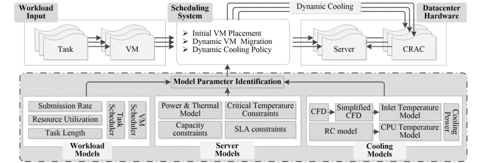
ODELING

In this section, we introduce the models our solution is based on, followed by the problem statement targeted by our paper. Fig. 1 illustrates the overall architecture of our methodology. Users submit tasks deployed within VMs. The scheduling system is responsible for VM placement and migration. Furthermore, it dynamically adjusts CRAC capacity in order to reduce cooling costs. Decision making of the scheduling system is based on the models identified off-line, including workload models, server models and cooling models. The variables and parameters used in the modeling are presented within Table 1.

3.1 Workload Models

Assume that during any time interval [t1, t2], the workload

comprises  VMs, presented in Equation (2). More specifi-cally, the configuration of each VM is represented by



, ,



, [1, 2,..., ],

VM i core mips memory

Є  Є Є Є i V (9)

in which ЄVM i is the configuration of i-th VM. Each VM in-cluds the number of VCPU (Єcore), core processing speed

(Єmips) and memory size (Єmemory). In each VM, we deploy

the tasks submitted by users. In other words, we consider the scenario that tasks are deployed in VMs rather than di-rectly in servers. Each server hosts one or more VMs at any given time. The corresponding VM is instantiated when deploying a task and destroyed after finishing the task. The task sequence submitted by users is represented by





 

2 1 2

1, , , ,

, , [1, 2,..., ],

t t

i

task task task task u i



 

 

T _K

K

(10)

where  is the number of all tasks, and each task is repre-sented by CPU utilization u and length θ (instructions). As-suming that each VM runs a single task, we have  = . The tasks are submitted according to a submission rate λ, which is a function of time denoted by

 

.

submission

f

t





(11)

The total number of submitted tasks are the integral of submission rate if we consider the submission rate as a continuous function, we have

 

2

1 .

t

submission t f t dt



_

3.2 Server Models

Assuming the datacenter comprises  heterogeneous servers shown in Equation (3) with different CPU capacity, memory size, etc. Given the workload during time interval [t1, t2] and the server status at time t1, a specific scheduling

solution  will produce corresponding workload distribu-tion and server status. The CPU utilizadistribu-tion is as follows.

 

t





u

PM1

 

t u

,

PM2

 

t

,



,

u

PM

 

t



,

t



 

t t

1

,

2

,

U

_M (13)

where uPM1(t) is the CPU utilization of i-th PM at time t. Server power consumption is primarily dependant on CPU utilization. In practical terms, we use the power mod-els of HP ProLiant ML110 G4 and G5 [25], which define the power consumption at {0%, 10%, …, 100%}. Power at the utilization at any interval is modelled by a segmented lin-ear function. Server status is defined as active and inactive. A server utilization greater than 0% indicates that a server is active. An inactive server (sleep mode, turned off) results in power utilization equals to 0, requiring ignorable energy. The computing power of all servers at time t is given by

 



 





 



1 1

.

i i

PM i PM i

PM PM i i

i i

P t P u t P t

 

 





M 



M U (14)

The energy of all servers within a datacenter during time interval [t1, t2] is obtained by

 

2

1

. t

PM t PM

E 



P t dt (15)

Meanwhile, resources required by all VMs that run on server i cannot exceed its capacity ЄPM i, since we donnot use oversubscription technique [15], [25]. Therefore a fea-sible scheduling algorithm mush satisfy

in

,

[1, 2,...,

].

VMs PM i PM i

Є



Є

i





M

(16)

Additionally, in order to ensure that the servers will not overheat and eventually fail, it is necessary to maintain server temperature under the critical threshold (Tcritical) at all times [19], satisfying

 

t



,

PM critical

T

T

(17)

where TPM and Tcritical are bold, representing vectors of server temperatures and their critical temperatures. Nu-merous works [16], [17], [19] consider inlet air temperature

Tinlet as TPM while [12], [26] consider the CPU temperature

Tcpu as TPM. We argue that inlet temperature is an insuffi-cient performance indicator as thermal management target is indicated by CPU temperature. As a result, this paper focuses on CPU temperature as analysis objective.

An important aspect for Cloud providers is the set of Quality of Service (QoS) guarantees. This is commonly re-ferred as a SLA [27]. In this paper, we consider the con-straints of SLA as follows [25].



R



ˆ,

v A R

SLA  CPU CPU CPU S (18)

in which SLAv is a metric to evaluate the level of violation in SLA, and Sˆ is the maximum acceptable threshold. CPUR and CPUA are the CPU capacity required by users and actual allocation by the Cloud system, respectively.

3.3 Cooling Models

We consider the CRACs as the only cooling devices since it accounts for the most cooling energy [4]. The energy con-sumed by each CRAC during time interval [t1, t2]

com-prises compressor (i.e. a component of the CARC, respon-sible for air compression) energy and fan energy [10], [11].

1 2 1 2 1 2

.

t t t t t t AC comp fan

E E E

  



 (19)

The power consumption of a fan unit is proportional to the cubic of its rotation speed w, and the energy consump-tion is obtained by time integral of the power. The energy consumed by the compressor is given by

 

1 2 1 2

,

t t t t

comp AC sup E Q CoP T

 

 (20)

where Qt1ACt2



is the heat removed by the CRAC, which can be modelled according to server energy [19] or the heat dis-parity between datacenter out flow and CRAC supply air [11]. CoP is the Coefficient of Performance [8], [11]. A higher CoP indicates a more efficient process, requiring less work to remove a constant amount of heat. Research shows a positive correlation between CoP and supply air temperature (Tsup) [8]:

2

0.0068

sup

0.008

sup

0.458.

CoP





T





T



(21)

[image:4.567.39.514.63.226.2]

constraints shown in Equation (17). In order to understand the relationship between CPU temperature and Tsup, we propose a two-step temperature model. The first step is

rack inlet temperature modeling considering both CRAC

status and datacenter layout. The second step is CPU

tem-perature modeling that factors server thermal

characteris-tics and its respective workload. The airflow of the inlet air is a mix of recirculated hot air exhausted from other serv-ers and supplied cool air from CRACs. The time-discrete form of rack inlet temperature is as follows [9], [28]:





 

 



 

 



 

, , , , 1 ,

inlet k inlet k

j k j sup, j inlet k k j

T t t T t

g w t T t T t r t



  





A     (22)

where Tinlet, k(t+Δt) and Tinlet, k(t) are the inlet temperature of rack k at time step t+1 and t, respectively. gj, k quantifies the influences of the cooling settings of CRAC j to rack k, in-cluding supply air temperature Tsup, j and the fan speed wj. In our paper, we consider fan speed as a constant. We focus on the optimization of the supply air temperature to con-duct thermal management. Here rk(t) is a time-varying item, representing the temperature effect of recirculated hot air. However, previous work lacks detailed analysis to identify rk(t). Here we introduce our approach to model the rack inlet temperature and identify rk(t) based on Equation (22) as follows.

Within a scenario of stable airflow pattern in a datacen-ter, according to [16], [19] the inlet temperature of rack k

( ,

stable inlet k

T ) is the weighted sum of supply air temperature (Tsup) of each CRAC and the recirculation influence. Theoreti-cally, ,

stable inlet k

T is influenced by all the working CRAC units within the datacenter. However as observed from [9], rack inlet temperature is predominately affected by a selected small number of CRAC units. In this paper, we only con-sider the closest CRAC (numbered as 0). The supply air temperature and the fan speed are denoted as Tsup,0 and w0, respectively. The temperature raise of rack k imposed by recirculated influence derives from exhausted air of all the other racks, denoted by Rk. We have

,

.

stable

inlet k sup,0 k

T



T



R

(23)

Assume that g0,k in Equation (22) is a time-ste p-propor-tional parameter shown as follows, defining the tempera-ture impact from CRAC status.

 

0,k 0 0

,

g



w t



g' w

 

t



G'





t

(24) where g’and G’ are constants. A differential equation to capture the dynamics of inlet temperature based on Equa-tion (22) and its soluEqua-tion is shown below,





 

 





, , , , .

inlet k inlet k stable inlet k inlet k

T t dt T t

G' dt T T t

  

    (25)

 



 



, , ,

0

,

,

Solution:

stable stable

inlet k inlet k inlet k inlet t k

c

T

t



T



T



T

e

 ₍₂₆₎

where c is a constant, capturing the temperature influence by the closest CRAC unit, and ,

stable inlet k

T is obtained with Equa-tion (23). Tinlet, k(0) is the inlet temperature of rack k at the very beginning. It is now possible to present the complete inlet temperature models. The unknown parameters to be

identified are Rk and c, which will be described in Section 4.2. Next, we can conduct CPU temperature modeling, which is the most important indicator of thermal manage-ment. The RC model shown below is the most established means to obtain CPU temperature [26], [29].

 

_{ }

, cpu cpu inlet t t dT

RC T PR T

dt

    (27)

where R and C are thermal resistance and heat capacity of the server, respectively. Tinlet is obtained with Equation (26). By solving this differential equation, CPU temperature is modelled as follows.

 



0



,

t RC cpu inlet inlet

T t PR T  T PRT e (28)

where and Tcpu(0) is the initial CPU temperature. Equation (28) implies that the stable CPU temperature is PR + Tinlet. The constraint of RC model is that it assumes the CPU power and inlet temperature is constant. However, CPU power depends on its utilization which is time-varying, and rack inlet temperature is dynamic as well described in Equation (26). Our solution is to compute CPU tempera-ture at a regular interval with Equation (26) and (28).

3.4 Problem Statement

We formulate the problem as optimize workload schedul-ing to minimize the total energy consumption, which is presented in Equation (29). Given the status of servers, CRACs and workloads (represented by VMs and deployed tasks), our main target is to find the optimal scheduling so-lution and supply air temperature to minimize the total en-ergy under the constraints of server capacity, SLA and CPU critical temperature.





 

1 2 1 2 1 1

1 2

1 2 1 2 1 2

in : : : , , , , , , ,

, [1, 2,..., ],

, ˆ

t t t t t t

t t

sup t t t t t t

total computing cooling VMs PM i PM i v

S S

T t

E E E

Є Є i

LA           



Given

find and

minimizi

subject d to ng

e :

P C V T

S I G

M

 

T_PM t T_critical.

(29)

4 M

ODEL

P

ARAMETER

I

DENTIFICATION

4.1 Task Parameters

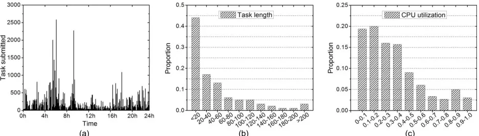
In order to produce realistic models, it is critical to derive parameters from real-world tracelogs. We use the work-load generated by our previous work in [30]. We presented a comprehensive analysis of the workload characteristics derived from Google datacenter that features approxi-mately 25 million tasks. We model the submission charac-teristic of tasks through profiling submission rate hourly. Within each hour, we assume the submission rate follows a random distribution. All users are classified into six clus-ters as shown in [30]. We use the proportion of each cluster as the weight, and the overall submission rate follows the distribution of the weighted sum of these clusters. Then we model tasks with CPU utilization and length via fitted functions provided by our previous work [30]. Fig. 2(a) shows the modelled submission rate with 64,000 tasks. Fig. 2(b) and Fig. 2(c) show the distribution of task length and CPU utilization, respectively. According to our application scenarios, we further make the following assumptions.

Tasks are deployed in VMs rather than directly in servers.

The deployment model of Cloud datacenters with IaaS (In-frastructure as a Service) typically provides Cloud services in terms of virtual machines. In this paper, users are re-quired to initialize VMs and then deploy their tasks within. Resource utilization of each task keeps fluctuating even with fine-grained time interval. For instance, [25] assumes that task utilization varies every fixed interval (e.g. 5 minutes). Since the majority of tasks only utilize tiny pro-portion of resources [30], analysing utilization pattern in the level of task is reasonable. Therefore, in this paper, task utilization is assumed to be stable during its execution.

Availability constraint or communication constraint between VMs are not considered. In order to meet the requirement of

users, VM scheduling is subjected to constraints such as availability constraint and communication constraint. The former is expressed as a combination of anti-colloca-tion/collocation of VMs, implying that corresponding VMs must be placed on the same/different level (e.g. rack). Communication constraint is defined by the bandwidth and latency requirement between two VMs. In our paper, we only focus on VM scheduling under the constraints of server resource showed in Equation (16), which is termed demand constraints [13].

4.2 Rack Inlet Temperature

The advantage of time-discrete model in Equation (22) is

that it simplifies the CFD modeling and captures the rela-tionship between the CRAC cooling capacity and rack inlet temperature [9]. However, [9] does not present sufficient details on parameter identification. In order to identify the parameters Rk and c in Equation (23) and (26) for each rack, we model a datacenter using CFD technique.

The size of our modelled datacenter is 15.8×6.5m2_,

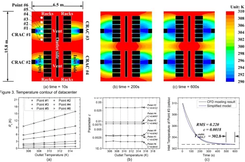
comprising 4 CRACs, 2 vents and 24 rack. The model is 2-dimensional built in Gridgen, including 7,556 cells with the supply air temperature being 290K. The outlet temperature and the initial inlet temperature are configured at 310K. Fig. 3 presents the temperature contour within the datacenter at time 10s, 200s and 600s. We observe that racks near to CRAC units result in lower inlet temperature compared to racks far from CRAC units, showing that datacenter layout imposes great impact on the cooling efficiency of each rack. We also find that there is a significant difference between Fig. 3(a) and Fig. 3(b) in terms of temperature distribution. While the difference between Fig. 3(b) and Fig. 3(c) is not obvious even with wider time gap in comparison with that of Fig. 3(a) and Fig. 3(b), representing that the datacenter becomes stable after certain period of time. From our massive observations, temperature will be stabilized in 500s in majority cases. As a result we identify ,

stable inlet k

T in

Equation (23) as the average temperature after 500s. First, we identify the value of Rk in various of scenarios. Rk is related to the power consumption of servers since re-circulation influence is produced by hot air from each rack. Without loss of generality, we assume that the outlet tem-peratures are identical amongst each rack and ranges in E = [305K, 315K], representing different workload intensities. For each of the workload intensities within range E, we monitor air temperature before entering each rack (inlet temperature) and compute corresponding ,

stable inlet k

T , to deter-mine Rk in Equation (23). Rk is then applied to Equation (26). Parameter c is repeatedly selected within a specific range with step of 0.0001 to produce a profile with Equation (26). Root Mean Square (RMS) errors are computed between the produced profile and the monitored temperature in CFD. This results in selecting c with the minimum RMS.

Using this method, we analyze Rk and c of Point 1-6 (il-lustrated in Fig. 3) under various of outlet temperatures within range E. These points are sufficient to capture the inlet temperatures of all racks since the datacenter is sym-metrical. Fig. 4(a) presents the profile of Rk of each point under different outlet temperatures. We fit each profile

[image:6.567.47.516.62.195.2]

(a) (b) (c)

with a linear function via regression. The R-square is greater than 99.6% and the standard error is within 0.02 in the regression, showing high linearity, which is consistent with the description in [31]. Since we represent different workload intensities in the datacenter via outlet tempera-ture, in practical terms it is necessary to map the workload intensities proportionally into E to determine the corre-sponding Rk. Fig. 4(b) shows the identified parameter c for each level of workload intensities. As illustrated, it is stable under different scenarios. This is due to parameter c is de-pendant on datacenter layout and thermal characteristics. From Fig. 4(a) and Fig. 4(b), we can observe that the points near a CRAC exhibit lower recirculation influence and higher parameter c, indicating higher cooling effi-ciency. Fig. 4(c) shows a case study to demonstrate the practicality of our model. In this case, we set the outlet tem-perature and the initial inlet temtem-perature to 310K, and monitor Point 6 to analyze the model accuracy. First we identify Rk with the regression model shown in Fig. 4(a) and get 12.8K. With Equation (23), stable temperature is determined as 290K+12.7K=302.8K. Parameter c is 0.0018 identified from Fig. 4(b). In comparison with the CFD modeling results, the RMS is 0.220. Our experiments show that the RMS erro rs are under 0.24 in the majority of cases, demonstrating high modeling accuracy.

5 VM

S

CHEDULING

A

LGORITHM

The holistic modeling methodology has been detailed in Section 3, followed by the description of the approach to identify model parameters. Based on the presented models,

we propose our solution to the problem described in Sec-tion 3.4 by introducing GRANITE, a GReedy based

schedul-ing Algorithm miNImizschedul-ing Total Energy. Accordschedul-ingly,

GRANITE contains two stages: (1) initial VM placement 

and (2) dynamic live migration . Meanwhile, the CRAC capacity is dynamically updated to achieve better cooling efficiency: the cooling capacity is adjusted to the lowest ca-pacity (least cooling energy) while maintaining the CPU temperature lower than critical temperature. Our algo-rithm is based on the assumption that for Cloud providers the information of the requests submitted by users, such as the CPU capacity, memory size of each VM and the task utilization is given, or can be predicted. This assumption is widely adopted within the research area [5], [12], [19].

5.1 Initial Placement

In the initial placement stage, GRANITE selects the server with a greedy algorithm. We select the server resulting in the least increase in terms of total power consumption after VM placement. The increase is obtained as follows. First, the total power consumption before placement is given by

1 1

+ .

i i

total PM i AC i

i i

P P P

 

 





M



A (30)

For any submitted VM i, it is necessary to select a

server for its placement. Assume that i is allocated to PM1,

and the CPU utilization of PM1 after allocation is (uPM 1)’. Accordingly, the power cost of PM1 calculated with a

seg-mented linear power model. The CPU temperature is then predicted after allocation during the next time interval (e.g.

[image:7.567.38.531.61.388.2]

(a) time = 10s (b) time = 200s (c) time = 600s

Figure 3. Temperature contour of datacenter

(a) (b) (c)

5 minutes), denoted by (TPM 1)’, with temperature models given in Section 3.3. If (TPM 1)’ is less than its critical tem-perature, CRACs will not be adjusted. Otherwise, the cool-ing capacity of the nearest CRAC is gradually increased by decreasing the SAT, until the predicted (TPM 1)’ is less than the critical temperature. Applying Equation (30) again with updated servers and CRACs, we obtain total power after placing i to PM1, denoted by (Ptotal)’. Similarly, if we place i to PMj, j∈[2, 3, …, ], corresponding total power after placement is obtained. The power increase S is



P

total



'

P

total

,





S

(31)

in which Ptotal and (Ptotal)’ are the total power cost before and after the VM placement, respectively. Our algorithm selects the server with the minimum S as the placement

target. Note that our algorithm will not select servers that result in fully utilized resource after placement, since re-source contention potentially imposes great impact on QoS.

To better illustrate the greedy-based selection of initial placement, we present a case study shown in Fig. 5. VM0 is

submitted to Cloud datacenter, and will be scheduled among 5 servers numbered as 1-5. Allocating VM0 to PM1

will results in overutilized CPU and potential of SLA vio-lation since PM1 is close to full prior to allocation, the

power increase S is regarded as infinite. For PM2 and PM3,

the newly coming VM0 will result in CPU temperature

ex-ceeding the critical threshold. When increasing the cooling capacity, CPU temperature of PM3 can be maintained

un-der critical threshold, while PM2 will be definitely greater

than threshold even with the highest capacity. Therefore,

𝔖 for PM2 is infinite, and 𝔖 for PM3 is the sum of the power

increase of server (ΔPM) and the power increase of the CRAC (ΔCRAC). For PM4 and PM5, 𝔖 is the power increase

of the allocated server (ΔPM) only, since the allocation does not incur critical temperature violation. However, power increase of PM5 (ΔPM) is significantly greater than PM4 due to inactive status before allocation, which

con-sumes negligible energy. Eventually, PM4 will be the

allo-cation target with a power increase of 25W.

5.2 Dynamic Migration

In this stage, live migrations are conducted to balance the

[image:8.567.43.262.60.247.2]

workloads and reduce cooling capacity with its pseudo-code shown in Fig. 6. Dynamic migration is performed at a regular interval. Within each interval, GRANITE checks the status of all servers and defines a temperature old δ. If the server temperature is greater than this thresh-old, one or more VMs will be migrated out. The threshold can be configured to be static or dynamic [25]. The static threshold lacks flexibility in a real Cloud datacenter, which is featured in dynamics and scalability. For this reason, a dynamic threshold is adopted which changes according to specific circumstances. We define the temperature ranking at a certain proportion as the threshold. For instance, we can define the proportion as 10%. Any server with CPU temperature ranks within top 10% is regarded as a hotspot and workload balancing is applied. The VM V with the Figure 5. Initial VM placement in GRANITE

Function dynamicMigration () For: every migration interval

run ()

End Function Function run ()

Rank all servers according to predicted temperature with Equation (28) in descending order. threshold proportion  10%

δ minimum temperature of top 10 percentile of servers

For: each server PM in datacenter

If:PM.Tcpu > δ

workloadBalance ()

End Function

Function workloadBalance ()

While: (PM.Tcpu > δ)

V VM with the minimum utilization within PM PMtarget select a server with the minimum S

migrate V to PMtarget

[image:8.567.285.532.65.251.2]

End Function

Figure 6. Pseudo-code of dynamic migration

(a)

(b)

[image:8.567.304.493.457.730.2]

minimum CPU utilization within the server PM will be se-lected to conduct live migration. The migration target

PMtarget is selected with greedy algorithm similar to the in-itial placement stage. Note that we do not use the widely adopted workload consolidation [6], [7] in GRANITE as the greedy-based algorithm always selects the server with the best energy-efficiency. In other words, energy-efficient servers will be allocated with more workloads which re-sults in the similar effect of consolidation.

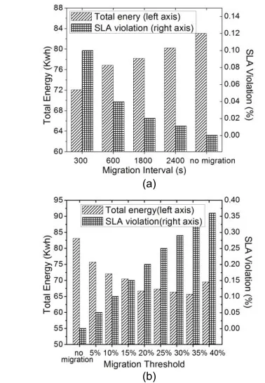
In order to evaluate the performance of dynamic migra-tion. We conducted simulation experiments to demon-strate the impact of migration interval and threshold using the parameters in Table 2. Fig. 7(a) shows that as the mi-gration frequency decreases, we observe an increasing trend in total energy consumption and decreasing trend in SLA violation rate (SLAv, defined in Equation (18)). Since oversubscription is not allowed in our scenario, SLA viola-tion incurs when operating VM live migraviola-tion, which re-sults 10% performance degradation [32]. From the figure we learn that a migration interval should be selected as a trade-off of energy efficiency and performance overhead. Fig. 7(b) shows the impact of different thresholds propor-tion within 0%-40%. Higher threshold proporpropor-tion requires more VM migration leading to higher SLA violation rate. This results in more balance temperature distribution, re-quiring more computing energy and less cooling energy.

6 E

XPERIMENT

R

ESULTS

6.1 Baseline Algorithms

To better illustrate the effectiveness of our algorithm GRANITE, we evaluated it against three representative scheduling algorithms: (1) MaxUtil [5] that attempts to minimize only computing energy by allocating workloads to the server with the maximum average utilization, (2) TASA [12] that tries to minimize only cooling energy by allocating workloads to the current coolest server, (3) IQR [25] considersing both computing and cooling energy, and

(4) Random algorithm. We implemented the above algo-rithms within CloudSim V.3.0.3.

(1) MaxUtil (Maximize Utilization), it aims to consolidate workloads through intensifying the utilization of a small number of resources to reduce computing energy draw. Specifically, it defines a cost function as follows.

 

0

, ₁ 0

,

i j _t i

f





_

u

t



(32)

where 𝜏0 is the processing time of task j. The function value fi,j of task j on server i captures the average utilization dur-ing the task execution. For a given task, MaxUtil checks every servers from the first rack to the last, and selects the server with highest function value as scheduling target.

(2) TASA (Thermal Aware Scheduling Algorithm), it sched-ules workload uniformly to minimize the maximum tem-perature, which is a common approach to reduce the cool-ing capacity requirement and achieve coolcool-ing efficiency. The main idea of TASA is to schedule the “hottest” task prior to “coolest” task to the “coolest” server. In our exper-iment, the real-time schedule system has to allocate the submitted task immediately to meet the QoS. Therefore, we simplify TASA by allocating each task to the server with lowest CPU temperature without considering the task-temperature profile such as “cool task” and “hot task”.

(3) IQR (InterQuartile Range based scheduling), it also con-sists of initial placement phase and dynamic migration phase. For initial placement, it allocates each VM to the server that produces the least computing power increment. In the dynamic migration phase, it conducts live migration at a regular interval to balance workloads. To identify the servers to be balanced, it checks if the server utilization is greater than the upper threshold Tu:

1 ,

u

T   s IQR (33)

where IQR is the midspread or middle fifty, repre-senteding a measure of statistical dispersion, being equal to the difference between the third and first quartiles, shown as follows. The parameter s∈+ defines how ag-gressively the system balance workloads. A greater value for s results in more servers becoming balanced.

(4) Random, randomly places VMs to the servers which can accommodate them (i.e. available capacity). Apart from initial placement, we further conduct VM migration to improve its energy efficiency described in Section 5.2.

6.2 Experiment Result

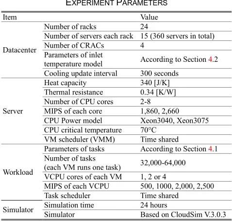
The parameters for constructing the experiment are shown in Table 2. Simulation parameters are configured identi-cally for each algorithm to make the comparison, including datacenter hardware, workloads and simulation environ-ment. Additionally, we set proportional threshold as 20%, and migration interval as 300 seconds in GRANITE.

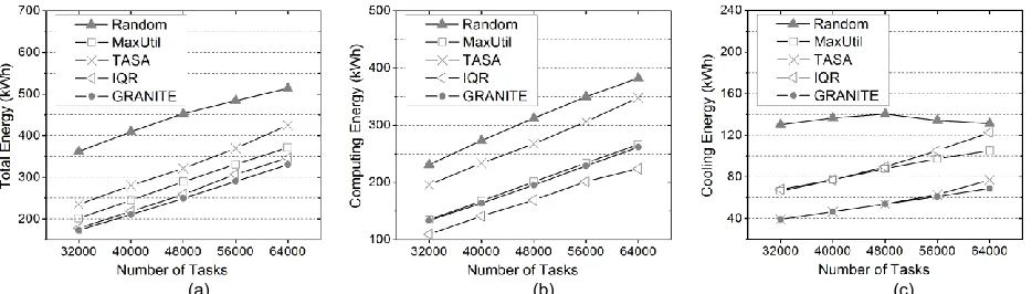
First we compare the energy consumption of each algo-rithm. We conduct experiments under different workload intensities and the results are presented in Fig 8. We ob-serve that GRANITE achieves the best energy efficiency in terms of total energy: 43.6% less than the worst (Random algorithm), 4.3% less than the second best (IQR), and 21.0% less than the average. To ascertain insight into the perfor-mance of each algorithm, we further analyze the details in TABLE2

EXPERIMENT PARAMETERS

Item Value

Datacenter

Number of racks 24

Number of servers each rack 15 (360 servers in total) Number of CRACs 4

Parameters of inlet

temperature model According to Section 4.2 Cooling update interval 300 seconds

Server

Heat capacity 340 [J/K] Thermal resistance 0.34 [K/W] Number of CPU cores 2-8 MIPS of each core 1,860, 2,660 CPU Power model Xeon3040, Xeon3075 CPU critical temperature 70°C

VM scheduler (VMM) Time shared

Workload

Parameters of tasks According to Section 4.1 Number of tasks

(each VM runs one task) 32,000-64,000 VCPU cores of each VM 1, 2 or 4

MIPS of each VCPU 500, 1000, 2,000, 2,500 Task scheduler Time shared

Simulator Simulation time 24 hours

[image:9.567.41.278.63.303.2] [image:9.567.38.277.76.304.2]

computing energy, cooling energy, system availability and reliabilities [33], respectively.

As illustrated in Fig 8(b), Random algorithm uses the most computing energy (48.1% more than others in aver-age), followed by TASA. Random algorithm does not take computing energy into consideration, which means an idle or inactive (e.g. sleep mode) server has the same chance to be the allocation target. This is contradictory to the basic idea of workload consolidation and leads to computing en-ergy waste. For TASA, due to its tendency of scheduling workloads to the server with the lowest CPU temperature, which may potentially be in sleep mod e or has been switched off. In other words, TASA balances tasks leading to much more active servers among the datacenter.

Fig. 9(a) shows the number of active servers during the experiment with 64,000 tasks. As illustrated, Random and TASA uses more active servers than the other algorithms. On the other hand, MaxUtil, IQR and GRANITE use less active servers, since (1) MaxUtil allocates workloads to the server with the maximum average utilization; (2) for IQR, it uses computing energy aware best-fit policy to initially pla ce virtual machines, allowing to intensify workloads in a smaller number of server; (3) for GRANITE, it selects a server with the minimum total power increase, and pre-fers to allocate the newly arrived workload to a non-idle server than activating a new server (described in Section 5.1). These three algorithms all consolidate workloads and lead to a satisfactory amount of computing energy.

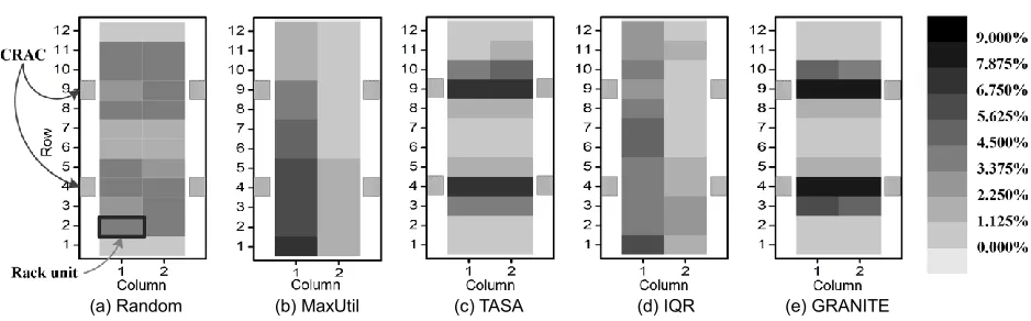
Fig 8(c) shows that Random, IQR and MaxUtil consume the most cooling energy, while GRANITE and TASA con-sume much less. To better understand the behind reason of the cooling efficiency, we demonstrate the average workload distribution among the datacenter with 64,000 tasks by Fig 10. There are 24 racks in total, placed in 2 col-umns that are described in the CFD modeling part (Section 4.2). The utilization is collected every 300 seconds during

the simulation and the averaged value is presented. We can observe that both TASA (Fig 10(c)) and GRAN-ITE (Fig 10(e)) allocate more tasks to racks nearer to the CRAC, which are more cooling efficient. This is because GRANITE - regardless whether it is within the initial place-ment stage or migration stage - attempts to select server without triggering temperature emergency to avoid cool-ing power increase. In other words, servers near a CRAC will more likely be the allocation candidate since they are comparatively cooler. Similar to GRANITE, TASA selects the coolest servers to allocate workloads and results in the similar workload distribution shown in Fig 10(c). For Ran-dom algorithm (Fig. 10(a)), utilization of the racks near CRACs is slightly higher than others. The algorithm ran-domly places VMs in the initial placement phase, and dy-namically migrates VM from hotter servers to cooler ones described in Section 5.2. Meanwhile, MaxUtil (Fig 10.(b)) and IQR (Fig 10.(d)) schedule workloads based on CPU utilization and are not temperature-aware. The former consolidates most workloads in the first group of racks, which are far from the CRACs, while the latter consoli-dates workloads to more racks which are not cooling effi-cient. The SAT using Random, IQR and MaxUtil will be lower compared to TASA and GRANITE, indicating higher CRAC usage cost.

Fig. 9(b) shows the results that are consistent with our analysis. In our experiment, each CRAC is dynamically ad-justed every 300 seconds according to datacenter tempera-ture. Results shown in Fig. 9(b) are the average SAT of four CRACs. We can learn that temperature-aware scheduling algorithms GRANITE and TASA can significantly increase the SAT and dramatically reduce cooling capacity.

Cloud providers must guarantee that the agreed ser-vices can be satisfied in terms of availability. Since we use dynamic migration, inevitably introducing potential SLA violation (10% during the migrations [32]). As shown in Fig.

[image:10.567.40.507.58.191.2]

(a) (b) (c)

Figure 8. Energy consumption of each algorithms: (a) total energy, (b) computing energy, (c) cooling energy.

TABLE3

AVAILABILITY OVERHEAD

Algorithm _Submitted Task _Finished Task _{Execution Time} Average SLA Violation _{Rate (%)}

Random

64,000

62,451 219.02 s 0.340

MaxUtil 62,825 218.59 s 0

TASA 62,825 218.59 s 0

IQR 62,792 218.82 s 0.013

GRANITE 62,700 218.94 s 0.170

TABLE4

HIGHEST CPUTEMPERATURE (COLLECTED EVERY 300S)

Algorithm _{Temperature (°C)} Average Highest Critical Temperature _{Violation (times)}

Random 71.54 1390

MaxUtil 69.32 212

TASA 65.68 120

IQR 69.42 335

[image:10.567.31.268.228.323.2] [image:10.567.290.534.244.324.2]

7, SLA violation rate is affected by the migration interval and migration threshold, which are defined as 300 seconds and 20%, respectively, as described above. The comparison of SLA violation rate between each algorithm is presented in Table 3. In our experiments, MaxUtil and TASA do not leverage live migration, so we assume that they can per-fectly meet the SLA. As illustrated, GRANITE suffers from higher SLA violation rate (0.17%), and requires more time (218.94 s) to finish tasks in average. However, the overhead in system availability remains satisfactory and acceptable.

Highest CPU temperature within the datacenter is

an-other important indicator of thermal management [12], [18] because (1) CRAC cooling efficiency are highly dependent on the temperature of the hottest server [34], [35], (2) sys-tem reliability [12], [33] will be significantly reduced if CPU violates its critical temperature frequently [26]. Fig. 9(c) shows the profiles of highest CPU temperature within the datacenter. Furthermore, Table 4 concludes the average highest temperature and the frequency of CPU critical tem-perature (70°C) violation. Since we observe that our algo-rithm rarely violates the critical temperature, we extend the experiment timespan to 10 days in order to get results with statistical significance. From the above results, we can observe that temperature-aware algorithms GRANITE and TASA achieve better result in most cases than non-temper-ature-aware algorithms MaxUtil, IQR and Random. Specif-ically, GRANITE reduce the probability of critical temper-ature violation by 99.2% in average, indicating a lower cooling requirement and higher hardware reliability.

7 R

ELATED

W

ORK

This section focuses on energy-aware management poli-cies designed for heterogeneous distributed systems such

as clusters and da tacenters. These policies comprises two categories: (1) software-level methods, such as task sched-uling and VM schedsched-uling; (2) hybrid methods, referred as mechanical design based methods [11], which further con-sider datacenter layout design, dynamic cooling, etc. Our method belongs to the latter category. This section intro-duces the representative work in each field, and a summa-rization is presented in Table 5 in terms of analysis scope, management methodology, evaluation, etc .

7.1 Software-Level Methods

Workload consolidation [5] is a common method to reduce computing energy and its main objectives is minimizing the number of active servers, assigning higher scheduling priority to servers with greater energy-efficiency, and avoidance of resource fragmentation [36]. Workload con-solidation is commonly modelled as a bin packing problem which has been proved to be NP-complete [15]. Work such as [7], [37] attempt to discover the optimal solution with linear program. However their method is confined only to comparatively small-scale datacenters. To address the NP-complete problem of scheduling, researchers tend to achieve the algorithm efficiency at cost of less solution ac-curacy. An intuitive algorithm called First-Fit Decreasing (FFD) is introduced [38] to address this problem, and it is further improved by [6] and [7]. Similarly, Lee and Zomaya [5] proposed two algorithms: ECTC and MaxUtil to consolidate tasks, with the former algorithm trying to maximize time period of tasks running in parallel with other tasks, and the latter trying to maximize average CPU utilization during execution. These above works mainly fo-cus on problem with 1-dimensional constraint (CPU avail-ability). To characterize the multi-dimensional resource

[image:11.567.53.520.59.189.2]

(a) (b) (c)

Figure 9. The profiles of (a) number of active servers, (b) supply air temperature, (c) highest CPU temperature within datacenter.

(a) Random (b) MaxUtil (c) TASA (d) IQR (e) GRANITE

[image:11.567.52.521.209.355.2]

usage states of servers, Li et al. [15] presented a multi-di-mensional space partition model, based on which they pro-pose a VM placement algorithm called EAGLE to balance the utilization of multi-dimensional resources and reduce the number of running servers. Furthermore, a concept termed “skewness”is introduced by [39] to measure the unevenness in the multi-dimensional resource utilization of a server. By minimizing skewness, they can combine dif-ferent types of workloads to reduce computing energy.

Apart from initial task/VM placement, scheduling sys-tems needs to dynamically adjust their execution for better energy efficiency. This becomes particularly important as the development of virtualization technology which al-lows for live migrations of VMs. Workload co nsolidation via VM migration can be modelled with linear integer pro-gramming formulation [36]. Beloglazov and Buyya [25] presented various of algorithms to deal with key problems in migrations such as selecting VMs to migrate out from overloaded server and selecting new placement for mi-grated VMs. [27] detailed their methodology in detecting overload and determing the best time for migration.

Mhedheb et al. [26] combined computing energy reduc-tion with CPU temperature management. Unfortunately, due to the incompleteness of models, they cannot explicitly connect CPU temperature with cooling capacity/status and propose any cooling energy aware scheduling algo-rithms. Moore et al. [8] proposed a system-level solution to control the heat generation through temperature-aware workload placement and reduce cooling energy. A sensor-based model to predict temperature distribution was pro-posed in [31], based on which Tang et al. [21] propro-posed an algorithm termed XInt to achieve cooling efficiency via

minimizing heat recirculation and peak inlet temperature. But the model proposed in [31] only considers a stable sta-tus of airflow and workload distribution. Such work is in-capable of capturing sudden fluctuation of workload and CRAC setting. Furthermore, the model only considers rack inlet temperature and does not model CPU temperature, which is a key indicator for thermal management [8], [12].

7.2 Hybrid Methods

CFD is a commonly deployed technique to model an entire datacenter with a specific layout [22], [23], [40]. Research in this field seeks to save energy and optimize datacenter operation at the hardware-level. Durand et al. [22] intro-duced a Proportional Integral Derivative (PID) algorithm to control the fan speed, combined with modeling servers and air conditioners. They consider the overall energy con-sumption in datacenters, and select the appropriate cool-ing temperature set point to reach the best compromise be-tween energy consumption of chillers and servers. Differ-ent airflow configurations within a datacDiffer-enter was studied by [10], who compared different airflow configurations and concluded that the vertical cooling schema “raised floor & ceiling return” was the most effective. Further studies show that datacenter racks with vertically placed servers attain enhanced cooling efficiency when vertical cooling schema is adopted [41].

Dynamic cooling is an effective means to enhance data-center energy efficiency towards minimizing cooling power draw. A proactive control approach is proposed in [11] that jointly optimizes the air conditioner compressor duty cycle and fan speed to reduce cooling cost and mini-mize the risk of equipment damage due to overheating. TABLE5

SUMMARIZATION OF REPRESENTATIVE MULTI-NODE ENERGY-AWARE MANAGEMENT POLICIES

Computing energy: , cooling energy: , SLA:  (response time, capacity requirement, etc.)

Author (first)

Policy Name Analysis Scope Components Scheduling Management Methodology Workload Model/ Source Performance Indicator Evaluation

Pakbaznia [19]

TA-DRP  Task Dynamic server retirement/employment Dynamic cooling Unknown Total energy TOMLAB/ MATLAB Lee [5]

MaxUtil, ECTC  Task Greedy based task consolidation Task migration Uniform distribution Gaussian distribution Computing energy Simulation Parolini [17]  Task Task scheduling and dynamic migration Constant arrival rates _Total energy _PUE TOMSYM/ _MATLAB Deng [42]  Task Solve Knapsack problem via dynamic _programming World Cup Web site _requests Throughput Real _measurement

Wang [12]

TASA, TASA-B  Task Temperature-aware task scheduling Datacenter of State Univer-sity of New York

CPU temperature

Job performance

Carbon emission Simulation Tang [21]

Xint  Task Task scheduling minimizing heat recirculation Unknown Inlet temperature Cooling energy Flovent Banerjee [19]

HTS  Task Task scheduling and dynamic cooling ASU datacenter Total energy Flovent Khosravi [14]

ECE  VM VM placement across multiple datacenter based on Best-Fit algorithm Hyper-Gamma distribution Carbon emission CloudSim Li [15]

EAGLE  VM Multi-dimensional resource constraint aware VM scheduling

Uniform distribution

Google cluster

Production system Computing energy Simulation Mhedheb [26]

ThaS  VM Temperature-aware VM scheduling 50 tasks Computing energy SLA violation CloudSim Beloglazov [25]

THR, IQR, MAD  VM Utilization-aware VM scheduling PlanetLab Computing energy SLA violation CloudSim Ferreto [7]  VM Consolidation via linear programming _{and heuristic based VM migration} _TU-berlin datacenter _{Google datacenter} _Number of used PMs _{Number of migrations Simulation}

Proposed approach

GRANITE  VM

Greedy based VM allocation

Dynamic VM migration,

Dynamic cooling

Google Cloud datacenter (25 million tasks)

Total energy

Job performance

CPU temperature

Fluent