http://www.scirp.org/journal/am ISSN Online: 2152-7393
ISSN Print: 2152-7385
DOI: 10.4236/am.2017.812128 Dec. 21, 2017 1795 Applied Mathematics
Chelyshkov-Tau Approach for Solving
Bagley-Torvik Equation
Mohamed El-Gamel, Mahmoud Abd-El-Hady, Magdy El-Azab
Department of Mathematical Sciences, Faculty of Engineering, Mansoura University, Mansoura, Egypt
Abstract
There are few numerical techniques available to solve the Bagley-Torvik equa-tion which occurs considerably frequently in various offshoots of applied ma-thematics and mechanics. In this paper, we show that Chelyshkov-tau method is a very effective tool in numerically solving this equation. To show the accu-racy and the efficiency of the method, several problems are implemented and the comparisons are given with other methods existing in the recent literature. The results of numerical tests confirm that Chelyshkov-tau method is superior to other existing ones and is highly accurate.
Keywords
Chelyshkov, Tau Method, Bagley-Torvik, Caputo Derivative, Residual Functions
1. Introduction
Recently, the fractional derivative has attracted a lot of attentions due to widely applied in various fields of physics and engineering. Fractional derivative is an excellent tool to describe memory and genetic characteristics of various materials and processes. Many phenomena in various fields of science and engineering such as control, porous media, electrochemistry, viscoelasticity, electromagnetic, etc. can be described by Fractional differential Equation (FDE). The evolution of effective and perfectly appropriate method for numerically solving FDEs has received great attention over the past years.
In this paper, we develop a new approach called Chelyshkov-tau method for solving Bagley-Torvik equation of the form
( )
( )3 2( )
( )
( )
[ ]
2 1 0 , 0,1
A u x′′ +A u x +A u x = f x x∈ (1) subject to the boundary conditions
How to cite this paper: El-Gamel, M., Abd-El-Hady, M. and El-Azab, M. (2017) Chelyshkov-Tau Approach for Solving Bagley-Torvik Equation. Applied Mathe-matics, 8, 1795-1807.
https://doi.org/10.4236/am.2017.812128
Received: October 26, 2017 Accepted: December 18, 2017 Published: December 21, 2017
Copyright © 2017 by authors and Scientific Research Publishing Inc. This work is licensed under the Creative Commons Attribution International License (CC BY 4.0).
http://creativecommons.org/licenses/by/4.0/
DOI: 10.4236/am.2017.812128 1796 Applied Mathematics
( )
( )
( )( )
10
0 1 , 0,1
j j
ij ij i
j
u u i
α β γ
=
+ = =
∑
(2)where A2 ≠0 represents mass of the thin rigid plate immersed in a Newtonian
fluid, A1 is constant depending on area of the thin rigid, viscosity and density
of fluid and A0 represents stiffness of the spring. f x
( )
is a given function.( )
u x represents motion of the rigid plate. The questions of existence and uniqueness of the solution to this initial value problem have been discussed in [1] [2], so there is no need to go into these matters here.
Several numerical and analytical methods of Equation (1) were considered by many authors, such as finite difference method [3], collocation method based on Müntz polynomials [4], Tau approximate [5], Adomian decomposition method
[6] [7], variational iteration method [8], the generalized block pulse operational matrix [9], homotopy perturbation method [10] [11], generalized differential transform method [12], Legendre-collocation method [13], Laplace transforms
[14], Fourier transforms [15], eigenvector expansion [16], fractional differential transform method [17] [18], the fractional iteration method [19], power series method [20], Bessel collocation method [21], wavelet [22] and the Haar wavelet method [23].
Orthogonal polynomials play an important role in mathematics as well as in applications in mathematical physics, engineering and computer science. Chelyshkov polynomials are the most recent set of orthogonal polynomials. Chelyshkov polynomials have become increasingly important in numerical analysis. The efficiency of the method has been officially established by many researchers [24] [25]. With these backgrounds, we extend Chelyshkov-tau method for solving Bagley-Torvik equation of Equation (1).
The efficiency and accuracy of the numerical scheme is assessed on specific test problems. The numerical outcomes indicate that the method yields highly accurate results. The numerical solutions are compared with analytical and other existing numerical solutions in the literature.
The paper is organized as follows. Section 2 preliminarily provides some definitions which are crucial to the following discussion. In Section 3 we apply Chelyshkov-tau method for solving the model equation. In Section 4, we present numerical examples to exhibit the accuracy and the efficiency of the present method. where the numerical results presented in this paper are computed by Matlab programming. The conclusion is presented in the final section.
2. Preliminaries
2.1. Basic Definitions of Fractional
In this section, we introduce the basic necessary definitions and primary facts of the fractional calculus theory which will be more used in this work [26] [27].
DOI: 10.4236/am.2017.812128 1797 Applied Mathematics
( )
( ) (
)
1( )
0 1
d
t
Jαψ t t s α ψ s s
α
−
= −
Γ
∫
Some characteristics of this operator are:
( )
( )
( )
( )
( )
( ) (
)
(
)
(
(
)
)(
)
(
)
0
, , , , 0
1
, 1
1
J t t J J t J t J J t J J t
J t s t s
α β α β α β β α
µ α µ
α
ψ ψ ψ ψ ψ ψ α β
µ µ α µ + + = = = ≥ Γ +
− = − > −
Γ + +
The Riemann-Liouville fractional derivative operator Dα is given by
( )
d(
( )
)
d
m m
D t J t
t
αψ −αψ
=
where m is an integer, provided that
m
− < ≤
1
α
m
.However, its derivative has Some drawbacks when we try to make a model for a real phenomenon using fractional differential equations. Therefore, we will provide a modified fractional differential operator Dα proposed by by Caputo
[28].
Definition 2. The Caputo derivative definition is defined as
( )
(
) (
)
1 ( )( )
0 1
d , 1 < ,
x m m
D t t s s s m m m
m
α
αψ ψ α
α
− −
= − − ≤ ∈
Γ −
∫
(3)Hence,
α
>
0
and m is the smallest integer greater than or equal to α. For the Caputo fractional derivative we have(
)
( )
( )
( )
( )
( )( )
(
)
(
)
(
)
1 00, is constant ,
,
0 ,
!
0 for ,
1
, for .
1
i m
i
i
D c c
D J t t
t s
J D t t
i D t t α α α α α α β β α ψ ψ
ψ ψ ψ
β α
β β α
β α − + = − = = − = − <
= Γ +
≥ Γ + −
∑
(4)It can be said when
α
∈
, the Caputo differential operator matches with the integer-order differential operator.For more details on fractional derivative definitions, theorems and its properties, you can see [26] [27].
2.2. Some Properties of Chelyshkov Polynomials
We first review some important concepts and basics of the Chelyshkov function and conclude useful results that are important to this paper. Recently, these polynomials have established by Chelyshkov in [29] [30] [31] [32] [33], which are orthogonal over the interval [0,1], and are explicitly defined by
( )
( )
0
1
1 , 0,1, ,
N j
i N k
Nj i
N j N j k
C x x j N
i N j
− + = − + + + = − = −
∑
(5)DOI: 10.4236/am.2017.812128 1798 Applied Mathematics
( ) (
)
1 1(
)
1 1 d
1 , 0,1, ,
! d
N j
N j N j
Nj j N j
C x x x j N
N j x x
− − + + + − = − = −
and the orthogonality condition of Chelyshkov polynomials [32] is
( )
( )
1
0
1
, for , , 0,1, , , 1
1 d
0, for .
Nj Nk
j k j k N N
j k C x C x x
j k = = + + + = ≠
∫
(6)Also it follows from this relation that
( )
1 1 0 0 1 d d 1 j NjC x x x x
j
= =
+
∫
∫
By using the Cauchy integral formula for derivative and the Rodrigues type representation, we can get the integral relation
( )
(
)
(
)
2
1
2 1 1
1 1 1 d 2π N j N j
Nj j N j
s s
C x s
i x s x
− + +
− +
+ Ω −
− =
−
∫
such that the point 1
s=x− . lies in closed curve Ω1.
Chelyshkov polynomials CNj
( )
x provide a natural way to solve, expand, andinterpret solutions. Actually, these polynomials can be expressed in terms of the Jacobi polynomials ( , )
k
Pα β by the following relation,
( )
(2 ,1)(
)
1 2 , 0,1, ,
j j Nj N j
C x =x P− − x j= N
Let function u x
( )
, square integrable in[ ]
0,1 , can be expressed in terms of Chelyshkov polynomials as( )
( )
( )
0
,
N
N j Nj
j
u x u x a C x
=
≅ =
∑
(7)where the coefficients aj are the unknown Chelyshkov coefficients and
, 0,1, ,
Nj
C j= N are Chelyshkov orthogonal polynomials of the degree N such that
N
≥
2
. Also,( )
( )
( )
0 0 ( ) , NN j Nj
j
N
N j Nj
j
u x a C x
u x a C x
=
=
′ = ′
′′ = ′′
∑
∑
(8)Then we can convert the solution expressed by (7) and its derivative (8) to matrix form
( )
( )
( )
( )
( )
( )
( )
2( )
( )
22 or d or d d or d
u x x u x C
x
u x u x C
x x
u x u x C
x = = ′ = ′ = ′′ = ′′ =
C A X A
C
A XM A
C
A XM A
(9)
where
[
a0, ,aN]
and( )
x CN0( )
x CN1( )
x CN2( )
x CNN( )
xτ
= =
A C
DOI: 10.4236/am.2017.812128 1799 Applied Mathematics
( ) ( )
2
1 1
0 1 0 0
0 0 2 0
1 , 0 0 0 0
0 0 0
0 0 0 0
N
N N
x x x
N + × + … … = = … …
X M
if N is odd,
1
0 0 0
0
2 1 2
0 0
1 0 1
2 1 2 1 2
0
1 2 1 0 1
2 1 1 2 1 1 2 1
1 1 1 1
N N
N
N N N N
N N
N N N N N
N N N N
N N N N N
N N N N
+ + − + − − = − − − − − + − + + − − − − C
( 1) ( 1) 1
N+ ×N+
if N is even,
1
0 0 0
0
2 1 2
0 0
1 0 1
2 1 2 1 2
0
1 2 1 0 1
2 1 1 2 1 1 2 1
1 1 1 1
N N
N
N N N N
N N
N N N N N
N N N N
N N N N N
N N N N
+ + − + − − = − − − − − + − + + − − − − C
( 1) ( 1) 1
N+ ×N+
Theorem 1. For CNj
( )
x defined in (5) then the finite series can be converted ( )3 2( )
( )3 2( )
( )3 2( )
0
N
N j Nj
j
u x u x a C x
=
≅ =
∑
into matrix form
( )3 2
( )
( )3 2u x
=
XD CA (10) where ( )
( )
( )
(
)
( ) ( ) 3 23 2 3 2
3 2
1 1
0 0 0 0 0 0
0 0 0 0 0 0
3
0 0 0 0 0
3 2
4
0 0 0 0 0
5 2
1
0 0 0 0 0
2 1
2 N N
x x N x N − − − + × + Γ Γ
Γ
=
Γ
Γ + … −
Γ
DOI: 10.4236/am.2017.812128 1800 Applied Mathematics
Proof. The proof is straightforward using Equation (4).
3. The Description of Chelyshkov Scheme
Let us seek the solution of (1) expressed in terms of Chelyshkov polynomials as
( )
( )
( )
0
. N
N n Nn
n
u x u x a C x
=
≅ =
∑
Replacing each terms of (1) with the corresponding approximations defined in (7), (8) and (10) and we obtain the following theorem.
Theorem 2. If the assumed approximate solution of the boundary-value problem (1)-(2) is (3), the discrete Chelyshkov-tau system for the determination of the unknown coefficients
{ }
0N n n
a = is given by
( )2
( )
( )3 2( )
( )
( )
2 1 0
0 0 0 0
N N N N
n Nn n Nn n Nn n Nn
n n n n
A a C x A a C x A a C x f C x
= = = =
+ + =
∑
∑
∑
∑
(12)Equation (12), which can be written in the matrix form
( )3 2 2
2 1 0
A XM CA+AXD CA+AXCA=XCF (13)
where
[
f0,f1, ,fN]
τ=
F
The residual RN
( )
x for Equation (13) can be written as( )
2 ( )3 22 1 0
N
R x =XAM CA+AD CA+ACA CF− (14)
As in a typical tau method [34] we generate N-1 linear equations by applying
( )
( )
1( )
( )
0, d 0, 1,2, , 1
N Nn N Nn
R x C x =
∫
R x C x x= n= N− (15) The boundary condition is derived from Equation (2) and matrices for conditions are( )
( )
1
0
0 j 1 j , 0,1
ij ij i
j
i
α β γ
=
+ = =
∑
X M CA X M CA (16)Equations (15) and (16) generate N+1 set of linear equations, respectively. These linear equations can be solved for unknown coefficients of the vector A. Consequently, u x
( )
given in Equation (7) can be calculated..4. Numerical Results
In this section, we apply the Chelyshkov-tau method to various problems which were collected from the open literature [13] [35] [36] [37] [38]. Our primary interest is to compare our method with other methods on the same problems. All computations were carried out using Matlab on a personal computer. In the examples, the maximum absolute error at points is taken as
Chelyshkov Exact Chelyshkov
E = u −u
DOI: 10.4236/am.2017.812128 1801 Applied Mathematics
( )
( )3 2( ) ( )
1, 0 1
u x′′ +u x +u x = +x < <x
subject to the boundary conditions
( )
0 1 and( )
1 2u = u =
whose exact solution is
1
u
= +
x
the approximate solution u x
( )
by the truncated Chelyshkov polynomial for 2N= is
( )
0 20( )
1 21( )
2 22( )
u x =a C x +a C x +a C x
Here, we have
( )3 2
3 2
3 0 0 0 1 0 0 0 0
4
12 4 0 , 0 0 2 , 0 0 0
π
10 5 1 0 0 0 0 0 x−
= − = =
−
C M D
2
1
3 5
1 ,
4 35
12
x x
= =
X F (17)
By applying Equation (15) We obtain
0 1 2
23 16 10 8 2 8 1
0
3 7 π a 3 7 π a 3 35 π a 3
+ − + + + − =
(18)
By applying Equation (16), we have
0
3a − =1 0 (19)
0 1 2 2 0
a − +a a − = (20) By solving Equations (18)-(20), we get
0 1 2
1 5 35
, ,
3 4 12
a = a = a =
Thus we can write
( )
2
2
2
10 12 3
1 5 35
5 4 1
3 4 12
x x
y x x x x
x
− +
= − + = +
which is the exact solution.
Example 2: [13] [35] [36] Consider the linear BVP
( )
( )3 2( )
( )
( )
2 1 0 , 0 1
A u x′′ +A u x +A u x = f x < <x
with initial conditions
( )
0 0 and( )
0 0DOI: 10.4236/am.2017.812128 1802 Applied Mathematics which is known to have analytical solution as
( )
(
) ( )
( )
( )
( )3 3
0
2 1
0 1
1 3 ,2 0
2 2 2 2 2
d
1 1
!
x
k k
k k
k k
u x G x f G x
A A
x E x
A k A A
τ τ τ
∞
+ + =
= −
−
= −
∫
∑
where ( ),
( )
k
Eλ µ u is the kth derivative of the Mittag-Leffler function with parameters
λ
andµ
given by( )
( )
(
)
(
)
,
0
!
, 0,1,2,
!
j k
j
j k y
E y k
j j k
λ µ λ λ µ
∞
=
+
= =
Γ + +
∑
and the G3
( )
x three-term Green’s equation. Let A2 =1, A1=A0=0.5 and( )
8 [image:8.595.211.538.536.731.2]f x = .
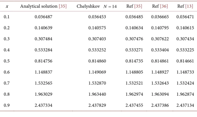
Table 1 exhibits a comparison between the exact, the results obtained by using Chelyshkov tau for N=14 with analogous results of Çenesiz et al. [35] for
underlying the generalized Taylor collocation method (GTCM) and Setia [36], who used second kind Chebyshev wavelet method (CWM) and with analogous results of El-Gamel and Abd El-Hady [13] for underlying Legendre-collocation method.
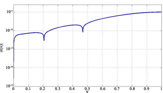
Figure 1 displays the estimated absolute error function for N=14 with the
present method.
Example 3: [13] [19] Now we turn to IVP
( )
( )3 2( ) ( )
8 3 2 37 1, 0 1
π
u′′ x +u x +u x = x+ x +x + < <x subject to the boundary conditions
( )
0 1 and( )
0 1u = u′ =
whose exact solution is
( )
3 1u x =x + +x
Table 1. Results for Example 2.
x Analytical solution [35] Chelyshkov N=14 Ref [35] Ref [36] Ref [13]
0.1 0.036487 0.036453 0.036485 0.036665 0.036471
0.2 0.140639 0.140575 0.140634 0.140795 0.140615
0.3 0.307484 0.307403 0.307476 0.307622 0.307434
0.4 0.533284 0.533252 0.533271 0.533404 0.533225
0.5 0.814756 0.814860 0.814735 0.814861 0.814661
0.6 1.148837 1.149069 1.148805 1.148927 1.148733
0.7 1.532565 1.532870 1.532521 1.532643 1.532424
0.8 1.963029 1.963440 1.962974 1.963094 1.962874
DOI: 10.4236/am.2017.812128 1803 Applied Mathematics
Figure 1. Error plot between analytical and Chelyshkov results for Example 2.
Table 2 exhibits a comparison between the results obtained by using Chelyshkov tau for
N
=
8
with analogous results of Mekkaoui and Hammouch[19] for underlying the variational iteration method (VIM), the fractional iteration method (FIM) and with analogous results of El-Gamel and Abd El-Hady [13] for underlying Legendre-collocation method.
Figure 2 displays the estimated absolute error function for N=8 with the
present method.
Example 4: [38] Consider the linear BVP
( )
8 ( )3 2( )
13( )
( )
, 0 1
17 51
u′′ x + u x + u x = f x < <x where
( )
1( )
( )
48 7
89250 π
f x p x x q x
x
= +
( )
4 3 216000 32480 21280 4746 149
p x = x − x + x − x+
and
( )
5 4 3 23250 9425 264880 448107 233262 34578
q x = x − x + x − x + x−
and subject to the boundary conditions
( )
0 0 and( )
1 0y = y =
whose exact solution is
( )
5 29 4 76 3 339 2 2710 25 250 125
y x =x − x + x − x + x
Table 3 exhibits a comparison between the absolute errors obtained by using Chelyshkov tau for
N
=
8
with analogous errors of Rehman and Ali Khan [38] for underlying Haar wavelets method.Figure 3 displays the estimated absolute error function for N=8 with the
DOI: 10.4236/am.2017.812128 1804 Applied Mathematics
[image:10.595.210.538.271.412.2]Figure 2. Error plot between analytical and Chelyshkov results for Example 3.
Figure 3. Error plot between analytical and Chelyshkov results for Example 4.
Table 2. Results for Example 3.
x Exact solution Chelyshkov tau N=8 Ref [19] Ref [13]
0.10 1.101000 1.101000 1.103763 1.101000
0.25 1.265625 1.265625 1.269040 1.265625
0.50 1.625000 1.625000 1.623997 1.625000
0.75 2.171875 2.171875 2.166900 2.171875
1.00 3.000000 3.000000 2.994988 3.000002
Table 3. Results for Example 4.
x Haar wavelets (N=256) [38] Chelyshkov tau (N=8)
0.1 6.49908E−7 5.92720E−14
0.2 6.35657E−7 1.18400E−13
0.3 3.71584E−7 1.77249E−13
0.4 9.48220E−7 2.35568E−13
0.5 1.59573E−6 2.17578E−13
0.6 1.05494E−6 2.92504E−13
0.7 6.34678E−7 3.82671E−13
0.8 1.88690E−6 3.82256E−13
[image:10.595.209.540.465.551.2] [image:10.595.210.538.582.738.2]DOI: 10.4236/am.2017.812128 1805 Applied Mathematics
5. Conclusion
In this paper, Chelyshkov operational matrix of fractional derivative has been derived. Our approach was based on the tau method. The proposed technique is easy to implement efficiently and yield accurate results. Moreover, only a small number of Chelyshkov polynomials is needed to obtain a satisfactory result. In addition, an interesting feature of this method is to find the analytical solution if the equation has an exact solution that is polynomial functions. Numerical examples are included and a comparison is made with an existing result.
References
[1] Luchko, Y. and Gorenflo, R. (1999) An Operational Method for Solving Fractional Differential Equations with the Caputo Derivatives. Acta Mathematica Vietnamica, 24, 207-233.
[2] Podlubny, I. (1999) Fractional Differential Equations. Academic Press, San Diego. [3] Meerschaert, T. and Tadjeran, C. (2006) Finite Difference Approximations for
Two-Sided Space-Fractional Partial Differential Equations. Applied Numerical Ma-thematics, 56, 80-90. https://doi.org/10.1016/j.apnum.2005.02.008
[4] Esmaeili, S. and Shamsia, M. and Luchko, Y. (2011) Numerical Solution of Frac-tional Differential Equations with a Collocation Method Based on Müntz Polyno-mials. Computers & Mathematics with Applications, 62, 918-929.
https://doi.org/10.1016/j.camwa.2011.04.023
[5] Vanani, S. and Aminataei, A. (2011) Tau Approximate Solution of Fractional Partial Differential Equations. Computers & Mathematics with Applications, 62, 1075-1083. https://doi.org/10.1016/j.camwa.2011.03.013
[6] Momani, S. and Al-Khaled, K. (2005) Numerical Solutions for Systems of Fractional Differential Equations by the Decomposition Method. Computers & Mathematics with Applications, 162, 1351-1365. https://doi.org/10.1016/j.amc.2004.03.014
[7] Ray, S. and Bera, R. (2005) Analytical Solution of the Bagley-Torvik Equation by Adomian Decomposition Method. Applied Mathematics and Computation, 168, 398-410. https://doi.org/10.1016/j.amc.2004.09.006
[8] Odibat, Z. and Momani, S. (2006) Application of Variational Iteration Method to Nonlinear Differential Equations of Fractional Order. International Journal of Non-linear Sciences and Numerical Simulation, 70, 27-34.
https://doi.org/10.1515/IJNSNS.2006.7.1.27
[9] Li, Y. and Sun, N. (2011) Numerical Solution of Fractional Differential Equations Using the Generalized Block Pulse Operational Matrix. Computers & Mathematics with Applications, 62, 1046-1054. https://doi.org/10.1016/j.camwa.2011.03.032
[10] Odibat, Z. (2008) Compact and Noncompact Structures for Nonlinear Fractional Evolution Equations. Physics Letters A, 372, 1219-1227.
https://doi.org/10.1016/j.physleta.2007.09.022
[11] Ganji, Z., Jafari, H. and Rostamian, M. (2008) Application of the Homotopy Per-turbation Method to Coupled System of Partial Differential Equations with Time Fractional Derivatives. Topological Methods in Nonlinear Analysis, 31, 341-348. [12] Odibat, Z. and Odibat, S. (2008) Generalized Differential Transform Method for
Linear Partial Differential Equations of Fractional Order. Applied Mathematics Letters, 31, 194-199. https://doi.org/10.1016/j.aml.2007.02.022
DOI: 10.4236/am.2017.812128 1806 Applied Mathematics Equation by Legendre-Collocation Method. SeMA Journal, 74, 371-383.
https://doi.org/10.1007/s40324-016-0089-6
[14] Uddin, M. and Ahmad S. (2017) On the Numerical Solution of Bagley-Torvik Equa-tion via the Laplace Transform. Tbilisi Mathematical Journal, 10, 279-284.
https://doi.org/10.1515/tmj-2017-0017
[15] Gaul, L., Klein, P. and Kemple, S. (1991) Damping Description Involving Fractional Operators. Mechanical Systems and Signal Processing, 5, 81-88.
https://doi.org/10.1016/0888-3270(91)90016-X
[16] Suarez, L., Shokooh, A. and Kemple, S. (1991) An Eigenvector Expansion Method for the Solution of Motion Containing Fractional Derivatives. Journal of Applied Mechanics, 64, 629-635. https://doi.org/10.1115/1.2788939
[17] Arikoglu, A. and Ozkol, I. (2009) Solution of Fractional Integro-Differential Equa-tions by Using Fractional Differential Transform Method. Chaos, Solitons & Frac-tals, 40, 521-529. https://doi.org/10.1016/j.chaos.2007.08.001
[18] Mekkaouii, T. and Hammouch, Z. (2012) Application of Generalized Differential Transform Method to Multi-Order Fractional Differential Equations. Mathematics in Computer Science, 39, 251-256.
[19] Mekkaouii, T. and Hammouch, Z. (2012) Approximate Analytical Solutions to the Bagley-Torvik Equation by the Fractional Iteration Method. Mathematics in Com-puter Science, 38, 251-256.
[20] Odibat, Z. and Shawagfeh, N. (2007) Generalized Taylor Formula. Applied Mathe-matics and Computation, 186, 286-293.https://doi.org/10.1016/j.amc.2006.07.102
[21] Yzba, S. and Shawagfeh, N. (2013) Numerical Solution of the Bagley-Torvik Equa-tion by the Bessel CollocaEqua-tion Method. Mathematical Methods in the Applied Sciences, 36, 300-312.https://doi.org/10.1002/mma.2588
[22] Wu, J.L. (2013) A Wavelet Operational Method for Solving Fractional Partial Diffe-rential Equations Numerically. Applied Mathematics and Computation, 214, 31-40.
https://doi.org/10.1016/j.amc.2009.03.066
[23] Lepik, H. (2009) Solving Fractional Integral Equations by the Haar Wavelet Me-thod. Applied Mathematics and Computation, 214, 468-678.
https://doi.org/10.1016/j.amc.2009.04.015
[24] Oguz, C. and Sezer, M. (2015) Chelyshkov Collocation Method for a Class of Mixed Functional Integro-Differential Equations. Applied Mathematics and Computation, 259, 943-954.https://doi.org/10.1016/j.amc.2015.03.024
[25] Oguz, C., Sezer, M. and Denk Oguz, A. (2015) Chelyshkov Collocation Approach to Solve the Systems of Linear Functional Differential Equations. NTMSCI, 3, 83-97. [26] Hilfer, R. (2000) Applications of Fractional Calculus in Physics. World Scientific
Publishing Company, Singapore.https://doi.org/10.1142/3779
[27] Diethelm, K. (1982) The Analysis of Fractional Differential Equations. Sprin-ger-Verlag, Berlin Heidelberg.
[28] Caputo, M. and Sezer, M. (1967) Linear Models of Dissipation Whose Q Is Almost Frequency Independent. Part II. Geophysical Journal of the Royal Astronomical So-ciety, 13, 529-539.https://doi.org/10.1111/j.1365-246X.1967.tb02303.x
[29] Chelyshkov, V. and Sezer, M. (1974) Stability of the Rest Position of the Inner Cy-linder in a Couette Flow. Fluid Dynamics, 6, 1003-1005.
DOI: 10.4236/am.2017.812128 1807 Applied Mathematics [31] Chelyshkov, V. (1986) Using the Method of Integration with Respect to a Small Pa-rameter for Calculating a Laminar Boundary Layer on a Cylinder. USSR Computa-tional Mathematics and Mathematical Physics, 26, 94-96.
https://doi.org/10.1016/0041-5553(86)90047-9
[32] Chelyshkov, V. (2006) Alternative Orthogonal Polynomials and Quadratures. ETNA, 25, 17-26.
[33] Chelyshkov, V. (1994) A Variant of Spectral Method in the Theory of Hydrody-namic Stability. Hydromech, 68, 105-109.
[34] Canuto, C., Hussaini, M. and Quarteroni, A. (1988) Spectral Method in Fluid Dy-namic. Prentice-HLL, Englewood Cliffs.https://doi.org/10.1007/978-3-642-84108-8
[35] Çenesiz, Y., Keskin, Y. and Kurnaz, A. (2010) The Solution of the Bagley-Torvik Equation with the Generalized Taylor Collocation Method. Journal of the Franklin Institute, 347, 452-466.https://doi.org/10.1016/j.jfranklin.2009.10.007
[36] Setia, A., Liu, Y. and Vatsala, A. (2014) The Solution of the Bagley-Torvik Equation by Using Second Kind Chebyshev Wavelet. 11th International Conference on In-formation Technology.
[37] Bagly, R. and Torvik, P. (1984) On the Appearance of the Fractionl Derivative in the Behavior of Real Materials. Journal of Applied Mechanics, 51, 294-298.
https://doi.org/10.1115/1.3167615