A mixed integer linear programming approach to forest utilisation management problems

TO FOREST UTILISATION MANAGEMENT PROBLEMS

A thesis

submitted in partial 1 lment of the requirements for the Degree

of

Doctor of Philosophy in Forestry in the

University of Canterbury by

L. R. Broad

ACKNOWLEDGEMENTS

Especial thanks to Professor McKelvey for providing both encouragement and leadership, skills used so

constructively to effect the running of t,he Forestry School during the period he held the chair. Thanks are also due to Dr. Whyte, my supervisor, without whose help this study would neither have been instigated nor completed, his assistance and advice are gratefully acknowledged; to Dr. George

(Operations Research) for making time available for discussion. Assistance was so given by Dr. Walker in allowing me to

read his yet unpublished book titled "How to recognise educational paradigms".

Thanks are due to Dr. Robinson (Mathematics) for his work on multi-stage processes which served as the basis for Chapter 4; to Professor Deely (Stati cs) for a rhapsodical

introduction to decision theory (a subject that engenders indecision), and his colleagues Drs Chacko, Smith and Wood for presenting the rudiments of statistical theory in a thoroughly understandable way, i.e., statistics without sadistics.

Many people deserve mention for their tolerance and forbearance amongst whom are my typist, Mary Kinniard, and flatmates. The last bracket is inclusive of Master Ritchie whose culinary skills with the genus Cuaurbita must be mentioned.

ABSTRACT

The research reported here concerns the use of

mathematical programming techniques to model resource flows in a system comprising industrial forests and subsequent wood processing and marketing activities. A review is made initially of methods to delineate management alternatives in industrial forests through formulating and solving linear programs. Linear programming techniques used to represent the associated Forest Management Problem (FMP) are discussed and solution methods analysed. The use of linear programming and mixed integer linear programming to represent resource flows in a problem where, in addition to forest management activities, the utilisation and marketing of wood based resources are also considered is explored in considerably more depth. Previous research on this latter class of

problem, termed a Forest Utilisation Management Problem (FUMP), has been limited. Forest utilisation management problems

may be characterised by the joint occurrence of standard Operations Research problems such as those of location, resource allocation, budget measures, and fixed charge

specification. Mixed integer linear programming techniques appeared to provide a viable means to resolving FUMPs that pose non-convex programming problems. The possibility of redundancy in FUMPs is considered, and a technique to assist in preventing i t is presented. The implications of redundancy to problem formulation are made apparent.

generation, and report writing. Recommendations concerning formulation and solution of FUMPs are made. Conclusions drawn relate to the asibility of representing FUMPs as a class of mathematical program.

Key Words Forest planning model, wood utilisation,

Chapter

1

2

CONTENTS

Page

Dedication

Acknowledgements

Abstract

STUDY OUTLINE

1.1 Study objectives

1.2 Outline of chapter contents in thesis

FOREST REGULATORY MECHANISMS

2.1 Stand level management mechanisms 2.2 Forest level management mechanisms

i

ii

i i i

1 7 8

10 11 16 2.2.1 Representation of management units 18 2.2.2 Single crop-type structural 19

constraints

2.2.3 Single crop-type regulatory 22 constraints

2.2.4 Multiple crop-type structural 23 constraints

2.2.5 Multiple crop-type regulatory 29 constraints

2.3 Bounding and smoothing regulatory 31 constraints

2.4 Solution techniques for forest management 37 problems

2.4.1 Standard simplex methods 38 2.4.2 Decomposition methods, model I 39 2.4.3 Decomposition methods, model II 41 2.4.4 Dual variable estimation 42

Chapter

3 TRANSPORT UTILISATION AND MARKETING

3.1 Description and measurement of resource flows

3.2 The transportation mechanism

3.3 Introductory regulatory mechanisms 3.3.1 Non-convex interpolating binary

mechanism

3.3.1.1 The location problem 3.3.1.2 The resource allocation

problem

3.3.1.3 The budgeting problem 3.3.1.4 The fixed charge problem 3.3.2 Non-convex non-interpolating

binary mechanism 3.3.3 Convex mechanisms

3.3.3.1 Constant returns to sca 3.3.3.2 Diminishing returns to

scale 3.4 Marketing mechanisms

3.5 Structural considerations for FUMPs 3.5.1 Bender's algorithm

3.5.2 Processing networks

Page

48

53

58 59 62

64 65

71 74 76

78 80

84

88

88 91

4 SPATIAL AND TEMPORAL EFFECTS OF ROUNDWOOD

AVAILABILITY 94

4.1 The resource digraph approach 96 4.2 The manufacturing digraph approach 103

4.3 The generator set approach 115

Chap bel'

5

6

Page

COMPUTATIONAL EXPERIENCE 121

5.1 Description of test problem 122

5.1.1 Data base requirements 129

5.1.2 Report writer output description 144

5.1.3 Singularity report 150

5.2 Matrix generation: development and validation

153

5.2.1 Observations on matrix generators 156 5.2.2 Observations on report writers 160 5.3 Restricted answers from planning models 162

5.3.1 Model aggregation 163

5.3.2 Estimation errors 164

5.3.3 Stochastic elements 165

5.3.4 Cost considerations 166

5.3.5 Uncertainty in economic efficiency 167 measures

DISCUSSION AND CONCLUSIONS 169

6.1 Discussion 169

6.2 Study conclusions and recommendations 179

REFERENCES 183

LIST OF FIGURES

Figure Page

2.1 Alternatives for a model I management unit 20 2.2 Digraph showing model I management alternatives 25 2.3 Digraph showing model II management alternatives 27 2.4 A resource lower bound envelope 34 2.5 A resource upper bound envelope 36

3.1 General flow digraph 51

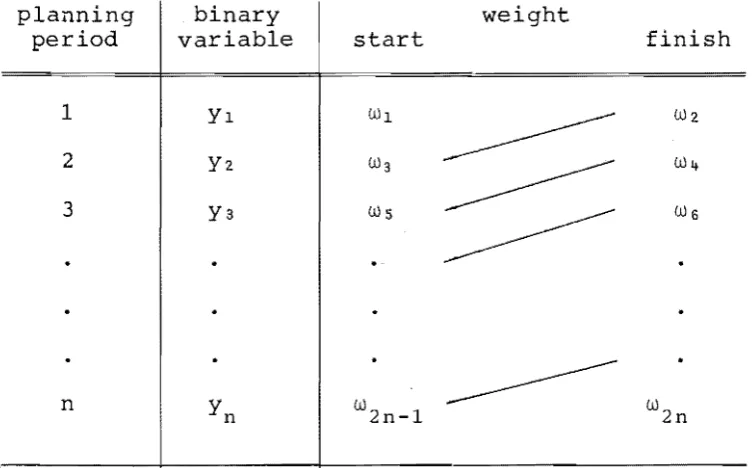
3.2 Control of continuous weights 63

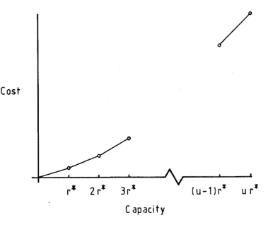
3.3 Introduction cost vs capacity 81

3.4 Process types in a processing network 92 4.1 Resource digraph for a four-stage process 97 4.2 Manufacturing digraph representing a three- 104

st process

4.3 Resource digraph representing a three-stage 106

5.1

5.2

process

General flow digraph illustrating option on continued log sales, and expansion of

processing and marketing options

Generalised growth curves in even-aged stands

127

134

5.3 Cutting patterns for two type I management units 137 5.4 Generalised roundwood conversion subdigraph

modelled as a three-stage conversion process

LIST OF TABLES

Table Page

2.1 Tableau of crop-type revenues and costs

13

3.1

3.2 Tabulation of repayment sequences 73

CHAPTER 1

STUDY OUTLINE

To specify a single raison d'etre for all integrated forest products companies, other than economical survival, is difficult in that such companies may differ markedly from each other in their management policies. what can be said, however, is that all integrated forest products companies face in common major problems of resource allocation in their operational management, and that these problems arise

naturally as part of the company's activities. Problems encountered involve scheduling

1. Roundwood harvested from forest estates and other supply sources regulated by the company;

2. Processing activities where utilisation of roundwood takes place;

3. Product sales at markets;

4. Transportation of roundwood or roundwood based products; and

5. Finance, energy and manpower requirements.

Each of these problems is basic to the activities of an integrated forest products company, and as discussed

later in this chapter, solutions appropriate to all of these problems are not usually obtained by attempting solutions to individual problems.

the management problems posed by integrating these two aspects. If FUMPs are considered at regional or ional level, their regional or sector planning problems would rise (Baird and Whyte, 1982; Whyte, 1984). Related to a Forest Utilisation Management Problem is the notion of a Forest Management Problem (FMP). FMPs are concerned with the growing of forest resources only, and with the management problems posed therein. Explicit consideration is not given to uti sat ion alternatives. However, implicit consideration may be given in that, for example, a management decision

may be to determine which roundwood resources to produce; these resources being strongly linked to their intended use within some form of utilisation. Typically, mechanisms to regulate st growth can be considered to arise from FMPs. The FMPs of interest to this study will be those that give rise to linear programming formulations (Johnson and Scheurman,1977). To facilitate discussion the distinction between an FMP and the forms of representation i t gives rise to will often be dropped, similarly for FUMPs.

To conduct an examination of the resource allocation problems of a FUMP, note the distinct notions of

1. A production process (often abbreviated to process); and 2. A processing centre.

As used within this study, a production process is defined as being a process involving the conversion of input resources to output resourceS1 inputs must be consumed in order that outputs be produced. A processing centre is

Example 1.1

Highly regulated forest stands (or crops) such as those found in commercial forest enterprises are usually

even-aged and homogeneous in such other attributes as species composition, silvicultural tending, and harvesting method. The growth of such a stand over a number of time periods can

be considered to be a production process (management

alternative) where product formation (roundwood produced) is assumed to be made available by harvest of the stand during a time period. Such a process starts with afforestation or reforestation and ends with harvesting. For each process representing a specified stand, the process is characterised by a set of attributes that distinguish i t from other processes. Among such attributes might be times to start and finish the process and the composition of wood resources obtained from the process. Each area available for management may have a number of stands proposed for it, each characterised by a different management process. Forests can be considered as aggregations of such areas. The spatial and temporal

distribution of harvest volume is obtained by coordinating the harvest volumes of stands within the forest. Thus, a forest can be regarded as an aggregation of processes into a

processing centre. ~~

The introductions of the notions of production

processes and processing centres allows the resource allocation problems within an FUMP to be examined from the view of

controlling activities within and between processing centres. Processing centres play a central role in "balancing" resources

in FUMPs, in that

with resource availability.

2. If resources are transferred between processing centres/ then resource conservation is ensured in the transfer.

As an example of point 1/ the production of roundwood by processes within a centre must be done in a manner consist-ent with the availability of resources necessary for

production. These resources may include land/ labour/ and monies expended or roundwood production. This represents the balancing of resources within a processing centre.

This notion of balancing resources within and between processing centres shall be termed integration. Subsequently in this study/ the expression integration of processing centres/

or simply integration will be used.

The integration of processing centres has implications as to the possibility of decentralised planning at processing centres. This arises because the balancing/ by processing centres/ of shared and transferred resources implies that separate decisions cannot be made for each processing centre, then truly decentralised planning cannot exist. Thus/ i t is only by integration of processing centres that overall economic efficiencies can be pursued (Lasdon, 1970).

Processing centres can be integrated in various ways. These methods usually give consideration to quantit sand/or prices of resources transferred. At the outset/ then/ the writer must emphasise that this study is concerned with methods of integration that are efficient in some well-defined economic sense. It is not concerned with methods of integration

complex". In New Zealand, the link between the size of a forest grower and the incorporation of equity notions into

st management is very strong.

The functioning of some mathematical programming algorithms that are used to identify optimal levels of

economic efficiency for integrated processing centres can be explained in terms of successive specification of prices of shared resources until an optimality condition is satisfied

(Dantzig and Wolfe, 1960). The most simple form of integrat-ion and the one most commonly practised is that specifying requests or orders between processing centres. In this way, production and consumption levels for shared resources

can be matched. As a result each processing centre is set a reasonably well-defined task as to what i t must do.

As can be imagined, the number of foe ble ways of obtaining integration between processing centres immense. The question then arises, Ills i t possible from among the many ways of integration to select better ways?1I Selection may be achieved through making comparisons between alternative methods of integration and then making a better selection. In practice, this may be done by adopting a well-defined economic efficiency measure so that higher measures of efficiency are associated with better ways of integration.

Consideration will now be given as to why a mechanism that specifies integration as a requirement, and methodically searches for gains in economic efficiency is important in relation to FUMPs. The two extremes in the construction of planning models to represent the activities within a FUMP are simulation techniques and optimis"ation techniques.

that a scenario is specified and the model is run to set out in detail the activities of that scenario. Simulation techniques are usually computationally faci and cost little to run provided the detail demanded of them is not excessive. The limitations of these techniques, however, is that better scenarios may exist but may remain undetected in that they have not been explicitly formulated for examination.

Alternatively, constrained optimisation techniques allow integration of processing centres through constraint

specification, and the pursuit of economic efficiency through the generation of a sequence of feasible solutions with

corresponding monotonic objective function values. The procedure ends when no method of integration can be found that is better than the incumbent. Conceptually, successful termination should always occur when the problem has been formulated correctly.

The possibility of advantage to be gained through application of optimisation techniques is what makes them appropriate vehicles to examine FUMPs. For this reason, the forest planning models developed and discussed in this study are largely optimisation based.

Mathematical programs representing FUMPs can become large (Clutter et al., 1983), so the need for representations with 1e resolution techniques is obvious. Because

resolved by the inclusion of integer variables into a model. For these problems, a Mixed Integer Linear Program (MILP) suffices for the purposes of representation (Murty, 1976).

To facilitate the examination of integration and

efficiency within FUMPs, the study objectives in section 1.1 were outlined. These objectives directed the examination of FUMPs towards the related problem aspects of formulation, generation, solution and report writing. section 1.2 contains a chapter summary and shows how this enquiry was pursued in succeeding chapters.

1.1 STUDY OBJECTIVES

The objectives of this study are set out in 1 through 4 below.

1. To formulate, using Linear Programming (LP) or Mixed

Integer Linear programming (MILP), a system characterising resource flows for a generalised Forest Utilisation

Management Problem.

2. To identify means by which the classes of program

representing Forest Utilisation Management Problems may be generated and solved.

3. To evaluate, for various formulations characterising components of Forest Utilisation Management Problems, features such as model generation, ease of solution, and information gained.

4. To examine critically the feasibility, the benefits, the difficulties and the drawbacks of using mathematical programming techniques to model Forest Utilisation

The first of these objectives requires that the mechanisms that permit integration between and within

processing centres be developed. Implicit in the statement of this objective is that the relationship between the

integrative mechanisms and production models at processing centres be made clear.

The second objective leads to an examination of solution mechanisms in chapter 3 and the specification of a test problem in chapter 5.

The third objective leads to the identification in chapter 2, and the development in chapter 3 of various formulations of model components.

Finally, the fourth objective leads to a discussion in chapter 5 on the efficacy of using mathematical programming techniques for forest planning problems generally and in

particular to the forest/utilisation planning problem.

1.2 OUTLINE OF CHAPTER CONTENTS IN THESIS

The remaining chapters in this study are described by content as follows.

In chapter 2, stand and forest level management

mechanisms as means to govern resource flows (roundwood) from forests are examined. This is given in relation to linear programming representations of FMPs. Solution techniques for the LPs that arise are discussed.

Chapter 3 is concerned with the governing of resource flows that occur within the utilisation phase of a FUMP.

to structural aspects of FUMPs are also considered. In chapter 4, methods that enable the possible prevention of redundancy in parts of an FUMP are examined

(specifically, the prevention of redundancy in production models involving multistage processes is examined), the

potential redundancy arising through resource unavailability. This has implications for matrix generation and may possibly allow the removal of integer variables from MILPs representing FUMPs.

Chapter 5 gives the discussion of a test problem used to test model components and procedures developed in chapters 2,3 and 4. In addition, general observations on matrix

CHAPTER 2

FOREST REGULATORY MECHANISMS

Solutions to the Forest Utilisation Management Problem (FUMP) require that the pattern of' forest resources to be harvested over time be established and that the accompanying forest management activities be specified. In short, this involves forest level planning and the preparation of a harvest schedule.

Examined and extended in this chapter are some of the methods used in preparation of forest schedules. Collectively, these methods allow solution to a forest management problem. The approach initially is historical, concerned firstly with

stand-level management techniques, then with the regulatory and structural aspects of forest-level planning mechanisms formulated as mathematical programs.

An outline of the sections is as follows: section 2.1 presents an historical outline of stand level management

2.1 STAND-LEVEL MANAGEMENT MECHANISMS

Stand-level management considers a forest as a number of stands, each of which is homogeneous for management purposes, usually age, species, and productive capacity. Each stand

is then managed individually, using some criteria of

efficiency, either economic or productive, to determine what constitutes the ~best~ stand management policy. The use

oC

When stands are considered as homogeneous in age, spec s, and productive capacity and the question is to determine what rotation length will maximise the volume produced over an infinite time horizon, then one can easily show that, if successive rotations for the stand have the rotation age of maximum mean annual increment (MAl), then

the volume production per unit area will be maximised (Clutter et al., 1983). The use of any other rotation age will result in a lower average production rate (MAl) for each rotation, which will lower the total volume produced over an infinite

time horizon. Appendix 2.1 documents some of the well known important relationships concerning mean annual increment

(MAl) and current annual increment (CAl).

In the situation of determining which rotation age to use for a single crop type, Clutter et aZ., (1983) cite the following decision criterion to maximise volume:

where

max [MAlt] t

t is the stand age Y

t is the volume per unit area at age t, and MAI

t is the mean annual increment at age t.

In choosing both crop-type and rotation age Clutter

et al., (op. t.) use the criterion.

( 2 .2)

where

t is

k the stand age of crop type k

Y is the volume per unit

tk

at age t for crop type k, and

MAlt is the mean annual increment at time t for crop type k. k

These decision criteria assume an infinite planning horizon and also assume that any crop type, once initially established, will be reafforested after each harvest. Both these assumptions are usually relaxed when considering forest level management techniques, in that both a finite time

horizon and transferral of areas between crop-types are permissible.

Volumetric decision criteria such as (2.1) and (2.2) seldom suffice as adequate criteria for selecting stand-level management methods, in that most management objectives are

ultimately economic in nature. Instead, economic criteria that account for the time value of money and the flow of costs and returns that may occur over a rotation or planning horizon are more attractive as decision criteria. Those criteria that consider the flow of costs and returns over a rotation all require as input a statement of costs and returns for the proposed rotation as in Table 2.1.

Those methods using a planning period require a

sequence of net revenues, discounting ing adopted because i t incorporates the time value of money and allows comparison of projects that may terminate at different points in time.

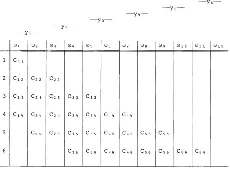
Table 2.1 Tableau of Crop-Type Revenues and Costs Tabulated for a specified crop-type are

the revenue and cost flows during a rotation of length n years.

t revenue @ _{t cost} @ _t

0 ro Co

1 rl Cl

2 rz Cz

n r c

n n

where

'f~. _{is the revenue per unit area in year i}

1.

C. is the cost per unit area in year i . 1.

One common rotation-based economic measure is land expectation value (LEV), which considers the present value of an infinite sequence of rotations, each having the

where LEV t

r.

t t - '

L

j=o J J

(1+i) t_1 (2 • 3)

is the land expectation value in monetary units for a rotation length of time t, (this is also known as soil expectation value);

is the revenue associated with time j of the rotation; is the cost associated with time j of the rotation; is the rotation length in time units1 i and

is the discount rate per unit time.

The following measures can either be rotation or planning-horizon based~ they are defined by (2.4) and (2.5) to be the sum of the sequence of discounted or compounded net revenues respectively.

where

t

NPV =

t

j=O

(r.-c.)

J J

(1+i)j

t (r -c )

NFV

=

L

..

NPV is the net present value NFV is the net future value

r. is the revenue per unit

J

in monetary in monetary area in time c. is the cost per unit area in time j •

J

(2 • 4)

(2. 5)

units, units,

j, and

In the general case of choosing both crop-type and rotation age, the following economic decision criterion can be formulated given measure (2.3)

1 A distinction is sometimes made between rotation age and rotation

max

k [ max

[LEVt

1]

- t k

k

(2 • 6)

However, decision criteria similar to the measures

(2.4) and (2.5) must be applied with care in that they include a fraction of a rotation if the measures are applied to a

planning horizon that is not an integral number of rotation lengths.

The use of an economic decision measure implies that a ranking can be stated as to the relative desirability of proposed rotations. However, in general, the rankings derived from employing differing economic measures will be different. Equations (2.3) and (2.4) each suggest a ranking relation, with ties being broken arbitrarily.

relations are as follows:

then choose crop-type k with rotation length t; if NPV

tk

then choose crop-type k with rotation length t.

These

Each of these ranking relations allows the construction of the preferred ordering of the rotations proposed for a

stand. However, the preferred orderings, or rankings, are not necessarily the same when different ranking relations are used. Given the above ranking relations, the following is possible:

and

Thus, the sets of available economic measures are not necessarily consistent in their rankings, and debate surrounds the choice of measures. Forest level management is obtained by the integration of stand-level management. The inability to generate consistent rankings under all

measures carries over to the forest-level management problem, and also to the forest utilisation management problem.

2.2 FOREST LEVEL MANAGEMENT MECHANISMS

Concepts from stand level planning techniques play an important part in forest-level planning techniques because the latter can be considered to involve joint management of the former. The joint management or integration being

required in order to satisfy production smoothing requirements. The smoothing considerations mean that decisions can no

longer be made independently for each stand and that decision making techniques that are capable of integrating the production

from stands so as to meet the smoothing requirements must also be used.

target forest concepts played an important role in the preparation of cutting schedules. For examp , a "normal forest" was considered to be an idealised structure whose attainment and subsequent maintenance was considered to constitute good management practice. Such considerations are, at the time of writing, regarded as anachronistic. However, target forest concepts s t i l l remain in forest planning, with "fully regulated forestsll (cited in Clutter

et al., 1983) and "equivalent normal forests" (Allison et al.,

1979) having arisen to describe what are considered suitable target situations. Japanese forest planners still give

strong consideration to target forest concepts (Suzuki, 1984; Choi and Nagumo, 1984), and mathematical programs designed to attain a specified target forest structure from a given initial forest structure have been formulated (Choi and Nagumo, op. cit.).

Most forest-level management techniques currently allow what Clutter et at. (1983) term "the intelligent management of imbalanced forest structures". Loosely speaking, these can be considered to be a relaxation of target forest concepts, where the allowed targets are not so rigorously defined. The motivation for the relaxation is that stable forest communities, other than those based on target forest concepts, can exist and moreover these

communities may be attractive economically.

This section details mechanisms used in forest-level management that may be formulated using mathematical

representations; subsection 2.2.3 introduces the regulatory constraints to achieve integration of management units; and, regulatory constraints necessary to deal with mUltiple crop-types.

2.2.1 Representation of Management Units

Assuming forest level management is concerned with management of stands, each of which is homogeneous with

respect to crop-type, age class, and productive capacity, then forests with such stands can be partitioned into

crop-type age classes because each such stand can be located to only one crop-type age class. Different stands belong to different crop-type age classes.

The partition of an area into its constituent crop-type age classes can change over time because forest growth is characterised by the transfer of areas between age classes and possibly crop-types over time as areas are harvested and reafforested . The current definitions for a management

. t 2

un1 , model I and model II (Johnson and Scheurman, 1977) are defined in relation to the area partitions induced by crop-type age classes. They differ in that model II

formulations consider how this partition may change over time. A model I formulation does not use area transfers

between crop-types as part its definition. Instead, i t uses the crop-type age class area partition induced in the initial planning (model) period to define management units. That is, each crop-type age class having a non-zero area in the initial planning period constitutes a management unit. A model II formulation, on the other hand uses the area partition induced in each planning period to define

2. Ware and Clutter (1971) term such devices cutting units. In this study,

management units. Thus implicitly incorporating the area transferred3 _{between age classes and crop~types as part of}

the definition.

In a model I formulation, strategies are proposed for a management unit, whereas for a model II formulation, the strategies proposed determine the management units that may arise during the planning horizon. Model I management units always have an area associated with them, whereas

for those model II units formed during the planning horizons, this is not necessarily so.

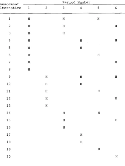
Figure 2.1 shows the management alternatives proposed for a single model I management unit. These same alter-natives would represent seven management units in a model II formulationj the initial management unit established

at least two periods before period 1, and the six management units arising from harvest of the initial crop-type in

periods 1 through 6, or from harvest of a subsequent crop-type in periods 3 through 6.

2.2.2 Single Crop-Type Structural Constraints

The constraints used to express conservation of

area for management units that arise in a model I or model II formulation are termed structural constraints, whereas those constraints that integrate the flow of resources from manage-ment units shall be termed regulatory. It is not surprising that differing sets of structural constraints arise for Model I

3

crop-type age class transfers between periods can occur as follows:

a. No harvest occurs and the subsequent age class is entered the subsequent period;

b. A harvest occurs with reforestation of the same crop-type, and the first age class is entered in the subsequent period;

Management

alternative 1

1 H

2 H

3 H

4 H

5 H

6 H

7 H

8 H

9 10 11 12 13 14 15 16 17 18 19 20

Figure 2.1

Period Number

2 3 4 5 6

H H

H H

H

H H

H

H

H

H H H

H H

H H

H H

H

H H

H H

H

H

H

H

H

Alternatives for a model I management unit.

The management unit arises from a crop-type age class containing harvestable volume in the initial planning period. The minimum rotation

length is two periods, H denotes the harvest/ reafforestation of the same crop-type.

and model II management units since the units are defined in different ways in terms of the area partitions induced by the crop-type age classes.

In the case of a single crop-type, Johnson and

Scheurman (1977) define the model I and model II structured constraints respectively as equations (2.7) and (2.8)

RQ,

where

where

~ XQ,

=

q::::1 q

(2.7)

Q, :::: 1, . . . ,U

are the units of area of management unit Q, assigned management alternative q,

are the units of area of management unit Q"

U is the number of management units, and

RQ, is the number of management alternatives for management unit Q,.

k

N

~

j =1 X . .

l.J

N

~

jk j+z

+

l.N

+

~

i = - M , . . . ,O

j

=

Vi

(2 • 8)

X.

l.j Vj

X •• (x . k) are the units of area reforested in period i (period j)

l.J J followed by harvest/reforestation in period j (period k) i

WiN(W

jN) are the units of area reforested in period i (period j) _{and left as part of the ending inventory in period N;}

A. l.

N

M

are the units of area present in period one that were either afforested or reforested in period i, with each A being a constant at the beginning of the planning horizon (period 1) i

is the number of periods in the planning horizon; is the number of periods before period zero in which the oldest age class in period one was afforested or reforested;

2.2.3 Single Crop Type Regulatory Constraints

Constraints to integrate the flow of resources from management units, the so called regulatory constraints, may

include harvest area; harvest volume; residual area; residual volume; and area transfer constraints. These can all be formulated as linear combinations of the activities in a model I or model II formulation, and they by no means exhaust the set of meaningful combinations that can be

formed for regulatory purposes (Garcia, 1984). Historically, foresters have been concerned with harvest volume or harvest area constraints as the ch f regulatory mechanisms.

Johnson and Scheurman (1977) present (2.9) as harvest

volume constraints, which are smoothing but not bounding, in that they smooth the flow of harvest volume between periods but do not bound i t explicitly at each period.

where

where

Model I harvest volume expression

h.

J

Vn .

x.qJ

u

J = _,Q,=1

I

L

V n .Xll

x.qJ x.q

is the total harvest volume in period j,

is the volume per unit area harvested in period j, from management unit Q, under management alternative q.

Model II harvest volume expression

h.

J

V. 'k _1J

h. =

J N

L

I

N

v ..

+

I

v.,

1 J 1 i = -M 1 J 1

is the total harvest volume in period j; and

is the volume per unit area ar1s1ng in period j with afforestation or reafforestation in period i with clear felling in period k. 4

Given expressions for harvest volume, the following

. constitutes a set of harvest volume smoothing constraints.

whe:r:e

(l-a) h,

-

J J+

(1+B}h, _{h. 1}

] J+

J == 1, . . . ,N-1

~

':;~

,d'·

0

0

Vj

Vj (2.9 )

a is the maximum decrease in harvest volume from period to period. (For example, a = 0.10 implies a maximum decrease of 10 per cent).

B

Section 2.3 details methods by which constraint

sets such as (2.9) can be made both smoothing and bounding,

when the resource being regulated is assumed to be a generalised linear combination of the activities (structural variables) in a model I or model II formulation.

2.2.4 Multiple Crop Type Structural Constraints

The structural constraints given in subsection 2.2.2 assume the existence of a single crop-type. The extension of models I and II for multiple crop-types is given in this sections.

where

Model I multiple crop-types structural constraints

i

=

=

Kij Li,j k

I

L.

k=l ~=1 ~J ~J

1, . . . , I 1, . . . ,J.

~

v

are the units of area for the management unit defined in the initial period by crop-type i, age class j, managed under strategy ~ that uses crop-type k for reafforestation;

A ..

~J are the units of area for the management unit defined in the initial period by crop-type i, age class j.

S

K .. is the crop-type reafforestation set for the measurement

1J unit defined by crop-type i and age class j; and L. 'k is the management alternative set.

1J

The structural constraints (2.10) permit transfers between crop-types within a management alternative. The number of crop-type transfers per management alternative is restricted to be at most one. If present, this transfer will occur upon harvest of the crop-type that is resident

in the first planning period and involves reafforestation with an alternate crop-type. This can be envisaged by extending Figure 2.1 as follows. The first harvest in strategies 1 through 20 is of the initial crop-type and all subsequent re-afforestation in these strategies uses a different crop-type. The decision to restrict the number of crop transferrals

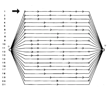
to at most one per management alternative was made in order to reduce the number of alternatives (variables) required by this f6rmulation. Figure 2.2 is digraph representing

the structural constraints (2.10) when more than one crop-type is present.

Any model I management unit can be considered to be a network as in Figure 2.2. Generally, the harvest patterns will differ depending on the establishment period, the

minimum and maximum ages of clearfelling for the initial and subsequent crop-types. Because paths in the network have to be constructed for each of the subsequent crop-types, the number of variables required to formulate a model I

approach quickly increases.

Management alternative

2 3

Period Number

4 5 6

2 3

4

5 6 7 8

9

10

11

1 2

13 14 15

16

1 7

18

19 20 21

Figure 2.2 Diagraph showing model I management alternatives

The harvest pattern for the alternatives 1 through 21 in Figure 2.1 is indicated. vertices (when present) along each path from the vertex labelled a to the vertex labelled w denote a harvest. Paths between a and the first harvest vertex (when present) correspond to the growth of the initial crop-type, subsequently each path represents growth and possible harvest of the

an example of a digraph corresponding to such a constraint set.

where

Model II multiple crop-types structural constraints

2

=

I

j k

(2.11)

T+1

I

tki

=

l

k s==t+1

s,~,s-(2.12)

T+1

a, _~j +

l

-

I

I

k k s::::l

(2.13)

(2.14)

i

=

=

ik

0.' .

I~

. I

are the units of area clear felled in period t from crop-type i and age class j;

are the units of area clear felled in period t from crop-type i and immediately replanted into crop-crop-type k;

are the units of area transferred from crop-type i and age class j to crop-type k. These transfers are made at the commencement of the initial planning period;

J'S the ,,...\\,0..\ (veG.. o."o..,lt\.~lt

ot

is the number of crop-types either initial or reafforestedj J is the oldest initial age class; and

T is the number of planning periods.

Equation (2.11) implies that, for crop-type i in any period t, the subscript j runs up to the oldest initial

age class J. In general, for period t, the subscript j must range over the age classes that may be present in period t and may be harvested. Equation (2.11), in terms of the oldest initial age class, should then be specified as

J+t-1

I

j ::::1

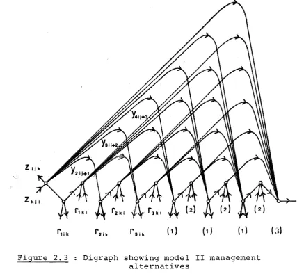
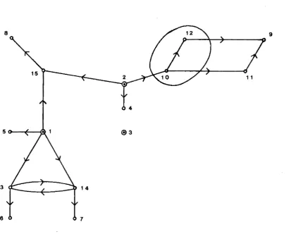
Figure 2.3 Digraph showing model II management alternatives

A single crop-type it initial age class j, is scheduled over six periods using equations (2.12) through (2.15). The crop-type is of harvest age in the initial planning period. Subsequent rotations of the same crop-type have a minimum rotation length, of two periods (c.f., Figure 2.1).

The digraph in Figure 2.3 represents exactly the same management possibilities as found in Figure 2.1. Equations

(2.15), (2.12), and (2.13) represent the areas entering and leaving vertices of the types labelled (1), (2), and (3) respectively in Figure 2.3. The dangling arcs, that is, the arcs without vertices attached, are included for complete-ness only, (rtik's, Zijk's) in that they would all have value zero in this example. Arcs of the form r

t ~~ ,. are not dangling

By inspection of Figures 2.2 and 2.3 i t is evident that they do not have the same structure [they are not

isomorphic to each other, (see Robinson and Foulds, 1980)), in that each vertex in Figure 2.2, excepting the source and the sink, has one arc entering and one arc leaving, whereas this does not hold in Figure 2.3. Clearly, digraphs such as these can be used to show the difference in representing model I and model II management units.

The variables actually specified in the set of structural constraints depend on the age classes initially present for

each crop-type, the minimum and maximum age of c1earfe11ing, and area transfers. This will always be less than or equal to the number of variables specified by equations (2.12) through (2.15). Thus, these equations specify a superset of the variables actually used. The structural constraints are presumably specified in this way in order to reduce the subscripting complexity that would arise should an attempt be made to subscript the variables actually used. Garcia

(op. cit.) uses a computer program that specifies as part of its input the necessary subscripting information to generate the required problem and, in this way, overcomes the difficulty of working with a perhaps difficult set of subscripts.

The model I and model II formulations differ in

terms of the number of variables required to represent them. As the size of the problem becomes larger, the model II

formulation becomes more efficient in terms of the number of variables used. The following procedures can be used to enumerate the variables required by each model.

The number of variables required by a model I

number of paths in the digraph representing the structural constraints. On the other hand, for a model II formulation, i t is equal to the number of arcs in the digraph representing equations (2.12) through (2.15). The problem of counting these arcs can be simplified. If these equations were to consider only a single crop-type then all r 'k's and z .. 's

t 1 1 Jk

could be dropped. Thus, in Figure 4, the vertices labelled (1) and (2) would become the same (co-incident) and the number of arcs in the remaining subdigraph could be computed using the formulae of Johnson and Scheurman (1977). Clearly, the number of variables needed for a model II with mUltiple crop-types could be determined by using the formulae to

calculate the number of Yt' ,s for each crop-type, aggregating

1J

over crop-types, and including the number of ways of trans-ferring area between crop-types, that is, the number of rtik's and z, 'k' S •

1J

2.2.5 Multiple Crop-type Regulatory Constraints

As indicated in SUbsection 2.3.3,linearcombinations of the structural variables within a model I and II formulation that can be used for regulatory purposes are easy to construct. To facilitate the specification of these for model II, Garcia

(1984) specifies the residual area after the harvest of crop-type i age class j in period t to be given by equation

(2.16)

where

T+l X

tij :=

L

5=t+l

is the residual area after harvest of crop-type i age class j in period t.

The linear combinations for total harvest volumes for model I and model

tI

(2.18)

where

I J. 1 K .. 1J L. 'k 1J

h =

I

L L L

_v,

i=l j =1 k=l 9.=1 1 J n

(2.17)

I J+n-l T+l

h =

L I

I

i=l j=l t=n t1Jn

(2.18)6

V, 'k9. is the volume per unit area produced in period n 1 J n by management alternative 9., whose initial crop-type

is i, initial age class j, and whose regeneration crop-type is k

V , ,

t1Jn is the volume per unit area produced in period n by crop-type i that is clearfelled in period t

when in age class j.

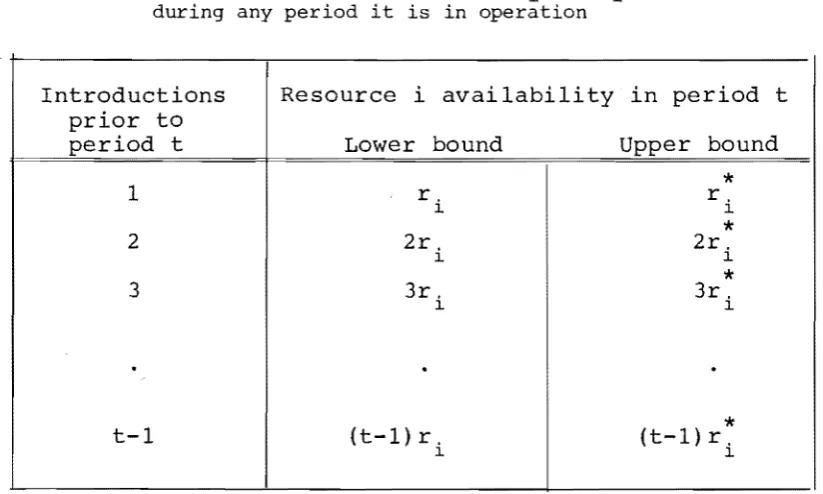
The implementation of regulatory constraints usually requires the concise definition of the resource sets that are being regulated. Typically a resource can be any commodity that characterises forest growth and is readily quantifiable .' _, This criterion of qu~ntifiability is partic-ularly important in that the inclusion of imprecise data

items in mathematical programs representing forest management problems can have deleterious effects (Rose, 1984). This suggests that suitable resources might be those commodities that can be measured in terms of area or volume, these being the most precise measures available for characterising forest growth. Consider, for example, a log class set that is

rigidly defined by log grading rules, then the volumes either standing or harvested for members of the log class set could

6 _{Not all terms in the summation are necessarily defined. The}

be used as a resource set. Similarly, the areas of crop-types either standing or harvested in any period can be used as a resource set.

The choice of what constitutes a suitable resource set to describe output from a forest is, in New Zealand, a matter of contention at the time of writing. However, within models representing forest management problems or

forest utilisation management problems, the definition of such resources sets is crucial. It governs the description of material to be received by processing centres that utilise

forest resources and, for FUMPs, the definition of processes within those centres. A discussion of the attributes suitable

for the classification of resources output from a forest, in the case when resources are considered to be logs, is given in section 3.1 of Chapter 3. These attributes must be sufficiently detailed so as the various log input require-ments of different ultilisation processing centres can be

specified in terms of the attributes.

2.3 BOUNDING AND SMOOTHING REGULATORY CONSTRAINTS

Provided that the resources to be regulated are

adequately defined and can be expressed as linear combinations of the structural variables within a model I or model II

formulation, then regulatory constraints can be imposed. Generally, such constraints are considered to be either smoothing or bounding. This section considers the develop-ment of a class of constraint that is both smoothing and

Smoothing constraint set

(1+y, ,)r

i ,

l.J J

- r .~ 0

i j +1 ' Vi, j (2.19)

v· ,

,th

i is the index of the 1. resource

j=1, ... N-1, is the index from the time set where

y " , 0 .. are scalars such that (l+Y .. ), (1+0, ,) >0, and

1J l.J l.J l.J

r.. is the measure of resource i at time j, and r. , ~ 0

l.J 1J

Consider the following in relation to (2.19) above 7 Case one

r

k

=

k

=

J for 1 ~ j ~ k -1 since r. J ~ 0, (1+y .) J ~ O.

Case two r

k > 0 for k £ {I, . . . , N-1 } if r

k > 0 then by (2.19) r, > 0

J for k+ 1 ~ j ~ N.

Case one suggests that, should the resource measure at any period, except the first, become zero, then the resource at all previous periods is constrained to be zero. Case

two suggests that, should the resource measure at any period, except the last, become positive, then the resource measure at all succeeding periods will become positive.

Bounding constraints can be formulated using the system (2.19), which implicitly satisfy the systems (2.21) and (2.25). The proofs are given in the following lemmas.

7

Lemma 2.1

Given the constraint system (2.19), show that r. 1 ,) ( 1 +y

t>

J+ ]

for j=l, ... ,N-l. Proo : by induction

P(l) is obviously true from the system (2.19), assume P(k) true, k = 1, . . . ,N-2. An induction proof requires that P(k+1) holds. P(k) true implies (2.22)

multiply both sides of (2.22) by (1+Yk+1)' then (1+Yk+1)r

k+1 ,) (1+Y 1) (1+y2) ••• (1+y k+1 )r1

Consider the constraint system with j=k+1, then

Jointly, (2.23) and (2.24) imply P (k+1) . Lemma 2.2

Given the constraint system (2.19), show that rN

r . ~

---N-]

(1 +y N _ j) ••• (1 +Y N _ 2) (1 +y N -1 )

j

=

(2.21)

(2.22)

(2.23)

(2.24) o

(2.25)

To establish p(l) set J = N-1 in the constraint system, then

r ~

N-1 _l+y N-1

and P(l) is true, assume P(k) true for k=l, . . . n-2, P(k) true implies

r ~

Multiply both sides of (2.26) by

~~-=1

(l+YN_ (k+1)) , then

r

N-k

(l-+y_{N _ (k+l»)} (2.27)

Consider the system (2.19) with j

=

r

N-k

(2.28)

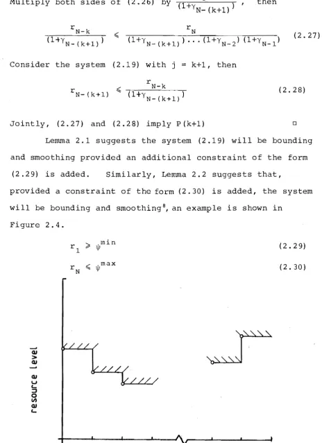
Jointly, (2.27) and (2.28) imply p(k+1) o Lemma 2.1 suggests the system (2.19) will be bounding and smoothing provided an additional constraint of the form

(2 . 2 9) is adde d . Similarly, Lemma 2.2 suggests that,

provided a constraint of the form (2.30) is added, the system will be bounding and smoothingS

, an example is shown in Figure 2.4.

-

>

OJ

-

u

3

o

V)

QI

c...

Figure 2.4

(2.29) (2. 30)

2 3 N-1 N

time

A Resource Lower Bound Envelope

The envelope is formed using (2.19) and (2.29), feasible resource amounts at each model period lie above the shaded horizontal lines.

a

Similarly, the system (2.20) can be used to develop constraints that are both bounding and smoothing, however, the behaviour of this system is initially examined in cases three and four below.

C e three r

k = 0 for k

=

k == 0 then by (2.20) and induction r. == 0 for k+1 ~ j ~ N

.

J

Case four r

k > 0 for k == 2 , •.• , N if r

k > 0 then by (2.20) and induction

r. > 0 for 1 ~ j ~ k-1.

J

Case three suggests that, should the resource measure at any period, except the last, become zero, then the resource measure at all succeeding periods will be zero. While Case

four suggests, that should the resource measure at any period, except the first, became positive, then the resource measure in all previous periods is constrained to be positive.

The following Lemmas arise in conjunction with (2.20). Lemma 2.3

Given the constraint system (2.20), then

r

j +1 ~ (1+01) (1+02) " , (1+oj )r1 vj j == 1, .•• ,N-1.

Proof (omitted)

(2.31)

The proof is by induction and closely parallels the proof of Lemma 2.1

Lemma 2.4

Given the constraint system (2.20), then rN

r . ~

N - J (1 +0 N _ j) ••• (1 +0 N _ 2) (1 +0 N _ 1)

j :: 1, ... , N-1 •

o

Proof (omitted)

The proof is by induction and closely par ls the

proof of Lemma 2.2 o

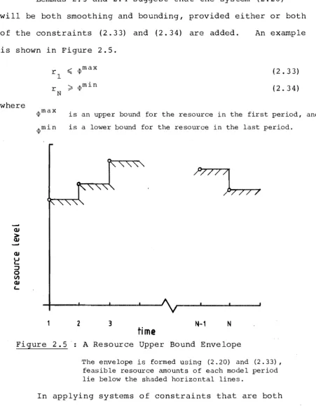
Lemmas 2.3 and 2.4 suggest that the system (2.20) will be both smoothing and bounding, provided either or both of the constraints (2.33) and (2.34) are added. An example is shown in Figure 2.5.

where

-

-

t!

o

II)

OJ

c...

r

1

<

max r ~ <pmin

N

(2.33) (2.34)

<pmax is an upper bound for the resource in the first period, and <pmin is a lower bound for the resource in the last period.

/'777J

"'7""""7""7""-/7

2 3

N-1

time

Figure 2.5 A Resource Upper Bound Envelope

The envelope is formed using (2.20) and (2.33), feasible resource amounts of each model period lie below the shaded horizontal lines.

In applying systems of constraints that are both bounding and smoothing, a reduction of constraints

application requires that careful consideration be given to how the bounding and smoothing system operates. This may be done by considering cases one through four above. The choice of which system to apply might take into account such aspects as the accuracy of the bound. For example, it may be easier to determine a bound for the initial period because the estimation period is shorter and the precision of estimate is likely to be higher than for the final period. Consider-ation could also be given to applying such constraints over a subset of time periods, creating partial envelopes of smoothing and bounding constraints. Finally, i t may be better to only smooth some resources rather than smooth and bound them. For example, depending on how the constraints are formulated the addition of bounding constraints may unnecess ly impose a pattern of resource consumption or production, in all model periods.

2.4 SOLUTION TECHNIQUES FOR FOREST MANAGEMENT PROBLEMS

Historically, the development of mathematical programs to represent forest management problems have evolved from a class of programs that allowed only a narrow range of

management criteria to be specified to one that permits both generalised structural and regulatory constraints and is

typified by the models of Hoganson and Rose (1984) and Garcia (1984) which are respectively model I and model II in terms of their structural constraints.

Similarly, the methods used to solve FMPs have

Berck and Bible, 1984; Garcia, 1984). A method that

considers both structural aspects and the possible imprecision and inaccuracy of data items has also been proposed (Hoganson and Rose, 1984).

This section discusses solution techniques, their evolution in relation to the class of FMP being solved, and the method employed. Subsection 2.4.1 discusses applications of the simplex method; subsection 2.4.2 discusses a model I decomposition technique; subsection 2.4.3 discusses a model II decomposition technique; and subsection 2.4.4 discusses a solution method based on the estimationof certain key dual variables.

2.4.1 Standard Simplex Methods

Conceptually, all linear programming problems can be solved by application of the simplex procedure, but practical limits exist as to the size of problem that can be solved using such central algorithms as the revised

simplex method. At the time of writing, the magnitudes of 20,000 variables and 15,000 constraints (approximately) define the range of the revised simplex procedure9 •

Currently, major linear programming generators and report writers are used for generating and reporting on FMPs that are to be solved using the revised simplex procedure. Amongst these are the systems, MAX-MILLION (Clutter, 1968), TIMBER RAM (Navon, 1971) and FORPLAN (Johnson et

at.

Although the development work for such systems was chiefly undertaken in the united States, work has also been under-taken in Australia (Paine, 1966, cited in Clutter et

at.,

1983) and New Zealand (Shirley, 1978; Garcia, 1984). 9

Compact inverse techniques and sparse matrix techniques are sometimes used in conjunction with the revised simplex method to increase its

Johnson and Scheurman (1977) consider solution

techniques to various simple FMPs, that would otherwise be solved by simplex methods, by specification of the Kuhn Tucker conditions (Walsh, 1975). Where the objective function is linear or quadratic and the constraint set is linear, these conditions are both sufficient and necessary for global optimality. In the situations outlined by

Johnson and Scheurman (op. cit.), solutions to the mathematical program representing the FMP can in some circumstances be

obtained by direct application of the Kuhn Tucker conditions. In others, the conditions serve as the basis for algorithms to solve the FMP without having to perform the simplex

procedure.

The model of Ware and Clutter (1971) is arguably the most famous model I formulation to be solved using a standard

simplex procedure. Appendix 2.4.1.

The form of this model is indicated in

2.4.2 Decomposition Methods Model I

All Forest Management Problems, when formulated as linear programs that have structural constraints that can be classified as model I or model II, have constraint

matrices that are highly structured. These structural matrices arise because problem formulation requires the repeated

where

m n

maximise z :::

~

I

i=l j=l 1.j 1.J s.t.

u.

+

J J J J

m

I

+

₌

n

I

₌

r. are units of area in management unit i

1.

(2.35)

(2.36)

(2.37)

(2.38)

bmin b~ax

j , J are minimum and maximum units of area that may be cut in year j

C . .

1.) in the yield from management unit i if cut in year j

x ..

1.) is the proportion of management unit i to be cut in year j, and

u., v.

J J are slack and surplus variables for units of area to be cut _{in year j.}

The decomposition procedure results in a subproblem

that is easy to solve by inspection. This arises by placing all constraints of the form (2.38) in the subproblem. Tcheng's method has only one convexity row for the subproblem, it

solves linear programs at the level of the subproblem by inspection and performs pivot operations at the level of the master to introduce the new column to the basis. These pivot operations ensure primal feasibility. Thus the slack variable constraints are satisfied (Lasdon, 1970).

Note that if Tcheng's methods were adopted to solve linear programs at the level of the subproblem and the master, by decomposing with m convexity constraints in the subproblem

(the number of management units) and using the candidate solutions from each subproblem at the master level, then the master program resulting would have the same number of

constraints as does the original problem, and so no reduction

2.4.3 Decomposition Methods Model II

Recently, decomposition methods have been proposed for FMPs that possess model II structural constraints

(Berck and Bible, 1984; Garcia, 1984). Of these proposed methods, that of Garcia's is more flexible because the model allows area transfers and multiple crop-types to be

specified. Garcia's decomposition technique, therefore, is outlined in this section.

As with a model I decomposition, i t is the structural constraints that form the constraint set for a model II

subproblem. These are equations (2.12) through (2.15).

These constraints were illustrated in Figure 2.3 for a single crop-type i and single age class j scheduled over six planning periods. It is very easy to envisage Figure 2.3 when more than one crop-type i is present. Furthermore, each crop-type may have a number of initial age classes. The resulting

digraph may be converted into an acyclic network by appending a dummy source and dummy sink and breaking any cycles that may occur at points labelled (3) in Figure 2.3. Flows in this network will be area flows; moreover flows along each arc are uncapacitated, which means that the optimal flow in such a network will be the minimal cost flow __

Thus, solution of the subproblem in Garcia's formulation requires the identification of minimal cost paths in an

acyclic network. This constitutes a well known network problem. A solution to such a problem can be obtained

by constructing a solution to the dual of the network problem, and then identifying the solution to the primal problem from the optimal dual solution; the method is outlined in Wagner