A study in beamforming and DAMAS deconvolution

Internship report

A study in beamforming and

DAMAS deconvolution

A.J. Bosscha

Abstract

Auroacoustic wind tunnel experiments are nowadays performed with phased array measurements. A large array of microphones captures data and to-gether this data can be processed to gain insight the behaviour of the acoustic sources of the test subject. The regular way to prosses this data is by con-ventional beamforming. Comparing the cross specra of the microphones with a reference monopole source tells a lot of the acoustic sources the test object produces.

Using this beamforming data in the DAMAS deconvolution method gives even better insight in acoustic behaviour. DAMAS deconvolution is an iterative method which can predict the locations of acoustic sources in a much better way than conventional beamforming.

There are two possible ways to extract amplitude of sources out of con-ventional beamforming or DAMAS plots; using an integration method of using the peak levels of the plot. When investigating line sources, the peak level method gives an off result. The height of this off result seems to differ for various coherent lengths of the line source.

A calibration function is made, which compensates for this off result, so the peak level method can also be used to find the strength of line sources. This calibration function is made for several coherent lengths.

Also a method is discussed to extract coherence length out of experimen-tal data. However, this can only be done on a visual manner, therefore the possibility of making an error is high. Due to this error in coherence length es-timation, the wrong calibration value can be picked, which results in an error up to 2dB.

N

OMENCLATURE

Ann0 Influence of beamforming characteristics between grid pointsnandn0

B Beamwidth

Gmm0 Cross spectrum between microphonemandm0

I Sound intensity M Mach number

N Total number of grid points ·0 _{Fluctuation of variable·}

·H _{Hermitian operator}

i Imaginairy unit;√−1

ˆ

A DAMAS matrix withAnn0 components

ω Angular frequency

ρ Density

ˆ

G Cross Spectral Matrix (CSM) ˆ

d Steering vector ˆ

e Steering vector u Velocity

c Speed of sound f Frequency [Hz]

m Microphone identy number in the array m0 Same asm, but indepandant varied m0 Total number of microphones in the array n Grid point identy number in the array n0 Same asn, but indepandant varied

p Pressure

C

ONTENTS

1 Introduction 3

2 Sound propagation 5

2.1 Wave equation . . . 5

2.2 Harmonic point source . . . 7

3 Coherence 8 3.1 Interference . . . 8

3.2 Wave trains . . . 8

4 Beamforming 11 4.1 Fundamentals of conventional beamforming . . . 11

4.2 Cross Spectral Matrix data . . . 13

4.3 Accounting for uniform flow . . . 13

4.4 Sidelobes . . . 14

4.5 Noise and reflections. . . 14

5 DAMAS deconvolution 17 5.1 Defenition inverse problem . . . 17

5.2 Solution inverse problem. . . 18

5.3 Application parameters . . . 19

5.4 DAMAS results . . . 19

6 Experimental set-up 23 6.1 Coherent line source . . . 23

6.2 Synthetic CSM . . . 23

6.3 Wind tunnel dimensions . . . 23

6.4 Array. . . 24

6.5 Results . . . 24

7 Array Calibration Function 27 8 Determination of coherence levels 29 8.1 Incoherent monopoles . . . 29

8.2 Line source . . . 29

1. Introduction

The last 100 years a lot has changed in our ways of transportation. In the past men had to use roads, railways or waterways to transport passengers and goods, but since the invention of the aircraft a whole new era begun.

Nowadays aircraft are widely used for transportation. The whole world is easily accesible for work or vacations. This great increase in aircraft usage however, also has some downsides. Commercial airfields, usually located in densed areas, are coping with noise problems. An aircraft at takeoff or landing produces quite an amount of noise, and with lots of departing and arricing flights per airfield, the people (and animals) living nearby are having quite some noise pollution. This is why airfields have to comply with strict noise regulations.

If an aircraft produces less noise at takeoff or landing, the effective capacity of the airfield increases, which means more profit for the airfield and econom-ical growth for the whole region. At the takeoff of an airplane, the turbines are the dominant factor in the production of sound. At the landing however, the sound produced by the wings (flap and slat) and landing gear are the domi-nating sources.

Aircraft manufacturer Embraer and the aeronautica group of the University of S ˜ao paulo together have started a collaboration project - the Silent Aircraft Project. The goal of this project is to investigate (and reduce) the sound cre-ated by flap, slat and landing gear of Embraer aircrafts. To gain insight in the behaviour of flap, slat, and landing gear induced sound, both numerical simulations and wind tunnel experiments are performed.

Nowadays acoustic wind tunnel experiments are performed with a micro-phone array. The data from a great amount of micromicro-phones is combined to find the acoustic behaviour of the test subject. The difference in phase and amplitude of the different microphone signals is used to find location and am-plitude of the sound sources, therefore this technique is called phased array testing.

The data proccessing thechnique used to locate sound sources and ampli-tudes is called Conventional Beamforming. This process can acquire, given a certain grid, the locations where there is a high probibility of finding an acous-tic source. However, this technique has some downsides; the peak levels of line sources are presented wrong for example [1].

To gain even better insight in acoustic behaviour a method called DAMAS deconvolution is used [4]. This method uses the conventional beamfoming spatial plots for its expectation of source locations. The spatial detail of this method is much larger than the results of the conventional beamforming plots. However, also DAMAS deconvolution copes with the problem the peak levels of line sources are wrong.

of the line source also seems to contribute. Therefore the calibration function is made for several coherent lengths of line sources.

2. Sound propagation

Sound can be seen as a weak pressure disturbation which travels through a fluid. The perturbation moves through the fluid as a wave and causes small variations in the velocity and density of the fluid.

Altough the acoustic pressure fluctuations are small compared to the mean (atmoshperic) pressure, the range in amplitudes is very large. This makes it convenient to express pressure amplitudepon the logarithmic scale:

SP L(dB) = 20 logprms

pref

(2.1) where SPL is the sound pressure level in decibels, prms the

root-mean-squared value of the pressure andpref the reference pressure of2·105P a.

Since disturbances are small, the variables have to satisfy the linearized equations of fluid motion. For sound propagation inertial forces are usually much larger than viscous forses. Effects of viscosity can therefore be ne-glected when examining acoustic wave propagation.

2.1

Wave equation

Consider a fluid with velocityut, densityρtand pressurept. From the

conser-vation of mass it follows that ∂ρt

∂t +∇ ·(ρtut) = 0 (2.2)

Conservation of momentum gives ∂(ρtut)

∂t +∇ ·(ρtutut) +∇Pt=f (2.3) where ∇ is the nabla operator (∂/∂x, ∂/∂y, ∂/∂z), f the density of the external force field acting on the fluid and Pt = ptI−τ is the fluid stress

tensor. By neglecting viscosity and using the conversation of mass (2.2) the conservation of momentum (2.3) can be written as the Euler equations [5].

ρt

_∂u

t

∂t +ut· ∇ut

+∇pt=f (2.4)

Considering small perturbations of velocity, pressure and density, equation (2.2) and equation (2.4) can be linearized. We writeut =u0+u,pt=p0+p

andρt=ρ0+ρ, where the subscript ’0’ indicates the uniform mean value and

mean velocityu0=U andf = 0, the linearized equations for conservation of

mass and momentum can be rewritten as

∂ρ

∂t +U· ∇ρ+ρ0∇ ·u= 0 (2.5a) ρ0

_∂u

∂t +U· ∇u

+∇p= 0 (2.5b)

If the uniform quantitiesU,p0andρ0are known, equations (2.5) only pro-vide four equations for the five unknownsu,pandρ. The additional informa-tion can be found in the constituinforma-tional equainforma-tions. We assume the fluid to be in a state of thermodynamic equilibrium. This means we can write the pressure ptas a function of the densityρtand entropyst.

dpt=

_∂p

t

∂ρt

s

dρt+

_∂p

t

∂st

ρ

dst (2.6)

Momentum and heat transfer are controlled by the same molecular colli-sional prosess. If we neglegt viscosity, we should also neglect heat transfer, and therefore the flow is isentropic. This means the entropy of a fluid particle remains constant and thereforedst = 0. By defining the speed as sound as

c2_{= (∂p}

t/∂ρt)s, equation (2.6) becomes

p=c2₀ρ (2.7)

wherec0=c(p0, ρ0)is used to approximate the speed of soundc.

Using equation (2.7) we can write ρin terms ofp. Using this in equation (2.5a) and substracting the divergence of equation (2.5b), velocityuis elimi-nated and the convective wave equation is obtained.

1

c2 0

∂

∂t+U· ∇ 2

p− ∇2_{p= 0 (2.8)}

For many application this equation can be simplified by assuming zero mean flow (U = 0). This equation is called the wave equation of d’Alembert.

1

c2 0

∂2_p ∂t2 − ∇

2_{p= 0}

(2.9) Transforming d’Alemberts wave equation to spherical coordinates and as-suming the pressure field is axi-symetric gives the following equation. The productrpsatisfies the one-dimensional wave equation.

1

c2 0

∂2_rp ∂t2 −

∂2_rp

∂r2 = 0 (2.10)

Solving this equation gives the expression for an outward propagating har-monic spherical wave.

p(r, t) =Ae

iω(t−r/c0)

r (2.11)

2.2

Harmonic point source

Up now we have considered propagating waves whose behaviour is governed by the homogeneous wave equation (2.9). This equation however, only de-scribes the propagation of sound generated at boundaries, incoming sound fields from infinity or sound due initial perturbations. A sound sourceq(x, t)is defined, which produces sound at a certain locationx.

1

c2 0

∂2p ∂t2 − ∇

2_{p=q (2.12)}

The source region, whereqis non-zero, is separated from the sound field, whereq is zero and the propagation of sound waves is governed by the ho-mogeneous wave equation. Where qis non-zero the sound field is uniquely determined by the given initial and boundary conditions.

q(x, t) =δx−xsσs(t) (2.13)

3. Coherence

In this chapter the meaning of coherence is explained, but to do so first the subject interference will be examined.

3.1

Interference

A pressure field often contains sound waves from different sources. Assume the spatial parts of two pressure waves are described by:

p1=A1e−iφ1 _(3.1a)

p2=A2e−iφ2 _(3.1b)

whereφ1 andφ2 are functions of position and represent the phase shift of the waves. The superposition principle may be applied and the resulting pressure field becomes merely the sum of the two individual fields.

p=p1+p2 (3.2)

The observed quantity is, however, the sound intensity.

I=|p|2

=|p1+p2|2

=A2₁+A2₂+ 2A1A2cos(φ1−φ2)

=I1+I2+ 2 p

I1I2cos(∆φ)

(3.3)

where∆φ is the difference in phase between the two waves. As it can be seen, the sound intensity does not become merely the sum of the two intensities. The term2√I1I2cos(∆φ)is called the interference term [2].

Detection of sound by a microphone is an averaging process in time. In developping equation (3.3) no averaging over time is done, because it is as-sumed the phase difference ∆φ is constant in time. This also means it is assumedp1andp2have the same frequency.

3.2

Wave trains

p1

Lc Lc

p2

(a) Partial wave 1 is the same as partial wave 2

p1

Lc Lc

p2

(b) Partial wave 2 is completely different as partial wave 2

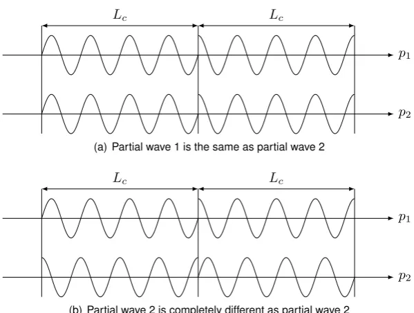
Figure 3.1: Wavetrains

abrupt, arbitrary phase change takes place. In figure3.1(a)both wave trains have traveled equal distance. Between the two waves, the phase difference is equal in time. The intensity of these waves is given by equation (3.3).

Since the phase difference between the two partial waves is absent, the sound intensity of the field becomes I1+I2 + 2√I1I2. When both partial waves have the same sound intensityI0, the sound intensity becomes4I0. In this case the partial waves are called fully coherent.

In figure 3.1(b), the second partial wave has traveled exactly one wave train length (Lc) further then the first partial wave. The sound intensity is still

given by equation3.3. The phase difference now fluctuates randomly as the wave trains pass by. This means the partcos ∆φseen in the interference term fluctuates between−1 and+1. When averaged over many wave trains, the interference term becomes zero, and the observed intensity will be I1+I2. If both partial waves have the same intensity I0, the amplitude of the field becomes2I0. This case is called the incoherent case. Cases between fully coherent and incoherent are called partial coherent. However, in this report only the incoherent and fully coherent cases will be examined.

Figure3.2represents a line source. When looking at some points located at the line source at positionxi, we can tell something about the coherence

Line source

x1 x2 x3

High coherence

Low coherence

4. Beamforming

In aeroacoustic testing, a model is exposed to a flow. This flow causes the model to produce a complex array of sounds. Often several parts of the model have interesting noise production worth examining. These different sources create sounds in a wide frequency spectrum and different tone.

A technique often used to get an insight in the location and strength of these different sources is phased array testing. In phased array testing, sev-eral microphones can be used together to extract source location and strength information from noisy, non-acoustic wind tunnels.

The basic phased array processing step is called beamforming. Beam-forming has a long history in radio atronomy, but can also be applied to acous-tic problems. The beamforming process uses a mathemaacous-tical model for the acoustic propagation from each grid point to each microphone. Cross spectral data between different microphones is used to gain insight in acoustic source distribution.

4.1

Fundamentals of conventional beamforming

The general idea of beamforming signal processing is to compare the data measured by the array of microphones with a reference pressure. As ref-erence pressure an harmonic monopole source is taken. By minimizing the squared norm of the difference between these two quantaties, a good esti-mate of the source location and strength is given.

In equation 4.1 pˆrepresents the spatial pressure component of the ref-erence pressure, a singal emitted by a monopole source at location rs at a

specific frequencyf. The variableasrepresents the complex amplitude of this

monopole source, which may vary for different frequencies and positions.

ˆ

p(as,rs,r) =

ase−ik|r−rs|

4π|r−rs|

(4.1) Equation4.1can also be written aseaˆ s, where each term of column vector

ˆ

e represents the reference signal for a different microphone. eˆis also called the steering vector.

All thek-th Fourier transform coefficients of a real signal recorded by the microphone array are stored in column vector P. The length of the vector equals the number of microphones. By defining a cost function J (4.2), an estimate ofascan be made by minimizing this function.

J(ω,as,rs) =||ˆeas−P||2 (4.2)

Usingu = eaˆ s−P and the identity shown below (4.3), the derivative of

the cost function (4.2) can be expressed. d

du(u

H_{u) = 2u}H_I

In this equationIrepresents the identity matrix. dJ das = dJ du du das

= 2(eaˆ s−P)Heˆ (4.4)

The cost function is minimal if derivative of it (4.4) is zero. Using the identity AHB=ABHthis can be rewritten to:

ˆ

eHˆeas=eˆHP (4.5)

Which leads to the least square solution ofas.

˜

as= (eˆHeˆ)−1ˆeHP =

ˆ eHP

||ˆe||2 (4.6)

Below the cost functionJ is expanded in terms ofas.

||ˆeas−P||2= (eaˆ s−P)(ˆeas−P)H

= (asHˆeH−PH)(ˆeas−P)

=asHeˆHeaˆ s−2asHˆeHP +PHP

(4.7)

Using the least square solution ofasgives:

J(ω,rs) =PHP −

(eˆHP)H_(eˆH

P)

ˆ

eˆeH (4.8)

The termPHP represents the sum of all auto spectra of the array. Be-cause it is derived directly from the external sound field, it does not depend on the parameters used to model the acoustic field, and can be seen as a constant in this formulation.

I(ω,rs) =

(ˆeHP)H_(eˆH

P)

ˆ eHeˆ

= eˆ

H

||ˆe||P P

H eˆ

||ˆe||

= eˆ

H

||ˆe||Gˆ ˆ e ||e||ˆ

(4.9)

The matrixGˆ is called the cross spectral matrix (CSM), and contains the time averaged data of the microphones. When there are m0 microphones used in the array,Gˆwill have anm0×m0size.

ˆ G=      

G11 G12 · · · G1m0

..

. G22 ...

..

. . .. ...

Gm01 · · · Gm0m0

      (4.10)

xe

x xs

θs θe x

ct r

wavefront

wind

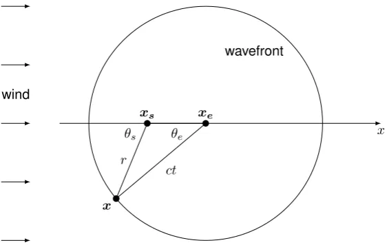
Figure 4.1: Wavefront in uniform flow

4.2

Cross Spectral Matrix data

When doing wind tunnel experiments, large amounts of data are obtained. All microphones gather data during the time of the experimentTtot. To gain

insight in the acoustic behaviour of the flow, the data is time averaged. As stated in section4.1, first the Fourier transform of each microphone is taken. This gives different data sets per frequencyf, which are∆f apart from each other. Afterwards, each data sample is divided into several blocks of timeT.

Gmm0(f) = 2

KwsT K

X

k=1

[P_mkT (f, T)Pm0_k(f, T)] (4.11)

The cross spectrum is averaged overKblock averages. The termwsis a data

window weighting constant - often Hamming windowing is used.

4.3

Accounting for uniform flow

In the determination of steering vector e, it is assumed the sound wavesˆ pass through a non-moving medium. However, in windtunnel experiments the medium (air) moves at a certain speedU. To take acount for this, a correction to steering vector is made.

Assume the time it takes for a sound wave to travel from the source to the microphone, in the non-moving medium case is ∆t. When the medium moves uniformly at a certain speedU, the sound waves travel a distanceU∆t downstream.

Figure 4.1gives a scematic overview of the situation. xs is the location

of the source. Because the sound waves move downstream, the observerx thinks the source is located atxe.

Rewriting this in terms of mach numberM, gives a new corrected steering vector.

ˆ e= R

rc

Where R and rc are corrected with the Doppler amplification factor 1−

M2. rc is the corrected distance from the observing point to the center of the

coordinate system.

rc=

p

x2_{+ (1−M}2_)(y2_+z2_{) (4.13)} Ris the corrected distance from observing point the the source location.

R=p(x−xs)2+ (1−M2)((y−ys)2+ (z−zs)2) (4.14)

T =−M(x−xs) +R

(1−M2_)c (4.15)

Using this steering vectoreˆthe system is adapted for uniform flow of mach numberM.

4.4

Sidelobes

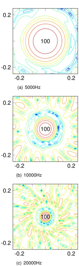
The output of the beamform algorithm relies ofcourse on the sound sources. However, when sound source is taken constant, differences in the spatial beamforming map can be seen for different frequencies and array designs. At higher frequencies, small peaks can be seen on locations that are not at a sound source. These small peaks are called sidelobes. The main lobe is the is the peak resulting from the sound source.

In figure4.2the sidelobe effect can be seen for different frequencies. The figures clearly show the sidelobe effect increases for increasing frequencies. At 5000Hz almost no sidelobes are seen, but at 20000Hz the sidelobes are almost at the same strength as the main lobe.

The sidelobe effect can be resolved my putting a treshold on the beam-forming map. Every value which is a set value lower that the highest peak level, gets removed. This treshold is often called dynamic range. It should be noticed that by using a treshold, it is also possible to remove main lobes with less strenght than the strongest main lobe.

4.5

Noise and reflections

When performing acoustic experiments, it is impossible to have the perfect conditions. All kind of imperfections make it difficult to compare experimental results with the theory, which asumes a perfect anechoic wind tunnel facility and no noise.

No windtunnel is completely anechoic, so the microphone array will notice the reflections of the sound waves against the wind tunnel walls. However, us-ing good isolation against the walls these reflections can be greatly reduced. Reflections of sources are fully coherent with their origional source. In chap-ter8this property is used to to find reflections or sidelobes.

Intermittend sounds, like people talking outside the windtunnel, are random and can be took out by time averaging.

-0.2 0.2 -0.2

0.2

100

(a) 5000Hz

-0.2 0.2

-0.2 0.2

100

(b) 10000Hz

-0.2 0.2

-0.2 0.2

100

(c) 20000Hz

noise is generally incoherent from one microphone to the other, it will only appear in the auto spectra of the CSM. Removing the auto powers (Diagonal Removal) of the CSM, can remove this floor of noise from the beamforming spatial maps.

5. DAMAS deconvolution

The processing of array data with the conventional beamforming technique (chapter4) is burdened with considerable uncertainty. The Deconvolution Ap-proach for the Mapping of Acoustic Sources (DAMAS) removes beamform characteristics from the output presentation. Using the DAMAS deconvolu-tion method, misinterpretadeconvolu-tions are reduced when quantifying posideconvolu-tion and strength of acoustic sources.

First an inversed beamforming problem is defined, which results in a set of linear independant equations. Afterwards these equations are solved using a special iterative algorithm.

5.1

Defenition inverse problem

The pressure transformPmof microphonemis related to a modeled monopole

source located at positionn.

Pm:n=Qne−m1:n (5.1)

The terme−m1:n is simply the inversed steering vector. The product of

pres-sure transforms now becomes

P_mT_:nPm0_:n= (Q_ne−_m1_:n)T(Q_ne−1

m0_:n) =QT_nQn(e−m1:n)

T_e−1

m0_:n

(5.2)

When all there cross spectra are stored in a matrix, the modified CSM ˆ

Gnmod for a modeled source at grid pointnis obtained. This CSM only con-tains data from grid pointn.

ˆ

Gnmod =Xn      

(e−₁1)T_e−1 1 (e

−1 1 )Te

−1

2 · · · (e

−1 1 )Te−m10

(e−₂1)T_e−1 1 (e

−1 2 )Te

−1

2 ...

. .. .._.

(e−_m1₀)Te−_m1₀       (5.3)

Taking the sum over all grid points, gives the total modified CSMGˆmod.

ˆ Gmod=

X

n

ˆ

Gnmod (5.4)

Inmod(eˆ) =

" ˆ eH ||ˆe||Gˆmod

ˆ e ||ˆe||

#

n

= eˆn

H

||ˆen||

X

n0

ˆ

Xn0[. . .]_n0

ˆ en

||ˆen||

=X

n0

ˆ enH

||ˆen||

[. . .]n0

ˆ en

||ˆen||

ˆ Xn0

(5.5)

Where the bracketed term is the matrix stated in equation 5.3. This ex-pression can be rewritten to:

Inmod(eˆ) =

X

n0

Ann0Xˆ_n0 (5.6)

With

Ann0 =

ˆ enH

||ˆen||

[. . .]n0

ˆ en

||ˆen||

(5.7) By equatingInmod(eˆ)with processed from measured dataI(eˆ) = In, we

have

ˆ

AXˆ=Iˆ (5.8)

The matricesA,ˆ Xˆ andIˆhave componentsAnn0,X_n andY_n, respectively.

5.2

Solution inverse problem

Equation5.8is a system of linear equations. If matrixAˆwould be non-singular, the solution would beXˆAˆ−1=I. For the present acoustic problems of inter-ˆ est however, the matrixAˆis usually ill conditioned (singular).

Special iterative solving methods, such as Conjugate Gradient method and otherd did not give satisfactory results.

With the assumption the sourcesXnare statistically independent, leading

to equation5.8, it is known thatXnshould all have a positive value. Using this

constraint in a very simple iterative method gave very good results [4]. This iterative method is described below.

A single equation component of equation5.8is given by:

An1X1+An2X2+· · ·+AnnXn+· · ·+AnNXN =In (5.9)

Rearranging and usingAnn= 1gives:

Xn=Yn−

"n−1 X

n0₌₁

Ann0X_n0+

N

X

n0_=n+1

Ann0X_n0

#

(5.10)

This equation is used in an iteration algorithm to find the source distribution Xnfor all grid points. The iteration algorithm is described below, where(i)is

X₁(i)=Y1− "

0 +

N

X

n0₌₁

A1n0X_n(i0−1)

#

Xn(i)=Yn−

"n−1 X

n0₌₁

Ann0X_n(i0)+

N

X

n0_=n+1

Ann0X_n(i0−1)

#

X_N(i)=YN −

"N−1 X

n0₌₁

AN n0X_n(i0)+ 0

#

(5.11)

For the first iteration(i= 1), the initial values are takenXn = 0. However,

taking initial valueXn=Ingives little change in convergence rate. After each

X−ndetermination it is checked if the value is positive (or zero), if it isn’t the value is set to zero. This iterative method seems robust and converge to the solution.

It should be noticed the chosen grid space should match beamform charac-teristics, to give a good distinction betweenInto make the seperate equations

linear indepandant. If the values ofInare close together the system becomes

linear dependant and the solutions become off.

5.3

Application parameters

To get fast convergence rates with the DAMAS iterative proces, there should be a good distinction between the beamforming values In. To describe this

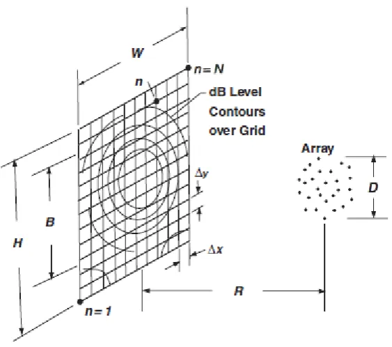
distinction in mathematical terms, the term ’beamwidth’ is introduced. The beamwidthBis defined as the diameter of the 3dB down output of the beam-form map, compared to its maximum. For convential beambeam-forming

B≈C( R

f D) (5.12)

whereRis the distance from the array to the scanning plane,Dis the array diameter (figure5.1) andCa constant.

The parameter ration ∆x/B and W/B appear to be most important for establishing resolution and spatial extent requirements of the scanning plane. The resolution∆x/B must be fine enough such that individual grid points along with other grid points represent a reasonable physical distribution of sources. However, too fine distribution would require lots of computational effort.

On the other hand, a too coarse distribution would render solutions ofXˆ which would not show the required spatial detail.

Figure5.1[4] shows some of the above mentioned parameters.

5.4

DAMAS results

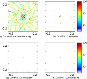
In this section some results from the DAMAS deconvolution method are shown and compared with results from conventional beamforming plots. For different frequencies and number of iterations the results will be plotted.

Figure 5.1: DAMAS geometric parameters Iterations 5000Hz 10000Hz 20000Hz

B 0.1523 0.0800 0.0400

10 80.5982 88.8046 96.0881 100 88.4683 94.9115 99.9566 1000 93.2602 99.7010 99.9977 Table 5.1: Source strength after different iteration numbers

the same experiment at 10000Hz. The results of the experiment at 20000Hz are shown by figure5.4.

-0.2 0.2 -0.2

0.2

100

(a) Conventional beamforming

-0.2 0.2

80 90 100

(b) DAMAS 10 iterations

-0.2 0.2

-0.2 0.2

(c) DAMAS 100 iterations

-0.2 0.2

80 90 100

(d) DAMAS 1000 iterations

Figure 5.2: DAMAS 5000Hz

-0.2 0.2

-0.2 0.2

100

(a) Conventional beamforming

-0.2 0.2

80 90 100

(b) DAMAS 10 iterations

-0.2 0.2

-0.2 0.2

(c) DAMAS 100 iterations

-0.2 0.2

80 90 100

(d) DAMAS 1000 iterations

-0.2 0.2 -0.2

0.2

100

(a) Conventional beamforming

-0.2 0.2

80 90 100

(b) DAMAS 10 iterations

-0.2 0.2

-0.2 0.2

(c) DAMAS 100 iterations

-0.2 0.2

80 90 100

(d) DAMAS 1000 iteraions

6. Experimental set-up

To investigate the behaviour of the beamforming algorithm when processing a line source, an experimental set-up has to be made. The line source is simulated using a line of equidistant monopoles. From these monopoles a synthetic CSM is contructed.

6.1

Coherent line source

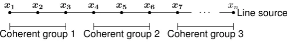
The line source is simulated using a set number of equidistant monopoles (harmonic point sources). These monopoles are added to a coherent group (see figure 6.1). All the monopoles in a coherent group are fully coherent with each other, but fully incoherent with the monopoles from other coherent groups. By varying the number of monopoles in a coherent group, different coherent lengths of the line source can be simulated.

The number of sources per length unit is the limiting factor of the lowest coherent length possible to be simulated. The length of the linesource is gives the limit of the highest coherent length possible to simulate.

6.2

Synthetic CSM

The pressure field the microphones recieve can be calculated from the su-perposition of all pressure fields of the point sources, and taking the coherent terms into account. At the construction of the CSM, only the spatial part of the sources is considered. Only considering the spatial part is equal to taking an infinite number of time averages.

6.3

Wind tunnel dimensions

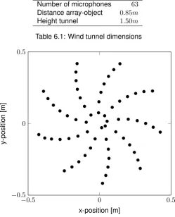
To match the computational experiments with the wind tunnel in the areo acoustic department of the University of S ˜ao Paulo, the dimensions of the wind tunnel are used for the experiments.

Line source x1 x2 x3 x4 x5 x6 x7

· · · xn

Number of microphones 63

Distance array-object 0.85m Height tunnel 1.50m Table 6.1: Wind tunnel dimensions

−0.5 0 0.5

−0.5 0 0.5

x-position [m]

y-position

[m]

Figure 6.2: 63 microphone array

6.4

Array

The array setup used is a logarithmic spiral. This setup is proven to work at low as wel as high frequency signals [5]. An overview of the array is shown in figure6.4.

6.5

Results

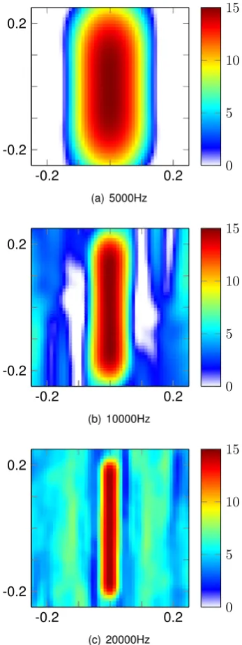
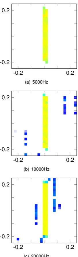
Figure 6.3shows the beamform plots of an incoherent line source. Shown is the dynamic range, from the top untill 15dB down. The plots of the other coherence lengths look the same, only the peak level (which isn’t shown in this plot) differs.

The DAMAS plots of the incoherent line source simulation are shown in figure6.4. It can be seen the sidelobes are clearly more visible in the higher freqency simulations.

-0.2 0.2 -0.2

0.2

0 5 10 15

(a) 5000Hz

-0.2 0.2

-0.2 0.2

0 5 10 15

(b) 10000Hz

-0.2 0.2

-0.2 0.2

0 5 10 15

(c) 20000Hz

-0.2 0.2 -0.2

0.2

(a) 5000Hz

-0.2 0.2

-0.2 0.2

(b) 10000Hz

-0.2 0.2

-0.2 0.2

(c) 20000Hz

7. Array Calibration Function

Experience learns the convential beamforming technique is not capable of accuratly estimating the strength of line sources. Using simulated line sources it can be noticed the peak levels of the spectral maps are sometimes a value of 15dB too high.

To cope with this problem, an array calibration function (ACF) is designed. A synthetic CSM with aline source of known strength is used for the conven-tional beamforming algorithm. The difference between beamforming output and source strength is the same for line sources of various strength levels. This difference can be used to corrigate the peak levels of wind tunnel experi-ments.

The line source is simulated with 64 equidistant monopoles, over a length of 0.4m. The use of 64 monopoles makes it possible to form multiple coherent groups, and thus simulating different coherent lenghts. The strenght of the monopoles is set at 100dB. The ACF value is the source strength minus the beamforming peak level, therefore in wind tunnel experiments, adding the ACF value to the results, gives the correct peak value.

0.2 0.4 0.6 0.8 1 1.2 1.4 1.6 1.8 2

·104

0 2 4 6 8 10 12 14 16 18 20

Frequency [Hz]

A

CF

[dB]

Monopole Incoherent

CL = 5cm CL = 10cm CL = 20cm CL = 40cm

8. Determination of

coherence levels

To use the array calibration function (chapter7) on a signal measured at wind tunnel experiments, it is required to know the coherence length of the sources in the experiment. To determine the sound coherence length, the coherence is calculated between different scanning points of the acoustic source plot. This coherence can be found by a modification of the conventional beamforming algorithm [3]. The convential beamforming algorithm is given by:

ˆ eTGˆˆe

(eˆTeˆ)2 (8.1)

For the determination of coherence levels, the beamforming algorithm is modified to use two different scanning points.

|ˆeTGˆd|ˆ2

(ˆeTGˆˆe)(dˆTGˆdˆ)

(8.2)

In this equationdˆis the steering vector for a second scan point. This way the coherence level between two different points can be calculated. If one of these points is kept as a reference point, and the other is varied over the grid, coherence plots can be made.

8.1

Incoherent monopoles

This method is first used on a simulation with two incoherent monopoles. The results of this simulation are given in figure 8.1. The first monopole source is marked with an X, and is also the reference point. The second monopole source is a mirror of the first source over they-axis.

It can be seen that when scanning frequency increases and thus beamwidth decreases, the source distribution becomes more visible. For the low frequen-cies (1500Hz and 2000Hz), the scanning resolution is too low to distinguise the two different sources. For higher frequencies the different sources can be seen.

The high coherence levels around the two sources are due to the fact that sidelobes, although they have a low level in the conventional source plot, are fully coherent with the original source. This indicates that the coherence plots may be used to identify sidelobes in acoustic source plots [1].

8.2

Line source

-0.2 0.2 -0.2

0.2

(a) 1500Hz

-0.2 0.2

(b) 2000Hz

-0.2 0.2 0

0.2 0.4 0.6 0.8 1

(c) 3500Hz

-0.2 0.2

-0.2 0.2

(d) 5000Hz

-0.2 0.2

(e) 7500Hz

-0.2 0.2 0

0.2 0.4 0.6 0.8 1

(f) 10000Hz

Figure 8.1: Coherence plots for different scanning frequencies

a frequency of 5000Hz. The results of the 10000Hz simulation are shown in figure8.3. Figure8.4shows the 20000Hz simulation results.

-0.2 0.2 -0.2

0.2

(a) Incoherent

-0.2 0.2 0

0.2 0.4 0.6 0.8 1

(b) 5cm

-0.2 0.2

-0.2 0.2

(c) 10cm

-0.2 0.2 0

0.2 0.4 0.6 0.8 1

(d) 20cm

Figure 8.2: Coherence plots 5000Hz

-0.2 0.2

-0.2 0.2

(a) Incoherent

-0.2 0.2 0

0.2 0.4 0.6 0.8 1

(b) 5cm

-0.2 0.2

-0.2 0.2

(c) 10cm

-0.2 0.2 0

0.2 0.4 0.6 0.8 1

(d) 20cm

-0.2 0.2 -0.2

0.2

(a) Incoherent

-0.2 0.2 0

0.2 0.4 0.6 0.8 1

(b) 5cm

-0.2 0.2

-0.2 0.2

(c) 10cm

-0.2 0.2 0

0.2 0.4 0.6 0.8 1

(d) 20cm

9. Conclusion

During this internship period information is gained on the behaviour of acoustic source plots generated by beamforming and DAMAS algorithms. It is found that when investigating source strength by using peak levels, the levels are not giving the right results. The value of this off result differs for various coherence lengths.

Since DAMAS deconvolution method peak levels converge to the peak lev-els of conventional beamforming, the off result of both methods is the same.

An array calibration function is made, which calibrates the peak levels of conventional beamforming and DAMAS, to give no off result. The ACF is in-dependant of source strength and number of sources used to simulate a line source. Coherence length and frequency are the two variables.

To extract coherence length from experimental results a modified beam-forming algorithm is used. This method however, does not give absolute cer-tainty about the coherence length. Since the coherence length of experimental results is not absolutely sure, the wrong calibration curve of the ACF can be picked, which can lead to an error up to 2dB.

The ACF and coherence lenght extraction method aren’t tested on exper-imental results, since no experexper-imental data was available at the time. For further research it is recommended to test both methods on experimental data for validation purposes.

9.1

Postscript

This internship period has been a valuable experiance. Good insight in the ac-tivities involved in experimental research is obtained. A lot has been learned on beamforming characteristics and working with high end wind tunnel equip-ment.

B

IBLIOGRAPHY

[1] S. Oerlemans & P. Sijtsma, Determination of absolute levels from phased array measurements using spatial source coherence. AIAA paper 2002-2464 2002.

[2] Kjell J. G ˚asvik, Optical Metrology, third edition. West Sussex: John Wiley & Sons Ltd. 2002.

[3] Horne, C., Hayes, J.A., Jaeger, S.M., and Jovic, S., Effects of dis-tributed source coherence on the response of phased arrays, AIAA paper 2000-1935, 2000.

[4] Brooks, T.F. and Humphreys, W.M., A deconvolution approach for the map-ping of acoustic sources (DAMAS) determined from phased microphone arrays, Journal of Sound and Vibration 294, 2006.