Friedman and Divisia Monetary Measures

Friedman and Divisia Monetary

Measures

william, barnett

University of Kansas

16 December 2013

Online at

https://mpra.ub.uni-muenchen.de/52310/

Friedman and Divisia Monetary Measures

William A. Barnett

University of Kansas, Lawrence, Kansas

Center for Financial Stability, New York City

IC

Institute, University of Texas at Austin

Abstract

:

This paper explores the relationship between Milton Friedman’s

work and the work on Divisia monetary aggregation, originated by William

A. Barnett. The paradoxes associated with Milton Friedman’s work are

largely resolved by replacing the official simple-sum monetary aggregates

with monetary aggregates consistent with economic index number theory,

such as Divisia monetary aggregates. Demand function stability becomes

no more of a problem for money than for any other good or service.

Money becomes relevant to monetary policy in all macroeconomic

traditions, including New Keynesian economics, real business cycle theory,

and monetarist economics.

Research and data on Divisia monetary aggregates are available for

over 40 countries throughout the world from the online library within the

Center for Financial Stability’s (CFS) program, Advances in Monetary and

Financial Measurement. This paper supports adopting the standards of

monetary data competency advocated by the CFS and the International

Monetary Fund (2008, pp. 183-184).

Keywords

: Divisia monetary aggregates, demand for money, monetarism,

index number theory.

Contributor Biography

:

William A. Barnett is the Oswald Distinguished

Professor at the University of Kansas, Director of the Center for Financial

Stability in NY City, and Senior Research Fellow at the IC

Institute of the

University of Texas at Austin. He is Founder and Editor of the Cambridge

University Press journal,

Macroeconomic Dynamics

, and the Emerald Press

monograph series,

International Symposia in Economic Theory and

Econometrics

. He is the Founder and President of the Society for

Friedman and Divisia Monetary Measures

William A. Barnett

“This [simple summation] procedure is a very special case of the more general approach. In brief, the general approach consists of regarding each asset as a joint product having different degrees of ‘moneyness,’ and defining the quantity of money as the weighted sum of the aggregated value of all assets, the weights for individual assets varying from zero to unity with a weight of unity assigned to that asset or assets regarded as having the largest quantity of ‘moneyness’ per dollar of aggregate value. The procedure we have followed implies that all weights are either zero or unity.

The more general approach has been suggested frequently but experimented with only occasionally. We conjecture that this approach deserves and will get much more attention than it has so far received.”

[Friedman and Schwartz, (1970, pp. 151—152)]

1. Introduction

The fact that simple sum monetary aggregation is unsatisfactory has long

been recognized, and there has been a steady stream of attempts at weakening the

implied perfect substitutability assumption by constructing weighted average

monetary aggregates. See, for example, Hawtrey (1930), Gurley (1960, p. 7—8),

Friedman and Meiselman (1963, p. 185), Kane (1964), Ford and Stark (1967),

Chetty (1969, 1972), Friedman and Schwartz (1970 p. 151—52), Steinhauer and

Chang (1972), Lee (1972), Bisignano (1974), Moroney and Wilbratte (1976), and

Barth, Kraft, and Kraft (1977).1

Since those weighted averages were not directly based upon aggregation or

index number theory, there is a continuum of such potential “ad hoc” weighting

1 _{Belongia (1995) provides a survey of work on weighted monetary aggregates.}

schemes, with no basis in economic theory to prefer one over the others.

Economic aggregation and index number theory were first applied to monetary

aggregation by Barnett (1980), who constructed monetary aggregates based upon

Diewert’s (1976) class of ‘superlative’ quantity index numbers with user cost

pricing. Barnett’s 1980 paper, formally derived from intertemporal economic

optimization theory, marks the beginning of modern monetary aggregation theory.

Since simple sum aggregation is clearly inappropriate at high levels of

aggregation, most economists have rarely placed much faith in the broader

aggregates. An exception was Milton Friedman, who rejected M1 and became a

strong advocate of M2. Nevertheless, Friedman and Schwartz, (1970, pp. 151-152)

clearly described the problem with high level simple sum aggregates in the

quotation at the top of this article.

I had not been aware of that quotation, when I published my 1980 paper. I

found out from a surprising phone call. Shortly after the paper appeared, I

received a phone call from my old friend, Arnold Zellner, at the University of

Chicago. He told me that he had had lunch with Friedman at the Hoover

Institution, and Friedman wanted Zellner to ask me to cite the above quotation

from the Friedman and Schwarz book. I do not know why Friedman felt the need

for a middle man. He could have called me directly, and I would have been more

than happy to cite him on the subject. Clearly Friedman and Schwartz had

In fact, there is a long footnote to that quotation, listing many of Friedman’s

students who had worked on that problem in their dissertations at the University

of Chicago. Evidently trying to solve that problem was a major issue in the

well-known monetary workshop for his PhD students. The fact that they had not been

able to solve the problem was not a result of lack of focus or will.2 _{The reason was}

that the user cost price of monetary assets had not yet been derived until Barnett

(1978) published his derivation, and the gap between index number theory and

aggregation theory had not yet been closed, prior to Diewert’s (1976) work on

superlative index numbers, unifying aggregation and index number theory.

Nevertheless, Friedman had anticipated the nature of the user cost price of

monetary assets in his classic work, Friedman (1956), in which he recognized the

relevancy of the opportunity cost of holding money and the fact that velocity is not

a constant but rather depends upon interest rates. This correct conclusion was a

break from the early Cambridge equation approach, which postulated a constant

velocity. But for policy purposes, he advocated focusing only on the long run,

under the assumption that the interest rate on capital is at its nearly constant

“natural level.” Hence for Federal Reserve policy, he did advocate the Cambridge

equation, depending only on permanent income, with the velocity function

evaluated with its arguments set at their long run natural values, viewed as

constant. He argued that interest rate and velocity variations over the business

2 _{They had recognized that money is a joint product in Friedman and Schwartz (1969).}

cycle were normal parts of the economy’s transient response and should not

motivate attempts at countercyclical policy, which he viewed as often

counterproductive, because of long lags in policy response and in the transmission

mechanism.

When I derived the foundations of modern monetary aggregation and index

number theory and began computing and supplying the Divisia monetary

aggregates, I was on the staff of the Federal Reserve Board. I had the tools

available that I needed. While Friedman and his students were ahead of their time

in their focus, they did not have the tools they needed.

Of course I was very flattered that Friedman would want me to cite his

work as supporting mine and as showing how much time and effort he and his

students had put into trying to solve the problem. In Barnett (1982) I cited

Friedman and Schwartz (1970) and provided the above quotation. I also have

done so repeatedly in subsequent publications, such as Barnett and Serletis (2000,

p. 127), Barnett and Chauvet (2011a, p. 11; 2011b, p. 18), and Barnett (2012, p.

44).

Friedman was often criticized for his skeptical views about the Federal

Reserve, even when he was visiting at the Federal Reserve. While I was on the staff

of the Federal Reserve Board, I heard how this developed. He was on the

semiannual panel of economic advisors to the Federal Reserve Board. At one

never returned. The Federal Reserve would have liked him to continue in that roll,

since as a critic he was viewed far more favorably than Karl Brunner, who was

really disliked. The guards at the entrances to the Federal Reserve building were

given orders never to permit Brunner in the building. There were no such orders

to keep out Friedman, but he never did return.

I have a somewhat unusual view of Friedman’s criticisms of Federal

Reserve policy. I do not believe that he was too distrustful of the Federal Reserve.

On the contrary, I argue that his occasional misjudgments on monetary policy were

caused by excessive trust in the Federal Reserve. He regularly reached conclusions

based on the Federal Reserve’s official simple sum monetary aggregates, which he

should not have trusted.

In contrast, during an airport conversation, I asked Brunner whether he

was upset about being barred from the Federal Reserve Board building. He smiled

at me, and said, “Bill, nothing has done more for my career.”

2. The Problem

By equally weighting components, simple sum aggregation can badly

distort an aggregate. If one wished to obtain an aggregate of transportation

vehicles, one would never aggregate by simple summation over the physical units,

of, say, subway trains and roller skates. Instead one could construct a quantity

index using weights that depend upon the valuesof the different modes of

measured by the Federal Reserve’s former broadest simple-sum aggregate, L. It

included most of the national debt of short and intermediate maturity. All of that

debt could be monetized (bought and paid for with freshly printed currency)

without increasing either taxes or L, since the public would simply have exchanged

component securities in L for currency.However, the Divisia index over the

components of L would not treat this transfer as an exchange of ‘pure money’ for

‘pure money.’ Instead Divisia L would likely rise at about the same rate as the

inflation in prices that would result from this action. In short, Divisia L would

behave in a manner consistent with Friedman’s frequently published views about

the neutrality of money, while simple sum L would not.

At the opposite extreme, many problems associated with policies that target

low level aggregates, such as M1, result from the inability of those aggregates to

internalize pure substitution effects occurring within the economy’s transactions

technology, because the aggregation is over such a small subset of the factors of

production in that transactions technology. Friedman’s early rejection of M1 is

consistent with that theory.

The traditionally constructed high level aggregates (such as M2, former M3,

and former L) implicitly view distant substitutes for money as perfect substitutes

for currency. Rather than capturing only part of the economy’s monetary services,

as M1 does, the broad aggregates swamp the included monetary services with

aggregate that captures the contributions of all monetary assets to the economy’s

flow of monetary services.

3. The Divisia Quantity Index

3.1. The Definition

In this section, I define the Divisia monetary quantity index and describe

the procedure for computing it.

Before the Divisia index formula can be computed, the user cost price of

each component monetary asset must be computed, since the price of the services

of a durable, such as money, is its user cost. The complete formula for the user cost

price of a monetary asset was derived in Barnett (1978, 1980). However, a

simplification is possible. All of the factors in the formula for the ith asset’s user

cost, πi, can be shown to cancel out of the Divisia index except for R−ri, where for

any given time period, ri is the own rate of return on asset i and R is the expected

maximum holding period yield available in the economy during that period.

The growth rate of the Divisia quantity index is a weighted average of the

growth rates of the component quantities. _{The weights are the corresponding}

user-cost-evaluated value shares. Since those value shares represent the

contributions of the components to expenditure on the services of all of the

quantity growth rates makes intuitive sense but are derived from a formal

mathematical proof, not from ad hoc economic intuition.3

It is important to recognize that the user costs are not the weights, but

rather are the prices used along with all of the quantities in computing the weights.

Each weight depends upon all prices and all quantities. _{In fact, if the own price}

elasticity of demand of asset i is greater than one, then changes in the asset’s own

rate of return will induce changes in the asset’s weight in the same direction. In

the case of Cobb-Douglas utility, the expenditure shares, and therefore the Divisia

growth rate weights, are independent of prices, while in general the direction in

which the weights move, when own interest rates move, depends upon whether

the own price elasticity of demand is greater than or less than 1.0.

In addition, it is important to recognize that the shares are not weights on

levels, but on growth rates. Solving the Divisia differential equation for the level of

the aggregate shows that levels of aggregates are deeply nonlinear line integrals

and cannot be expressed as weighted averages of component levels. Most

misunderstandings of the Divisia monetary aggregates result from lack of

understanding of that fact.

It can be shown that the simple sum aggregates are a special case of the

Divisia aggregates. If all own rates of return on all monetary assets are the same,

then the growth rates of the Divisia indices reduce to the growth rates of the

3 _{For a presentation of the general theory of Divisia aggregation, see Balk (2005; 2008, chapter 6).}

corresponding simple sum aggregates. _{The implied assumption of always equal}

own rates could be justified, if all component monetary assets were perfect

substitutes. In fact, many decades of accumulated empirical research, reported in

the published literature, overwhelmingly suggest that substitutability among

different monetary assets is low,and of course all component own rates of return

are not the same, except when all interest rates have been driven down to the zero

rate of return on currency. In short, simple sum monetary aggregation can be

justified as an approximation, only when financial markets are in a liquidity trap,

as has been the case in the United States during and immediately after the Great

Recession.4

3.2. The Effects of Interest Rate Changes

If the interest rate on a component monetary asset is changed (resulting in

a change in the user cost), asset holders will respond by substituting towards the

assets with relatively decreased user costs (i.e., increased own yield). The Divisia

monetary quantity index will change only if the approximated economic quantity

aggregate changes. The economic quantity aggregate can be a utility, distance, or

production sub-function, such as a transactions technology, weakly separable from

the economy’s structure, to satisfy the theoretical existence condition for an

aggregator function. Hence the aggregate will change only if the change in relative

4 _{By “liquidity trap,” I mean a situation in which nominal interest rates are near their lower bound}

of zero. I do not mean to suggest that the central bank loses its ability to influence liquidity, when interest rates are near zero. The latter was shown not to be the case by Brunner and Meltzer (1968).

prices results in a change in the aggregator function, or, equivalently, in the

monetary asset service flow, as perceived by the economic agent. Equivalently, the

index number will change only if the change in the interest rate has an income

effect. Any quantity index number constructed from index number theory will

perfectly internalize pure substitution effects, which, by definition, occur at

constant levels of monetary service flows. Hence, the aggregate will notchange,

when it shouldnotchange. The simple sum aggregate, on the other hand, does not

internalize pure substitution effects. Interest rate changes cause shifts in a simple

sum aggregate, even when there has been no change in monetary service flows.

The conclusions reached in the previous paragraph are produced by

economic index number theory. But it should be observed that the exact same

Divisia monetary index can be acquired without the use of economic theory. The

statistical theory of index numbers, advocated by Henri Theil (1967) and others,

can produce the same index from stochastic reasoning.5 _{In short, the expenditure}

shares, which are all between 0 and 1, are viewed as probabilities, and the index’s

growth rates are produced as a statistical mean of the component growth rates

with those probabilities. The resulting Divisia index is then interpreted in terms of

statistical sampling theory.

5 _{See Barnett and Serletis (2000, pp. 172-173).}

4. Graphical Comparisons of the Divisia and Simple Sum Aggregates

The extensive available graphical comparisons between the behavior of the

Divisia and simple sum monetary aggregates are scattered over various sources. In

this section, some of the more interesting graphical comparisons from those

sources are collected together and discussed relative to the views of Milton

Friedman.

The first charts of the behavior of the Divisia aggregates appeared in

Barnett (1980) and Barnett and Spindt (1979). One of those charts is reproduced

below as Figure 1. That figure contains plots of the velocity of the Federal

Reserve’s former M3 and of M3+_{, which roughly corresponds to the aggregate later}

called L and now called M4 by the Center for Financial Stability in New York City.

Velocity is plotted in each of those cases with the monetary aggregate alternatively

computed as a simple sum or as a Divisia quantity index. With M3+ _{the Laspeyres}

quantity index also is used. These figures are of particular importance, since they

focus on the years that produced the view of money demand structural breaks and

instability, with particular emphasis on 1974.

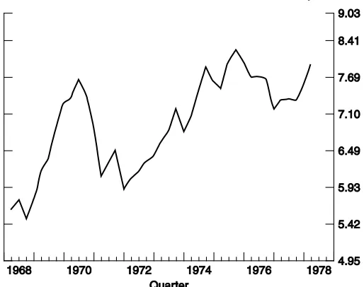
The velocity of the Divisia aggregates can be seen to follow a path that

closely resembles that of the interest rate cycle from 1968 to 1978, as displayed in

Figure 2. Hence velocity appears to be a stable function of the opportunity-cost

interest rate. In addition, the Laspeyres quantity index moves much more closely

simple sum aggregates can be seen to trend downwards in a manner that violates

theoretical views regarding the behavior of velocity during periods of rising

interest rates and inflationary expectations. Substitution between money and

higher yielding assets (disintermediation) appears to go in the wrong direction.

Figure 1: Seasonally adjusted normalized velocity during the 1970s.

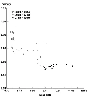
Most of the concern about economic “paradox” in the 1970s was focused on

1974, when it was believed that there was a sharp structural shift in money

markets in the form of a shift that could not be explained by interest rate

movements. Figure 3 displays a source of that concern, taken very seriously by the

Federal Reserve Board staff at that time. In figure 3, we have plotted velocity

against a bond rate, rather than against time. As is evident from Figure 3, there

appears to be a dramatic shift downwards in velocity in 1974, and clearly that shift

cannot be explained by interest rates, since it happened suddenly at a time when

there was little change in interest rates. But observe that this result was acquired

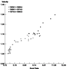
using simple sum M3. Figure 4 displays the same cross plot of velocity against an

interest rate, but with M3 computed as its Divisia index. Observe that velocity no

longer is constant, either before or after 1974. But there is no structural shift,

since the variations in velocity correlate with interest rates. In fact the plot not

only has no discontinuous jump at a particular interest rate, but is nearly along a

straight (linear) line. Also note that the line slopes in the correct direction:

velocity goes up when interest rates go up, as is consistent with demand for money

Figure 4: Divisia M3 velocity versus interest rate: Moody’s AAA corporate bond rate, quarterly, 1959.1-19980.3

At that time, the claims of unstable demand for money and unstable velocity

function, both denied by Milton Friedman, grew in influence. Milton Friedman was

right, as was known by the Federal Reserve Board’s model manager, Jerry Enzler,

but was not revealed to the public. The hypothesis was tested carefully by PAVB

Swamy and Peter Tinsley on the Federal Reserve Board’s staff. They produced a

stochastic coefficient model of the Goldfeld (1973) money demand equation, used

at that time in the published research on unstable money demand and used in the

Board’s macroeconometric model. Swamy and Tinsley ran the test twice: once

hand side. No changes were made to the right hand side of that equation. The

conclusion was that money demand was unstable with simple sum money but

stable with Divisia money. See Barnett, Offenbacher, and Spindt (1984). These

results were known to Jerry Enzler.

About a year after I had left the Federal Reserve Board’s staff for my first

academic position, at the University of Texas at Austin, I received an astonishing

telephone call from a former Federal Reserve Board staff economist. He informed

me that Jerry Enzler had had a serious automobile accident and was on permanent

disability leave. His replacement discovered that Jerry had changed the official

simple sum M2 aggregate to the corresponding Divisia M2 aggregate in the Board’s

quarterly macroeconometric model. Jerry had told no one that he had made that

change. More information about those events can be found in my book, Barnett

(2012).

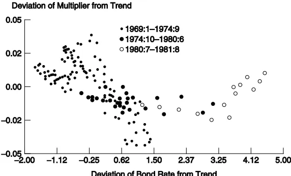
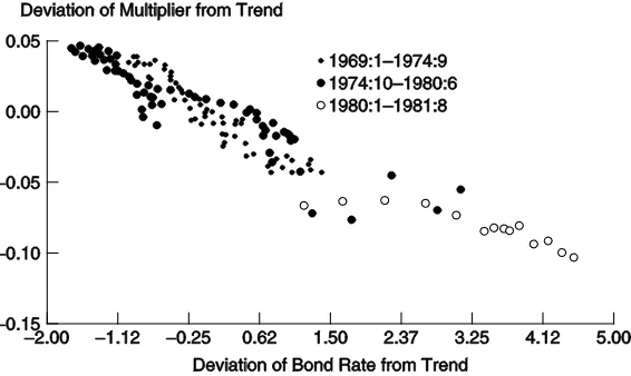
There were analogous concerns about the supply side of money function.

The reason is evident from Figure 5, which plots the base multiplier against a bond

rate’s deviation from trend. The base multiplier is the ratio of a monetary

aggregate to the monetary base. There is good reason for looking at that ratio. The

Federal Reserve’s open market operations change the Federal Reserve’s balance

sheet. Those changes, in turn, change the “monetary base,” also called “high

powered money,” or outside money. Changes in the monetary base work

supply. That was viewed as a “transmission mechanism” for monetary policy to

the money supply, and thereby to inflation and the economy. The ratio of the

money supply to the monetary base should exceed 1.0, since bank reserves back a

larger amount of bank deposits by customers, since only a fraction of the total

deposits need be held as reserves. The controllability of the money supply was

viewed as depending heavily upon the ability to anticipate the ratio of the money

supply to the monetary base. That ratio, also called a “multiplier,” need not be

constant to assure controllability of the money supply, but should best be stably

related to interest rates, so the multiplier can be anticipated based upon current

interest rates. It was believed that open market operations then could be used to

influence the money supply through changes in the monetary base, which is

directly under the control of the Federal Reserve through its open market

operations.

In Figure 5, the monetary aggregate is again the simple sum M3, as

computed and officially provided by the Federal Reserve at that time. The base

multiplier (adjusted for trend) is plotted against an interest rate. Observe the

dramatic structural shift, which is not explained by interest rates. Prior to 1974,

the data are along a curved line, in fact a parabola. After 1974 the data is along an

intersecting straight line. But again this puzzle was produced by the simple sum

monetary aggregate. In Figure 6, the same plot is provided, but with the monetary

A systematic comparison of Divisia versus simple sum monetary

aggregation during those years of growing skepticism about money demand

stability was conducted initially by Barnett, Offenbacher, and Spindt (1984) and

subsequently, over a longer time span, by Belongia (1996), who wrote in his paper’s

abstract:

“Inferences about the effects of money on economic activity may depend

importantly on the choice of a monetary index because simple-sum aggregates

cannot internalize pure substitution effects. This hypothesis is investigated by

replicating five recent studies that have challenged an aspect of the 'conventional

wisdom' about the effects of money on aggregate activity. In four of the five cases,

the qualitative inference in the original study is reversed when a simple-sum

monetary aggregate is replaced by a Divisia index of the same asset collection.”6

Figure 5: Simple-sum M3 base multiplier versus interest rate: deviation from time trend of Moody’s

Baa corporate bond rate, monthly 1969.1-1981.8.

6 _{Hendrickson (2013) reached similar conclusions in replications of published}

studies, but with the simple sum aggregates replaced by the comparable Divisia measures.

5. End of the Monetarist Experiment: 1983-1984

As stated above, Friedman was not overly critical of the Federal Reserve, but

rather too trusting of the Fed’s data. In contrast, his successor at the University of

Chicago, Robert Lucas (2000, p. 270) wrote, “I share the widely held opinion that

M1 is too narrow an aggregate for this period, and I think that the Divisia approach

offers much the best prospects for resolving this difficulty.” Particularly puzzling

was Friedman’s continued confidence in Federal Reserve monetary aggregates

following the end of the Monetarist Experiment.7 _{At that time, he became very}

vocal with his prediction that there had just been a huge surge in the growth rate

of the money supply, and that the surge would work its way through the economy

to produce a new inflation. He further predicted that there would subsequently be

an overreaction by the Federal Reserve, plunging the economy back down into a

recession. He published this view repeatedly in the media in various magazines

and newspapers, with the most visible being his Newsweek article, “A Case of Bad

Good News,” which appeared on p. 84 on September 26, 1983. I have excerpted

some of the sentences from that Newsweek article below:

“The monetary explosion from July 1982 to July 1983 leaves no satisfactory way out

of our present situation. The Fed’s stepping on the brakes will appear to have no

immediate effect. Rapid recovery will continue under the impetus of earlier

monetary growth. With its historical shortsightedness, the Fed will be tempted to

step still harder on the brake – just as the failure of rapid monetary growth in late

7 _{Other puzzles include Friedman's inconsistent switches between simple sum M1 and}

M2 during 1981-1985, when offering policy prescriptions and critiques, as documented in Nelson’s (2007, pp. 162-166) history of Friedman's views.

1982 to generate immediate recovery led it to keep its collective foot on the

accelerator much too long. The result is bound to be renewed stagflation – recession

accompanied by rising inflation and high interest rates . . . The only real uncertainty

is when the recession will begin.”

But on exactly the same day, September 26, 1983, I published a very different view

in my article, “What Explosion?” on p. 196 of Forbes magazine. The following is an

excerpt of some of the sentences from that article:

“People have been panicking unnecessarily about money supply growth this year.

The new bank money funds and the super NOW accounts have been sucking in

money that was formerly held in other forms, and other types of asset shuffling also

have occurred. But the Divisia aggregates are rising at a rate not much different from

last year’s . . . the ‘apparent explosion’ can be viewed as a statistical blip.”

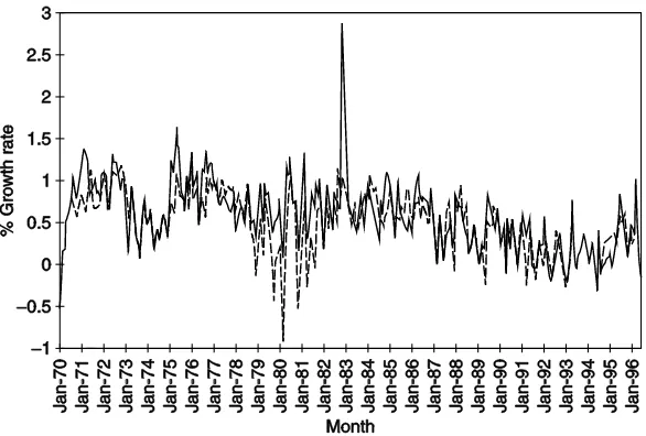
Milton Friedman would not have taken such a strong position without reason.

His reason is evident from Figure 7, acquired from the St. Louis Fed’s web site.8

The percentage growth rates in that figure are not annualized, so should be

multiplied by 12 to acquire the approximate annualized growth rates. Notice the

large spike in growth rate, which increases to nearly 36% per year. But that solid

line is produced from simple sum M2, which was greatly overweighting the sudden

new availability of super-NOW accounts and money market deposit accounts.

There was no spike in the Divisia monetary aggregate, represented by the dashed

line.

8 _{The St. Louis Federal Reserve Bank has played a historic role in supplying Divisia monetary}

aggregates for the United States. See Anderson and Jones (2011). A newer source, including broad Divisia monetary aggregates, is the Center for Financial Stability in New York City. See Barnett, Liu, Mattson, and van den Noort (2013) and http://centerforfinancialstability.org.

If the huge surge in the money supply had happened, then inflation would

surely have followed, unless money were extremely non-neutral even in the long

run --- a view held by very few economists. But there was no inflationary surge

and no subsequent recession.

Subsequent to the work of Friedman on monetary economics, there has been

a dramatic increase in substitutes for money associated with “shadow banking.”

Long before the evolution of shadow banking assets, Keynes recognized the

relevancy of broad monetary measures.9 _{Paradoxically, the response of the}

Federal Reserve to money market innovations has been to remove the entire

negotiable money market from its monetary aggregates, by discontinuing its broad

aggregates, M3 and L, since simple sum aggregation over substitutes for money

excessively weight substitutes for money. In contrast, Divisia monetary aggregates

can dynamically incorporate properly weighted substitutes for money as they

evolve, and as made available to the public by the Center for Financial Stability in

its broadest monetary aggregates, M3 and M4.

9 _{Given that the assets in the Keynes (1936) model consisted of just aggregated money and}

aggregated bonds, it is hard to think that he conceived of the relevant aggregate as anything but a broad one. That conclusion would also be consistent with his discussion of the role of what he called "the financial circulation" in Keynes (1930). On this point, also see Tim Congdon (2011, pp. 28 and 83). I am indebted to David Laidler for pointing this out to me.

Figure 7: Monetary Growth Rates, 1970-1996, from St. Louis Federal Reserve’s Database, FRED. The growth rates are not annualized.

6. Optimal Aggregation

Having briefly surveyed the source of misunderstandings about money

demand and money supply, I now outline the formal procedure for correct

monetary aggregation, as consistent with the fields of index number and

aggregation theory and with Barnett (1982). In economic theory, the optimal

aggregate is acquired through a three-stage selection procedure. The selection

procedure at each stage is distinct and the stages cannot be interchanged in order.

As we shall see, the deficiencies in the official aggregates result from the fact that

the third-stage criteria alone have been used to select the aggregates, although

those criteria are inappropriate within either of the two prior stages.

The first stage in the selection of an optimal aggregate is the determination

of all theoretically admissible sets of components assets. Aggregates then can be

constructed over only those sets. To acquire those admissible sets, we first must

acquire the separable subsets of the set of all monetary components.

We now define the conditions for a separable subset, which we shall call a

separable component group.

Condition 1: Let C be a subset of the set of all monetary assets, M, so that C

is itself a set of component monetary assets. Then C is a separable component

group, if and only if the marginal rate of substitution between any two assets in C is

independent of the quantity of any good or asset not in C.

Condition 1 is necessary and sufficient for a subfunction of the assets in C

alone to be factorable out of utility or production functions. The value of that

factored subfunction, which is called the economic aggregate, depends only upon

the assets in C and is independent of the quantities consumed or held of any other

goods or assets. Without condition 1, no stable preferences or transactions

technology can exist over elements of C alone, and hence goods or assets not in C

will act as missing shift variables in the demand for any aggregates constructed

over assets in C alone.

We call condition 1 the Existence Condition, since it defines the condition

under which an economic aggregate exists in aggregation theory. However,

good. To acquire that result, we need the following stronger condition, which we

call the Consistency Condition.

Condition 2. An admissible component group, C, is a consistent component

group, if the elasticity of substitution between any component asset in the group

and any good or asset not in the group is independent of the good or asset that is

not in the group.10

Condition 2 implies condition 1, but the converse is not true. Every

consistent component group is separable, but not every separable component

group is consistent. Although some aspects of aggregation theory can be applied

with only satisfaction of condition 1, condition 2 substantially simplifies

interpretation and use of an aggregate.11 _{Condition 2 is acquired by imposing}

linear homogeneity on the economic aggregate that condition 1 assures exists over

the assets in C. It would be very curious indeed if linear homogeneity of an

aggregate failed; in such a case, the growth rate of the aggregate would differ from

the growth rates of the components, even if all components were growing at the

same rate.

Neither condition 1 nor condition 2 has meaning unless the concept of

substitutability among assets has meaning. We need the existence of a utility

function or production function containing monetary assets (with or without other

goods) as arguments. The existence of a transactions technology would suffice.

10 _{Condition 2 defines a linearly homogeneous, weakly separable block in aggregation theory.} 11 _{Examples using only condition 1 can be found in Barnett (1980) and Barnett (1981, chap. 7).}

If our objective were to explain why people hold money, then entering

monetary assets enter utility or production functions would be assuming away the

problem. However for our purposes, we can assume that money has positive value

in equilibrium. Under that assumption, it has been proved in general equilibrium

theory that money must enter into a derived utility or production function.12

Hence conditions 1 and 2 can be defined relative to that derived function.13

In order for an aggregate to serve the role of ‘money’ in the economy, we

would expect the components to satisfy another restriction. In addition to

satisfying condition 2, the components should satisfy the following condition,

which we call the Recursiveness condition.14

Condition 3. The components of each aggregate must include currency (legal

tender) and must not include any good or asset that is not a ‘monetary asset.’

Although aggregation theory provides no definition of ‘monetary asset,’ the

identity of the ‘money market’ is no less widely understood than the identity of the

durables market or the recreational goods market. In attaching a name to an

12 _{See Arrow and Hahn (1971) and Quirk and Saposnik (1968, p. 97). A widely used special case of}

the general equilibrium result arises if money acquires its usefulness by entering a transactions constraint. In that case the derived utility function is the Lagrangian containing both the original elementary utility function (which does not contain money) and the constraint defined by the transactions technology. See Phlips and Spinnewyn (1982), whose approach applies regardless of whether money does or does not yield interest.

13 _{There is still the problem of aggregating over individual economic agents (households and firms).}

For a survey of that literature, see Barnett (1981, pp. 306-7). For a newer approach to the problem, see Barnett (1979). For a well-known directly relevant approach, see Muellbauer (1975) and Phlips and Spinnewyn (1982). For recent surprisingly favorable empirical results on aggregation over economic agents, see Varian (1983).

14 _{The condition results in a recursively nested functional structure for the aggregator function in}

aggregate, such as food or money, a prior definition of the components’ domain

must be selected.

Aggregation theory itself does not dictate use of condition 3. In principle,

we would lose nothing by dropping condition 3. However in practice the number

of component groups that would satisfy condition 2 is likely to be large. Although

the condition 2 component groups would always contain the ‘best’ group (or

groups) for any particular purpose, the empirical research needed to choose

among such a large class of component groups could be difficult and expensive.

Condition 3 applies conventional views from monetary theory to restrict further

the number of admissible component groups. In particular, condition 3 restricts

the domain of possible components to ‘monetary assets’ and requires the

collection of admissible component groups to be nested about ‘hard core money,’

defined here by its legal tender property. Researchers applying the procedures

outlined in this paper could tighten or loosen the restrictiveness of condition 3 as

needed to accommodate the scope (i.e., ambitiousness) of the research, with the

limiting (most ambitious) case being elimination of condition 3 entirely.

The component groups that satisfy both conditions 2 and 3 comprise a

family of completely nested sets. Hence aggregation is perfectly recursive as we

pass to increasingly high levels of aggregation over those nested groups. We shall

call a set of components that satisfies both conditions 2 and 3 a consistent recursive

When we seek an aggregate to serve the role of ‘money’ in the economy, as

would be acquired for a monetary target or for the variable ‘money’ in a model, we

shall require the components of the aggregate to comprise a consistent recursive

component group. If we were seeking only an indicator, the prior imposition of

condition 3 would generally not be justified, and we could perhaps even do

without condition 2. We therefore say that a set of components that is separable is

admissible for an indicator.15 _{We define a set of components that is also consistent}

and recursive to be admissible for a monetary variable. Since the primary objective

of this paper is determination of the optimal monetary variable, indicators will not

be explored in detail. In the monetary asset case, I derived the precise test for

condition 2 in Barnett (1980) and in Barnett (1981, chap. 7).16

I summarize the results of this section with a statement of the solution to

the stage 1 problem in monetary aggregation:

Step 1. Determine those sets of monetary assets that satisfy both conditions

2 and 3.

15 _{For further discussion on the subject of monetary indicators, see Brunner and Meltzer (1967,}

1969) and Hamburger (1970).

16 _{The component groups used in constructing the Federal Reserve Board’s official monetary}

aggregates were not acquired by testing for either condition 1 or condition 2. Some of those component groups are probably inadmissible either for indicators or for monetary variables. For example, Series E bonds and nonnegotiable, consumer-type, small time deposits are probably not elements of any admissible monetary asset component group, although they may be elements of an admissible group of components for an intermediate-term-bond aggregate.

6.2. Stage 2: Selection of an Index Number Formula

Having determined the admissible component groupings, we next must

determine a formula to be used for computing the aggregates over the components

of each admissible group. In the Federal Reserve Board’s current official

aggregates, the formula is simple summation of the component quantities. The

aggregation formula is called the aggregator function, and the necessary and

sufficient conditions for a linear aggregator function are the following:

Condition 4. The aggregator function is linear if and only if the component

goods (or assets) are perfect substitutes.

We call condition 4 the Linearity Condition. Clearly the components of the

monetary assets are not perfect substitutes. Hence the aggregates cannot be

computed from simple summation or from any other linear formula. When

components are not perfect substitutes, a nonlinear aggregator function is needed.

The aggregate acquired from the nonlinear function is called the ‘economic

aggregate.’17

To use a nonlinear aggregator function directly, we would have to specify

the form of the function and then estimate its parameters. Alternatively index

number theory provides parameter-free approximations to the economic

aggregates of aggregation theory. Economic quantity aggregates depend upon

17 _{If mis the vector of components and if f is the aggregator function, then f(m) is the economic}

aggregate.

quantities and unknown parameters, but not prices. However quantity index

numbers depend upon quantities and prices, but not unknown parameters.

Hence quantity index numbers dispense with unknown parameters by

introducing prices. Diewert (1976) has defined the class of ‘superlative’ index

numbers, which provide very high quality approximations to economic aggregates.

In constructing a superlative monetary quantity index number, the

selection of the index number from among those in the superlative class is of little

importance, since all of the index numbers within the class move very closely

together. _{However, they all jointly diverge from the simple sum index.}

As a result, the simple sum index is entirely disreputable in the index

number literature. Fisher (1922) found that the simple sum index was the very

worst index that he was able to devise. The simple sum index was the only index

that possessed both of the bad properties that he defined: bias and freakishness,

and he found the size of the bias to exceed 35 percent of the level of the index.

Fisher (1922, p. 29) observed that “the simple arithmetic average produces one of

the very worst of index numbers, and if this book has no other effect than to lead to

the total abandonment of the simple arithmetic type of index number it will have

served a useful purpose.” Fisher (1922, p. 36) concluded that “the simple

arithmetic [index] should not be used under any circumstances.”

My work on monetary aggregates has usually applied the Divisia index

numbers in Diewert’s superlative class and hence is potentially the most useful to

policymakers.

The selection of the prices to be used in the index number formula is

important. If user cost (or “rental”) prices are used in an aggregate of durables,

such as monetary assets, then the resulting quantity index measures the service

flow generated by the component durable goods. The formula for the user cost

price of a monetary asset was derived by Barnett (1978, 1980).27

I summarize the conclusions of this section with a statement of the solution

to the stage 2 problem in monetary aggregation:

Step 2. Using user cost prices for each component asset, compute a

superlative quantity index over each of the admissible groups of component assets

acquired from step 1.

6.3. Stage 3: Selection of the Optimal Level of Aggregation

Having completed step 2, we have a hierarchy of nested aggregates. We

now must select among them.

Each element of our hierarchy of monetary quantity index numbers

approximates a perfect economic aggregate. In aggregation theory every

household and firm in the economy can be shown to behave as if a consistent

aggregate is an elementary good.18 _{Hence no information about the economy is lost}

18 _{The solution to each economic agent’s full decision is the same as the solution to a multistage}

decision. The consistent aggregates are the variables in each stage of the multistage budgeting procedure except for the last stage. The variables in the last stage are the elementary goods from the original full decision. See Green (1964, theorem 4).

by using a consistent aggregate. Since the component monetary quantities and

interest rates are not likely to be final targets of policy, we have nothing to lose by

using the highest level aggregate among those that are in the admissible hierarchy.

The question now arises as to whether we have anything to lose by using an

admissible aggregate other than the highest level aggregate, and we do indeed. By

using a lower level aggregate, we are omitting factors of production from the

economy’s transactions technology. Furthermore, as the level of aggregation

decreases, the number of price aggregates contained in the demand function

increases.19 _{As a result, modeling the demand for the aggregate becomes more}

difficult; and if any of the explanatory variables is omitted, the function will appear

to shift in an unstable fashion. However the economic aggregates of aggregation

theory can be shown to internalize pure substitution effects perfectly.

In short, the highest level admissible aggregate from step 2 provides a

properly weighted measure of the total service flow of all of the money market’s

separable components. We now can state the final step in the procedure for

choosing the optimal monetary aggregate:

Step 3. Select the highest level aggregate from among those generated by

step 2.

19 _{This result follows from duality theory. There is a price aggregate, which is dual to the quantity}

aggregate, over each group of components satisfying condition 2. The demand for automobiles depends upon the price of aggregated automobiles, fuel, and housing. But the price of BMW X3s depends upon the price of other small SUVs and individual grades of gasoline.

However, at this point it may be wise to hedge our bets. While aggregation

theory does tell us to use only the nested admissible aggregates provided by step

2, my advocacy of the highest of those aggregates on theoretical grounds depends

upon a nontrivial assumption: equilibrium in the market for every component

asset. As Cagan (1982) has observed, the economy’s disequilibrium dynamics can

affect differently the information content of aggregates at different levels of

aggregation.

Aggregates generated by step 2 at each level of aggregation will properly

measure the total service flow produced by the components, regardless of whether

interest rates are market determined or are set by regulation, and regardless of

whether the markets for components are or are not in equilibrium. Hence the

aggregates produced by step 2 remain the valid aggregate monetary variables. But

the validity of step 3 depends upon an equilibrium assumption and is therefore

conclusive only in the long run.20

The importance of the theoretical conclusion (step 3) should be an

increasing function of the weight that we place upon the objective of controlling

the long-run (equilibrium) inflation rate. I conclude this section with a statement

of the short-run disequilibrium alternative to step 3.

20 _{However it is perhaps unlikely that this problem would be serious with aggregates satisfying}

conditions 1 and 2, since the markets for those components are among the best and fastest adjusting in the economy. Nevertheless the components of the current official aggregates include some very illiquid assets having long maturities and heavy early redemption penalties. Hence until the components are properly regrouped in accordance with step 1, step 3 cannot be viewed as conclusive on theoretical grounds alone.

Step 3a. From among the admissible aggregates provided by step 2, select

the one that empirically works best in the application in which the aggregate is to

be used.

Observe that step 3a cannot be accomplished without prior completion of

steps 1 and 2. However, the Federal Reserve Board’s official aggregates are

constructed from research that related solely to step 3a. Step 1 was never

conducted, and step 2 was replaced by simple sum aggregation. As emphasized by

Mason (1976), Friedman and Schwartz (1970) contained the same violations of

scientific methodology, which insists that measurement must precede use to avoid

circularity. Nevertheless, while Friedman and Schwartz (1970) did not conduct

formal tests for blockwise weak separability of component clusterings, Swofford

(1995) did and found support for the groupings used by Friedman and Schwartz

(1970).

Step 1 is needed to assure the existence of behaviorally stable aggregates

over the component groups, and step 2 is needed to assure that the computed

aggregates provide high quality approximations to the unknown behaviorally

stable aggregates.31 _{By violating step 2, the official aggregates cannot approximate}

behaviorally stable aggregates; and by using components that need not satisfy step

1, the official aggregates permit all forms of spurious and unstable relationships

during the application of step 3a. In short, the procedure used in selecting the

replicable explanatory or predictive ability to the movements of the aggregates,

since the economy cannot act as if the official aggregates are variables in the

economy’s structure.

Movements of the official aggregates could have stable relationships with

actual structural variables, such as the inflation rate, only if the aggregates’

components were perfect substitutes, so that step 2 would be satisfied, and if step

1 were satisfied by a combination of chance and superior judgment. Clearly the

violation of step 2 is more serious than the violation of step 1, since the perfect

substitutability condition needed for satisfaction of step 2 with simple sum

aggregation could not have been satisfied by chance. In addition, if step 2 had been

applied, the possibility would have increased that the component groupings

selected from step 3a would have satisfied step 1.

7. Conclusions

Misperceptions about the stability of money demand have played a major

role in the profession’s move away from the views of Milton Friedman on

monetary policy. But current views about money demand instability are not based

on accepted methodology in the literature on consumer demand systems.

I have contributed substantially to the literature on consumer demand

systems modeling. See, e.g., the reprints of my many publications in that area in

the books Barnett and Serletis (2000), Barnett and Binner (2004), and Barnett and

seminonparametric approach (Barnett and Jonas (1983), Barnett and Yue (1988),

Barnett, Geweke, and Yue (1991)) and the Laurent series approach (Barnett

(1983)) and the generalized hypocycloidal demand model (Barnett (1977)). I am

also the originator of aggregation theoretic foundations for the Rotterdam demand

systems model (Barnett (1979)). The consumer demand modeling literature

insists upon use of microeconomic foundations along with the relevant

aggregation and index number theory. The resulting systems of equations usually

are nonlinear and estimated jointly. The views on money demand equation

instability are based on research making no use of any of the accepted

methodologies in consumer demand system modeling and estimation.

Economists working on consumer demand systems modeling are well

aware of the fact that acquiring stable systems requires state-of-the-art modeling

and estimation. My experience using that approach with money demand have

consistently shown that money demand is no more difficult to estimate stably than

demand for any other good. See, e.g., Barnett (1983). Others familiar with the

literature on modeling and estimating consumer demand systems have similarly

reached the same conclusions, over and over again for decades. See, for example,

Hendrickson (2013), Serletis (2007), and Serletis and Shahmoradi (2005, 2006,

2007). The contrary literature fails to use data or modeling approaches meeting

modeling and is thereby over a half century behind the state of the art in modeling

demand for any other good or service.

The eminent new Keynesian economist, Julio Rotemberg, has contributed in

major ways to the literature on monetary aggregation theory through his own

publications [Rotemberg (1991), Poterba and Rotemberg (1987), and Rotemberg,

Driscoll, and Poterba (1995)] and has acknowledged the following in his

endorsement quotation on the back cover of Barnett (2012): “This book first

makes you care about monetary aggregation and then masterfully shows you how

it should be done.” That book won the American Publishers Award for

Professional and Scholarly Excellence (the PROSE Award) for the best book

published in economics during 2012.

Indeed money does matters in New Keynesian models, when there are

financial shocks to the economy, as has become a major focus of research in recent

years. Keating and Smith (2013a) have shown that augmenting a typical Taylor

rule with a reaction to Divisia money growth improves welfare, when the financial

sector is a source of shocks driving the economy. This result contrasts with the

literature arguing that optimal monetary policy can be implemented in New

Keynesian models without reference to a monetary aggregate. However, that

literature makes the very strong assumption that the central bank perfectly

observes the natural rate of interest and the output gap in real time. By eschewing

realistically implementable by central banks by including the non-parametric

Divisia monetary aggregate within the policy rule.

Keating and Smith (2013b) have further shown that Friedman's constant

money growth rate rule is likely to result in indeterminacy for most parameter

values, when implemented with a simple-sum monetary aggregate. The

indeterminacy stems from simple-sum's error in tracking the true monetary

aggregate. This indeterminacy is resolved, if the rule is implemented with the

Divisia monetary aggregate. They show that a similar result is obtained when

considering inflation-targeting interest-rate rules reacting to money growth. In

particular, the addition of a reaction to simple-sum money growth creates

indeterminacy. On the other hand, inflation-targeting interest-rate rules reacting

to Divisia growth satisfy a novel type of Taylor principle --- reacting more than 1:1

to Divisia growth is sufficient for determinacy.

Belongia and Ireland (2013) similarly used a New Keynesian model in their

analysis of the potential importance of Divisia monetary aggregates in policy.21

Their paper extends a New Keynesian model to include roles for currency and

deposits as competing sources of liquidity services demanded by households.

According to their paper’s abstract,

“it shows that, both qualitatively and quantitatively, the Barnett critique

applies: While a Divisia aggregate of monetary services tracks the true

monetary aggregate almost perfectly, a simple-sum measure often behaves

21 _{Peter Ireland is a member of the Shadow Open Market Committee.}

quite differently. The model also shows that movements in both quantity and

price indices for monetary services correlate strongly with movements in

output following a variety of shocks. Finally, the analysis characterizes the

optimal monetary policy response to disturbances that originate in the financial

sector.”

Recently, many New Keynesian economists have emphasized the possible merits

of nominal GDP targeting in monetary policy. Although not necessarily advocating

nominal GDP targeting, Belongia and Ireland (2013b) and Barnett, Chauvet, and

Leiva-Leon (2013) have found that Divisia monetary aggregates should play an important role, if

nominal GDP targeting were to be adopted. Alternatively, advocates of Friedman’s

preference for monetary targeting will find support for Divisia monetary targeting in

Serletis and Rahman (2013).22

Divisia monetary aggregates are not only relevant to New Keynesian models, but

more relevant than commonly believed to classical real business cycle models, as found by

Serletis and Gogas (2014). They conclude:

“King, Plosser, Stock, and Watson (1991) evaluate the empirical

relevance of a class of real business cycle models with permanent

productivity shocks by analyzing the stochastic trend properties of

postwar U. S. data. . . . We revisit the cointegration tests in the spirit of

King et al. (1991), using improved monetary aggregates whose

construction has been stimulated by the Barnett critique. We show that

previous rejections of the balanced growth hypothesis and classical

22 _{Personally I am not an advocate of any particular policy rule, but rather of competent}

measurement within any policy approach. But I do think it paradoxical that economists favoring a monetary growth intermediate target have often preferred a simple sum monetary aggregate, while simultaneously and inconsistently preferring an inflation-rate final target measured as a chained Fisher ideal or Laspeyres index, rather than a simple sum or arithmetic average price index.

money demand functions can be attributed to monetary aggregation

issues.”

A large literature, not dependent on New Keynesian, monetarist, or real

business cycle theory, now exists on the relationship between Divisia money,

inflation, and output.23 _{In the years immediately following the Great Recession,}

the emphasis of the Center for Financial Stability (CFS) on Divisia monetary

aggregates has been far more informative than the Federal Reserve’s emphasis on

interest rates. See, e.g., Barnett (2012) and Barnett and Chauvet (2011a). During

those years, interest rates have been nearly constant at approximately zero, while

bank reserves and monetary policy have been the most volatile and aggressive in

the history of the Federal Reserve System. Much credit for the role of the CFS in

providing valuable aggregation-theoretic economic data to the public should go to

Steve Hanke at Johns Hopkins University and Lawrence Goodman, the President of

the CFS. Following reading and commenting extensively on the original

manuscript of Barnett (2012), Hanke put me in touch with Goodman, who invested

heavily in the Divisia database as a public service. The rest is history --- of the best

kind.

The time to reconsider the views of Milton Friedman on monetary policy

are long overdue, but with properly measured monetary aggregates, in accordance

with the standards of competency advocated by the International Monetary Fund

23 _{An overview of much of that literature can be found in Barnett (2012), Barnett and Binner}

(2004), Barnett and Chauvet (2011a,b), Barnett and Serletis (2000), Belongia (1996), Belongia and Ireland (2003a,b,c), Serletis (2007), Serletis and Gogas (2014), and Serletis and Shahmoradi (2006).

(2008, pp. 183-184). Initial constructive steps in that direction have been taken by

Belongia and Ireland (2013c), who find:

“Fifty years ago, Friedman and Schwartz presented evidence of

pro-cyclical movements in the money stock, exhibiting a lead over

corresponding movements in output, found in historical monetary

statistics for the United States. Very similar relationships appear in more

recent data. To see them clearly, however, one must use Divisia monetary

References

Anderson, R. G. and B. E. Jones, 2011, “A Comprehensive Revision of the Monetary Services (Divisia) Indexes for the United States,” Federal Reserve Bank of St. Louis Review, September/October, 325-359.

Arrow, K. J. and G. H. Hahn, 1971. General Competitive Analysis, San Francisco: Holden Day.

Balk, Bert, 2005. “Divisia Price and Quantity Indices: 80 Years After,” Statistica Neerlandica 59, 119-158.

Balk, Bert, 2008. Price and Quantity Index Numbers: Models for Measuring Aggregate Change and Difference, New York: Cambridge University Press.

Barnett, W. A., 1977. “Recursive Subaggregation and a Generalized Hypocycloidal Demand Model,” Econometrica 45, 1117-1136. Reprinted in Barnett, W. A. and J. M. Binner (eds), 2004. Functional Structure and Approximation in Econometrics, Amsterdam: Elsevier, chapter 11, 233-255.

Barnett, W. A., 1978. “The User Cost of Money,” Economics Letters 1, 145-149. Reprinted in Barnett, W .A. and A. Serletis (eds), 2000. The Theory of Monetary Aggregation, Amsterdam: Elsevier, chapter 1, 6-10.

Barnett, W. A., 1979. “Theoretical Foundations for the Rotterdam Model,” Review of Economic Studies 46, 109-130. Reprinted in Barnett, W. A. and J. M. Binner (eds), 2004. Functional Structure and Approximation in Econometrics, Amsterdam: Elsevier, chapter 1, 9-39.

Barnett, W. A., 1980. “Economic Monetary Aggregates: An Application of Aggregation and Index Number Theory,” Journal of Econometrics 14, 11-48. Reprinted in Barnett, W .A. and A. Serletis (eds), 2000. The Theory of Monetary Aggregation, Amsterdam: Elsevier, chapter 2, 11-48.

Barnett, W. A., 1981. Consumer Demand and Labor Supply: Goods, Monetary Assets, and Time, Amsterdam: Elsevier.

Barnett, W. A., 1983. “New Indices of Money Supply and the Flexible Laurent Demand System,” Journal of Business and Economic Statistics 1, 7-23. Reprinted in Barnett, W .A. and A. Serletis (eds), 2000. The Theory of Monetary Aggregation, Amsterdam: Elsevier, chapter 16, 325-359.

Barnett, W. A., 2012. Getting It Wrong: How Faulty Monetary Statistics Undermine the Fed, the Financial System, and the Economy, Boston: MIT Press.

Barnett, W. A. and J. M. Binner (eds), 2004. Functional Structure and Approximation in Econometrics, Amsterdam: Elsevier.

Barnett, W. A. and M. Chauvet, 2011a. “How Better Monetary Statistics Could Have Signaled the Financial Crisis,” Journal of Econometrics 161, March, 6-23.

Barnett, W. A. and M. Chauvet (eds), 2011b. Financial Aggregation and Index Number Theory, Singapore: World Scientific.

Barnett, W. A., M. Chauvet, and D. Leiva-Leon, 2013. “Real-Time Nowcasting of Nominal GDP, Journal of Econometrics, forthcoming.

Barnett, W. A. and A. B. Jonas, 1983. “The Müntz-Szatz Demand System---An Application of a Globally Well-Behaved Series Expansion,” Economics Letters 11, 337-342. Reprinted in Barnett, W. A. and J. M. Binner (eds), 2004. Functional Structure and Approximation in Econometrics, Amsterdam: Elsevier, chapter 8, 159-164.

Barnett, W .A. and A. Serletis (eds), 2000. The Theory of Monetary Aggregation, Amsterdam: Elsevier.

Barnett, W. A. and P. A. Spindt, 1979. “The Velocity Behavior and Information Content of Divisia Monetary Aggregates,” Economics Letters 4, 51-57.

Barnett, W. A. and P. Yue, 1988. “Semi-parametric Estimation of the Asymptotically Ideal Model: The AIM Demand System,” Advances in Econometrics 7, 229-251. Reprinted in Barnett, W. A. and J. M. Binner (eds), 2004. Functional Structure and Approximation in Econometrics, Amsterdam: Elsevier, chapter 9, 165-185.

Barnett, W. A., J. Geweke, and P. Yue, 1991. “Semi-nonparametric Bayesian

Barnett, W. A. and J. M. Binner (eds), 2004. Functional Structure and Approximation in Econometrics, Amsterdam: Elsevier, chapter 10, 187-232.

Barnett, W. A., E. K. Offenbacher, and P. A. Spindt, 1984. “The New Divisia Monetary Aggregates,” Journal of Political Economy 92, 1049-1087. Reprinted in Barnett, W. A. and A. Serletis (eds), 2000. The Theory of Monetary Aggregation, Amsterdam: Elsevier, chapter 17, 360-388.

Barnett, W. A., J. Liu, R. S. Mattson, and J. van den Noort, 2013. “The New CFS Divisia Monetary Aggregates: Design, Construction, and Data Sources,” Open Economies Review 24, 101-124.

Barth, J. R., A. Kraft, and J. Kraft, 1977. “The ‘Moneyness’ of Financial Assets, Applied Economics 9, 51-61.

Belongia, M. T., 1995. “Weighted Monetary Aggregates: a Historical Survey,”

Journal of International and Comparative Economics, Winter, 877-114.

Belongia, M. T., 1996, “Measurement Matters: Recent Results from Monetary Economics Reexamined,” Journal of Political Economy 104, 1065-1083.

Belongia, M. T. and P. N. Ireland, 2013a. “The Barnett Critique after Three Decades: A New Keynesian Analysis,” Journal of Econometrics, forthcoming.

Belongia, M. T. and P. N. Ireland, 2013b. “A ‘Working’ Solution to the Question of Nominal GDP Targeting,” Boston College Working Papers in Economics 802, Boston College Department of Economics.

Belongia, M. T. and P. N. Ireland, 2013c. “Instability: Monetary and Real,” Boston College Working Papers in Economics 830, Boston College Department of

Economics.

Bisignano, J., 1974. “Real Money Substitutes,” Discussion Paper #17, Federal Reserve Bank of San Francisco.

Brunner, K. and A. H. Meltzer, 1967. “The Meaning of Monetary Indicators,” in George Horwich (ed.), Monetary Process and Policy: A Symposium, Homewood: Richard D. Irwin.