Weighted Teaching Learning Based Optimization for Global Function Optimization

Weighted Teaching-Learning-Based Optimization for

Global Function Optimization

Suresh Chandra Satapathy1, Anima Naik2, K. Parvathi3

1_{Department of Computer Science, Anil Neerukonda Institute of Technology and Sciences, Vishakapatnam, India} 2_{Department of Computer Science, Majhighariani Institute of Technology & Science, Rayagada, India}

3_{Department of Electronic and Communication, Centurion University of Technology and Management, Paralakhemundi, India}

Email: [email protected], [email protected], [email protected]

Received November 21, 2012; revised January 15, 2013; accepted January 23, 2013

ABSTRACT

Teaching-Learning-Based Optimization (TLBO) is recently being used as a new, reliable, accurate and robust optimiza- tion technique scheme for global optimization over continuous spaces [1]. This paper presents an, improved version of TLBO algorithm, called the Weighted Teaching-Learning-Based Optimization (WTLBO). This algorithm uses a pa- rameter in TLBO algorithm to increase convergence rate. Performance comparisons of the proposed method are pro- vided against the original TLBO and some other very popular and powerful evolutionary algorithms. The weighted TLBO (WTLBO) algorithm on several benchmark optimization problems shows a marked improvement in performance over the traditional TLBO and other algorithms as well.

Keywords: Function Optimization; TLBO; Evolutionary Computation

1. Introduction

In evolutionary algorithms the convergence rate of the algorithm is given prime importance for solving an opti- mization problem. The ability of the algorithm to obtain the global optima value is one aspect and the faster con- vergence is the other aspect. It is studied in the evolu- tionary techniques literature that there are few good tech- niques, often achieve global optima results but at the cost of the convergence speed. Those algorithms are good candidates for use in the areas where the main focus is on the quality of results rather than the convergence speed. In real world applications, the faster computation of ac- curate results is the ultimate aim. In recent time, a new optimization technique called Teaching learning based optimization [1] is gaining popularity [2-8] due to its abi- lity to achieve better results in comparatively faster con- vergence time to techniques like Genetic Algorithms (GA) [9,10], Particle swarm Optimizations (PSO) [11-17] Differential Evolution (DE) [18-20] and some of its va- riants like DE with Time Varying Scale Factor (DET- VSF), DE with Random Scale Factor (DERSF) [21] etc. The main reason for TLBO being faster to all other con- temporary evolutionary techniques is it has no parame- ters to tune. However, in evolutionary computation re- search there has been always attempts to improve any gi- ven findings further and further. This work is an attempt to improve the convergence characteristics of TLBO fur- ther without sacrificing the accuracies obtained in TLBO

and in some occasions trying to even better the accura- cies.

In our proposed work, the attempt is made to include a parameter called as “weight” in the basic TLBO equa- tions. Our proposed algorithm is known as weighted TLBO (WTLBO). The philosophy behind inclusion of this parameter is justified in Section 3 of the paper. The inclusion of this parameter is found not only bettering the convergence speed of TLBO, even providing better re- sults for few problems. The performance of WTLBO for solving global function optimization problems is com- pared with basic TLBO and other evolutionary techni- ques. It can be revealed from the results analysis that our proposed approach outperforms all approaches investi- gated in this paper.

The remaining of the paper is organized as follows: in Section 2, we give a brief description of TLBO. In Sec- tion 3, we describe the proposed Weighted Teaching- Learning-Based Optimizer (WTLBO). In Section 4, ex- perimental settings and numerical results are given. The paper concludes with Section 5.

the population in TLBO. In any optimization algorithms there are numbers of different design variables. The dif- ferent design variables in TLBO are analogous to differ- ent subjects offered to learners and the learners’ result is analogous to the “fitness”, as in other population-based optimization techniques. As the teacher is considered the most learned person in the society, the best solution so far is analogous to Teacher in TLBO. The process of TLBO is divided into two parts. The first part consists of the “Teacher Phase” and the second part consists of the “Learner Phase”. The “Teacher Phase” means learning from the teacher and the “Learner Phase” means learning through the interaction between learners. In the sub-sec- tions below, we briefly discuss the implementation of TLBO.

2.1. Initialization

Following are the notations used for describing the TLBO:

N: number of learners in a class i.e. “class size”; D: number of courses offered to the learners; MAXIT: maximum number of allowable iterations.

The population X is randomly initialized by a search

space bounded by matrix of N rows and D columns. The

jth parameter of the it learner is assigned values randomly using the equation

h

 0i j, minj



maxj min

x x rand x x_j



(1) where rand represents a uniformly distributed random

variable within the range (0,1), min

j

x and xmax_j repre- sent the minimum and maximum value for jth para- meter. The parameters of learner for the generation

g are given by

ith

       ,1, ,2, ,3, ,  , , ,  ,

g g g g g g i i i i i j i D

X  x x x  x  x _ (2)

2.2. Teacher Phase

The mean parameter g

M of each subject of the learners in the class at generation g is given as

1, 2, , , ,

g g g g g j D

M  m m  m  m _ (3)

The learner with the minimum objective function val- ue is considered as the teacher Teacher for respective iteration. The Teacher phase makes the algorithm pro- ceed by shifting the mean of the learners towards its teacher. To obtain a new set of improved learners a ran- dom weighted differential vector is formed from the cur- rent mean and the desired mean parameters and added to the existing population of learners.

g

X

   



Teacher



newg g g

F

i i

X X rand X T Mg (4)

F

T is the teaching factor which decides the value of

mean to be changed. Value of TF can be either 1 or 2. The value of TF

F

is decided randomly with equal prob- ability as,

 



round 1 1 2 1

T  _ rand 0,  _ (5)

where TF is not a parameter of the TLBO algorithm. The value of TF is not given as an input to the algo- rithm and its value is randomly decided by the algorithm using Equation (5). After conducting a number of ex- periments on many benchmark functions it is concluded that the algorithm performs better if the value of TF is between 1 and 2. However, the algorithm is found to perform much better if the value of TF is either 1 or 2 and hence to simplify the algorithm, the teaching factor is suggested to take either 1 or 2 depending on the rounding up criteria given by Equation (5).

If new_{ }g i

X is found to be a superior learner than X_{ }g_i in generation g, than it replaces inferior learner X_{ }g_i in the matrix.

2.3. Learner Phase

In this phase the interaction of learners with one another takes place. The process of mutual interaction tends to increase the knowledge of the learner. The random inter- action among learners improves his or her knowledge. For a given learner _{ }g

i

X , another learner X_{ }g_r is ran- domly selected



ir



. The parameter of the ma- trix Xnewin the learner phase is given as

ith

  

  

 





 

 

  





new

otherwise

g g g

i i r

g g g

i i r

g g g

i

X rand X

X X

X rand X

  

 

  

 

 



i r

X

f

X

 

if

X f

      

(6)

2.4. Algorithm Termination

The algorithm is terminated after MAXIT iterations are completed. Details of TLBO can be refereed in [1].

3. Proposed Weighted Teaching-Learning-

Based Optimizer (WTLBO)

call part of the lessons learnt from the last session. This is mainly due to the physiological phenomena of neurons in the brain. In this work we have considered this as our motivation to include a parameter known as “weight” in the Equations (4) and (6) of original TLBO. In contrast to the original TLBO, in our approach while computing the new learner value the part of its previous value is con- sidered and that is decided by a weight factor w.

It is generally believed to be a good idea to encourage the individuals to sample diverse zones of the search space during the early stages of the search. During the later stages it is important to adjust the movements of trial solutions finely so that they can explore the interior of a relatively small space in which the suspected global optimum lies. To meet this objective we reduce the value of the weight factor linearly with time from a (predeter- mined) maximum to a (predetermined) minimum value:

max min max

max iteration

w w

ww _  i

 

 



(7)

where _max and _min are the maximum and minimum values of weight factor w, i iteration is the current itera-

tion number and maxiteration is the maximum number of allowable iterations. _ma and are selected to be 0.9 and 0.1, respectively.

w w

w _x w_min

Hence, in the teacher phase the new set of improved learners can be

   



Teacher

newg g g

F

i i

X  w X rand X T Mg ₍₈₎

and a set of improved learners in learner phase as

 

 



   



 

 

 

 

 



   



new if

otherwise

g g g

i i r

g g g

i i r

g g g

i r i

w X rand X X

X f X f X

w X rand X X

    

 

 



    



(9)

4. Experimental Results

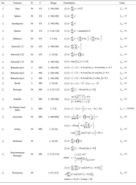
We have divided our experimental works into four sec- tions. In Section 4.1, we have done performance com- parison of WTLBO against basic algorithms like PSO, DE and TLBO to establish that our proposed approach performs better than above algorithms for investigated problems. We used 20 benchmark problems in order to test the performance of the PSO, DE, TLBO and the WTLBO algorithms. This set is large enough to include many different kinds of problems such as unimodal, mul- timodal, regular, irregular, separable, non-separable and multidimensional. For experiments in section 4.2 to Sec- tion 4.4 few functions from these 20 functions are used and those are mentioned in the comparison tables in re- spective sections of the paper. Initial range, formulation, characteristics and the dimensions of these problems are

listed in Table 1.

In Section 4.2 of our experiments, attempts are made to compare our proposed approach with the recent vari- ants of PSO as per [22,23]. The results of these variants are directly taken from [22,23] and compared with WT- LBO. In Section 4.3, the performance comparisons are made with the recent variants of DE as per [22]. The Sec- tion 4.4 of our experiments devote to the performance comparison of WTLBO with Artificial Bee Colony (ABC) variants as in [24-27]. Readers may be intimated here that in all such above mentioned comparisons we have simulated WTLBO and basic PSO, DE and TLBO of our own but gained results of other algorithms directly from the referred papers.

For comparing the speed of the algorithms, the first thing we require is a fair time measurement. The number of iterations or generations cannot be accepted as a time measure since the algorithms perform different amount of works in their inner loops, and they have different population sizes. Hence, we choose the number of fitness function evaluations (FEs)as a measure of computation

time instead of generations or iterations. Since the algo- rithms are stochastic in nature, the results of two succes- sive runs usually do not match. Hence, we have taken different independent runs (with different seeds of the random number generator) of each algorithm. Numbers of FEs for different algorithms which are compared with WTLBO are taken as in [22-27]. However, for WTLBO we have chosen 2.0 × 104 _{as maximum number of FEs.}

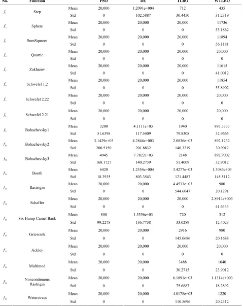
The exact numbers of FEs in which we get optimal re- sults with WTLBO are given in the Table 2.

Finally, we would like to point out that all the experi- ment codes are implemented in MATLAB. The experi- ments are conducted on a Pentium 4, 1 GB memory desktop in Windows XP 2002 environment

4.1. WTLBO vs PSO, DE and TLBO

In this Section, we have an exhaustive comparison of our proposed algorithm with various other evolutionary algo- rithms including basic TLBO. This section is divided into four sub sections, wherein we have compared WTLBO with various other algorithms. We have separately de- scribed the procedure in each sub section.

Parameter Settings

In all experiments in this section, the values of the com- mon parameters used in each algorithm such as popula- tion size and total evaluation number were chosen to be the same. Population size was 20 and the maximum num- ber fitness function evaluation was for all functions. The other specific parameters of algorithms are given below:

4

2.0 10

PSO Settings: Cognitive and social components, are

[image:4.595.60.535.100.744.2]

Table 1. List of benchmark functions have been used in experiment 1.

No. Function D C Range Formulation Value

1

f Step 30 US [−100,100]    2

1

0.5

D i i

f x x







 fmin0

2

f Sphere 30 US [−100,100]   2

1

D i i

f x x







fmin0

3

f SumSquares 30 US [−100,100]   2

1

D i i

f x i







x fmin0

4

f Quartic 30 US [−1.28,1.28]   4  

1

random 0,1

D i i

f x ix







 fmin0

5

f Zakharov 30 UN [−5,10]  

2 4

2

1 1 1

0.5 0.5

D D D

i i

i i i

i

f x x ix ix

                 







fmin0

6

f Schwefel 1.2 30 UN [−100,100]  

2 1 1

D i j i j

f x x

 

 

 _{ }

 

 

fmin0

7

f Schwefel 2.22 30 UN [−10,10]  

1 1

D D

i i i i

f x x

 









x fmin0

8

f Schwefel 2.21 30 [−100,100] f x max_i



xi,1 i D



fmin0

9

f Bohachevsky1 2 MS [−100,100]   2 2  

1 2 2 0.3cos 3π1 0.4cos(4π2) 0.7

f x x  x  x  x  fmin0

10

f Bohachevsky2 2 MS [−100,100]   2 2    

1 2 2 0.3cos 3π1 cos 4π2 0.3

f x x  x  x  x  fmin0

11

f Bohachevsky3 2 MS [−100,100]   2 2



   



1 2 2 0.3cos 3π1 4π2 0.3

f x x  x  x  x  fmin0 12

f Booth 2 MS [−10,10]     2 2

1 2 2 7 2 1 2 5

f x  x  x   x x  fmin0 13

f Rastrigin 30 MS [−5.12,5.12]   2  

1

10cos 2π 10

D

i i

i

f x x x



 





_   _ fmin0

14

f Schaffer 2 MN [−100,100]  













2 2 2 1 2 2 2 2 1 2 sin 0.5 1 0.001 x x f x x x   

  fmin0

15

f Six Hump Camel _Back 2 MN [−5,5]   2 4 6 2

1 1 1 1 2 2

1

2.1 4 4

3

4 2

f x x  x  x x x  x  x fmin 1.03163

16

f Griewank 30 MN [−600,600]   2

1 1

1 _{cos 1}

4000 D D i i i i x

f x x

i

 

 

  _{ }

 





fmin0

17

f Ackley 30 MN [−32,32]

    2 1 1 1

20 exp 0.2

1

exp cos 2 20

D i i D i i

f x x

D

pi x e

n       _ _      _   _   





min 0 f  18

f Multimod 30 [−10,10]  

1 1

D D

i i

i i

f x x

 







x fmin0

19

f Noncontinuous

Rastrigin 30 MS [−5.12,5.12]

  2  

1

10cos 2π 10

D

i i

i

f x y y







_   _

where _{ }

0.5 round 2 0.5 2 i i i _i i x x y _x x         min 0 f  20

f Weierstrass 30 [−0.5, 0.5]

 



 



 





max 1 0 max 0

cos 2 0.5

cos 2 0.5 ,

where 0.5, 3, max 20

D k k k i i k k k k i k

f x a b x

D a b x

a b k

      _{ }  _{ }  _      _  _   

 

[image:5.595.62.541.129.732.2]

Table 2. No. of fitness evaluation comparisons of PSO, DE, TLBO, WTLBO (mean and standard deviation over 30 inde- pendent runs) after each algorithm was terminated after running for 20,000 FEs or when it reached the global minimum value before completely running for 20,000 FEs.

No. Function PSO DE TLBO WTLBO

Mean 20,000 1.2091e+004 712 435

1

f Step

Std 0 102.5887 30.4450 31.2319

Mean 20,000 20,000 20,000 11736

2

f Sphere

Std 0 0 0 55.1862

Mean 20,000 20,000 20,000 11894

3

f SumSquares

Std 0 0 0 56.1181

Mean 20,000 20,000 20,000 20,000

4

f Quartic

Std 0 0 0 0

Mean 20,000 20,000 20,000 11615

5

f Zakharov

Std 0 0 0 41.0012

Mean 20,000 20,000 20,000 11854

6

f Schwefel 1.2

Std 0 0 0 55.8902

Mean 20,000 20,000 20,000 20,000

7

f Schwefel 2.22

Std 0 0 0 0

Mean 20,000 20,000 20,000 20,000

8

f Schwefel 2.21

Std 0 0 0 0

Mean 3200 4.1111e+03 1940 893.3333

9

f Bohachevsky1

Std 51.6398 117.5409 79.8308 32.9665

Mean 3.1429e+03 4.2844e+003 2.0836e+03 892.1232

10

f Bohachevsky2

Std 200.5150 201.8832 140.3219 30.9012

Mean 4945 7.7822e+03 2148 892.9002

11

f Bohachevsky3

Std 168.1727 140.2739 51.4009 32.9012

Mean 6420 1.2554e+004 3.4277e+03 1.3086e+03

12

f Booth

Std 18.3935 803.3543 121.4487 145.5112

Mean 20,000 20,000 4.4533e+03 980

13

f Rastrigin

Std 0 0 544.6047 20.1291

Mean 20,000 20,000 20,000 2.8914e+003

14

f Schaffer

Std 0 0 0 41.6333

Mean 800 1.5556e+03 720 312

15

f Six Hump Camel Back

Std 99.2278 136.7738 33.0289 12.4023

Mean 20,000 20,000 2916 980

16

f Griewank

Std 0 0 145.0686 20.1688

Mean 20,000 20,000 20,000 20,000

17

f Ackley

Std 0 0 0 0

Mean 20,000 20,000 3488 1040

18

f Multimod

Std 0 0 30.2715 23.9012

Mean 20,000 20,000 6.1891e+03 1.1314e+003

19

f Noncontinuous _Rastrigin

Std 0 0 75.6887 18.2892

Mean 20,000 20,000 4.0178e+03 1220

20

f Weierstrass

tween personal and population experience, respectively. In our experiments cognitive and social components were both set to 2. Inertia weight, which determines how the previous velocity of the particle influences the velocity in the next iteration, was 0.5.

DE Settings:In DE, F is a real constant which affects

the differential variation between two Solutions and set to F = 0.5 * (1 + rand (0,1)) where rand (0,1) is a uni-

formly distributed random number within the range [0,1] in our experiments. Value of crossover rate, which con- trols the change of the diversity of the population, was chosen to be R = (Rmax – Rmin) * (MAXIT–iter)/MAXIT

where Rmax = 1 and Rmin = 0.5 are the maximum and

minimum values of scale factor R, iter is the current it-

eration number and MAXIT is the maximum number of allowable iterations as recommended in [28].

TLBO Settings:For TLBO there is no such constant to

set.

WTLBO Settings: For WTLBO and are assigned as 0.9

and 0.1 respectively.

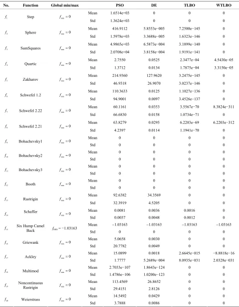
In Section 4.1, we compared the PSO, DE, TLBO and WTLBO algorithms on a large set of functions described in the previous section and are listed in Table 1. Each of the experiments in this section was repeated 30 times and it was terminated when it reached the maximum number of evaluations or when it reached the global minimum value with different random seeds and mean value and standard deviations of fitness value produced by the al- gorithms have been recorded in the Table 3 and at the same time mean value and standard deviations of No. of fitness evaluation produced by the algorithms have been recorded in the Table 2.

In order to analyze the results whether there is signifi- cance between the results of each algorithm, we per- formed t-test on pairs of algorithms which is quite popu-

lar among researchers in evolutionary computing [29]. In the Table 4 we report the statistical significance level of difference of the means of PSO and WTLBO algorithm, DE and WTLBO algorithm, TLBO and WTLBO algo- rithm. The t value is significant at a 0.05 level of signifi-

cance by two tailed test. In table “+” indicates the t value

is significant, and “NA” stands for Not applicable, cover- ing cases for which the two algorithms achieve the same accuracy results.

From the Table 4, we get that in 15 cases WTLBO is significant then PSO, where as in 14 cases WTLBO is significant than DE, in 8 cases WTLBO is significant than TLBO.

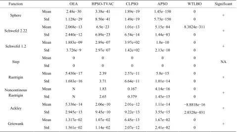
4.2. WTLBO vs OEA, HPSO-TVAC, CLPSO and APSO

The experiments in this section constitute the comparison of the WTLBO algorithm versus OEA, HPSO-TVAC,

CLPSO and APSO on 8 benchmarks described in [22],

where OEA uses the number of FEs and

HPSO-TVAC, CLPSO and APSO use the number of FEs, where as WTLBO runs for 2.0 × 104 _FEs.

The results of OEA, HPSO-TVAC, CLPSO and APSO are gained from [22] and [23] directly. In the last column of Table 5 shows the significance level between best and second best algorithm using t test at a 0.05 level of sig-

nificance by two tailed test. Note that here “+” indicates the t value is significant, and “NA” stands for Not appli-

cable, covering cases for which the two algorithms achi- eve the same accuracy results. As can be seen from Table 5, WTLBO greatly outperforms OEA, HPSO-TVAC, CL- PSO and APSO with better mean and standard deviation and numbers of FEs (refer Table 2 for WTLBO).

5

3.0 10

5

2.0 10

4.3. Experiment 3: WTLBO vs IADE, jDE and SaDE

The experiments in this section constitute the comparison of the WTLBO algorithm versus SaDE, jDE, JADE on 8 benchmark functions which are describe in [22]. The re- sults of JADE, jDE and SaDE are gained from [22] di- rectly. In the last column of Table 6 shows the signifi- cance level between best and second best algorithm using

t test at a 0.05 level of significance by two tailed test.

Note that here “+” indicates the t value is significant, and

“NA” stands for Not applicable, covering cases for which the two algorithms achieve the same accuracy results It can be seen from Table 6 that WTLBO performs much better than these DE variants on almost all the functions.

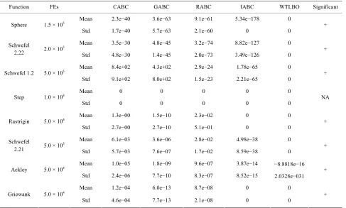
4.4. WTLBO vs CABC, GABC, RABC and IABC

The experiments in this section constitute the comparison of the WTLBO algorithm versus CABC [24], GABC [25], RABC [26] and IABC [27] on 8 benchmark func- tions. The parameters of the algorithms are identical to [26]. In the last column of Table 7 shows the signifi- cance level between best and second best algorithm using

t test at a 0.05 level of significance by two tailed test.

Note that here “+” indicates the t value is significant, and

“NA” stands for Not applicable, covering cases for which the two algorithms achieve the same accuracy results The results, which have been summarized in Table 7, show that WTLBO performs much better in most cases than these ABC variants.

5. Conclusion and Further Research

[image:7.595.59.536.121.733.2]

Table 3. Performance comparisons of PSO, DE, TLBO, WTLBO in term of fitness value (mean and standard deviation over 30 independent runs) after each algorithm was terminated after running for 20,000 FEs or when it reached the global mini- mum value before completely running for 20,000 FEs.

No. Function Global min/max PSO DE TLBO WTLBO

Mean 1.6514e+03 0 0 0

1

f Step fmin0

Std 1.3624e+03 0 0 0

Mean 416.9112 5.8553e−005 7.2500e−145 0

2

f Sphere fmin0

Std 1.5978e+03 3.3688e−005 1.6323e−146 0

Mean 4.9865e+03 6.5873e−004 3.1899e−140 0

3

f SumSquares fmin0

Std 2.0708e+04 3.8158e−004 1.9191e−141 0

Mean 2.7550 0.0525 2.3477e−04 4.5430e−05

4

f Quartic fmin0

Std 1.3712 0.0134 1.7875e−04 3.3150e−05

Mean 214.9360 127.9620 3.2475e−145 0

5

f Zakharov fmin0

Std 46.9318 26.9070 3.0237e−146 0

Mean 110.3633 0.0125 1.1027e−136 0

6

f Schwefel 1.2 fmin0

Std 94.9001 0.0097 3.4526e−137 0

Mean 60.1161 0.0353 3.5567e−70 8.3824e−311

7

f Schwefel 2.22 fmin0

Std 66.6830 0.0158 1.0734e−71 0

Mean 63.8279 0.0295 6.2203e−69 6.2203e−312

8

f Schwefel 2.21 fmin0

Std 4.2397 0.0114 1.1941e−70 0

Mean 0 0 0 0

9

f Bohachevsky1 fmin0

Std 0 0 0 0

Mean 0 0 0 0

10

f Bohachevsky2 fmin0

Std 0 0 0 0

Mean 0 0 0 0

11

f Bohachevsky3 fmin0

Std 0 0 0 0

Mean 0 0 0 0

12

f Booth fmin0

Std 0 0 0 0

Mean 92.6382 34.3569 0 0

13

f Rastrigin fmin0

Std 32.3919 4.5205 0 0

Mean 0.0081 0.0036 0.0016 0

14

f Schaffer fmin0

Std 0.0037 0.0048 0.0012 0

Mean 1.03163 1.03163 1.03163 1.03163

15

f Six Hump Camel _Back fmin = −1.03163

Std 0 0 0 0

Mean 5.0658 0.0030 0 0

16

f Griewank fmin0

Std 20.7782 0.0049 0 0

Mean 15.0899 0.0018 2.6645e−015 −8.8818e−16

17

f Ackley fmin0

Std 1.7777 5.2689e−004 8.0935e−031 2.0328e−031

Mean 2.7033e−107 1.8643e−124 0 0

18

f Multimod fmin0

Std 1.4786e−106 1.0200e−123 0 0

Mean 113.4569 26.8652 0 0

19

f Noncontinuous _Rastrigin fmin0

Std 29.4151 2.8126 0 0

Mean 14.5492 0.0429 0 0

20

f Weierstrass fmin0

[image:8.595.54.538.102.420.2]

Table 4. t value, significant at a 0.05 level of significance by two tailed test using Table 3.

Function No. PSO/WTLBO DE/WTLBO TLBO/WTLBO

1

f + NA NA

2

f + + +

3

f + + +

4

f + + +

5

f + + +

6

f + + +

7

f + + +

8

f + + +

9

f NA NA NA

10

f NA NA NA

11

f NA NA NA

12

f NA NA NA

13

f + + NA

14

f + + +

15

f NA NA NA

16

f + + NA

17

f + + NA

18

f + + NA

19

f + + NA

20

f + + NA

Table 5. Performance comparisons WTLBO, OEA, HPSO-TVAC, CLPSO and APSO in term of fitness value (mean and standard deviation over 30 independent runs) after OEA running of 3.0 × 105 FEs, HPSO-TVAC, CLPSO and APSO use running 2.0 × 105 FEs, and WTLBO running for 2.0 × 104_.

Function OEA HPSO-TVAC CLPSO APSO WTLBO Significant

Mean 2.48e−30 3.38e−41 1.89e−19 1.45e−150 0

Sphere

Std 1.128e−29 8.50e−41 1.49e−19 5.73e−150 0 +

Mean 2.068e−13 6.9e−23 1.01e−13 5.15e−84 8.3824e−311

Schwefel 2.22

Std 2.440e−12 6.89e−23 6.54e−14 1.44e−83 0 +

Mean 1.883e−09 2.89e−07 3.97e+02 1.0e−10 0

Schwefel 1.2

Std 3.726e−9 2.97e−07 1.42e+02 2.13e−10 0 +

Mean 0 0 0 0 0

Step

Std 0 0 0 0 0 NA

Mean 5.430e−17 2.39 2.57e−11 5.8e−15 0

Rastrigin

Std 1.683e−16 3.71 6.64e−11 1.01e−14 0 +

Mean N 1.83 0.167 4.14e−16 0

Noncontinous

Rastrigin _{Std N 2.65 0.379 1.45e−15 0} +

Mean 5.336e−14 2.06e−10 2.01e−12 1.11e−14 −8.8818e−16

Ackley

Std 2.945e−13 9.45e−10 9.22e−13 3.55e−15 2.0328e−031 +

Mean 1.317e−02 1.07e−02 6.45e−13 1.67e−02 0

Griewank

[image:8.595.61.540.465.731.2]

[image:9.595.57.545.110.408.2]

Table 6. Performance comparisons WTLBO, IADE, jDE and SaDE in term of fitness value (mean and standard deviation over 30 independent runs) after each algorithm was terminated after running by given FEs.

Function FEs SaDE jDE JADE WTLBO Significant

Mean 4.5e−20 2.5e−28 1.8e−60 0

Sphere 1.5 × 105

Std 1.9e−14 3.5e−28 8.4e−60 0

+

Mean 1.9e−14 1.5e−23 1.8e−25 0

Schwefel 2.22 2.0 × 105

Std 1.1e−14 1.0e−23 8.8e−25 0 +

Mean 9.0e−37 5.2e−14 5.7e−61 0

Schwefel 1.2 5.0 × 105

Std 5.4e−36 1.1e−13 2.7e−60 0

+

Mean 9.3e+02 1.0e+03 2.9e+00 0

Step 1.0 × 104

Std 1.8e+02 2.2e+02 1.2e+00 0 +

Mean 1.2e−03 1.5e−04 1.0e−04 0

Rastrigin 1.0 × 105

Std 6.5e−04 2.0e−04 6.0e−05 0 +

Mean 7.4e−11 1.4e−15 8.2e−24 0

Schwefel 2.21 5.0 × 105

Std 1.82e−10 1.0e−15 4.0e−23 0 +

Mean 2.7e−03 3.5e−04 8.2e−10 −8.8818e−16

Ackley 5.0 × 104

Std 5.1e−04 1.0e−04 6.9e−10 2.0328e−031

+

Mean 7.8e−04 1.9e−05 9.9e−08 0

Griewank

5.0 × 104

Std 1.2e−03 5.8e−05 6.0e−07 0 +

Table 7. Performance comparisons of WTLBO, CABC, GABC, RABC and IABC in term of fitness value (mean and standard deviation over 30 independent runs) after each algorithm was terminated after running by given FEs.

Function FEs CABC GABC RABC IABC WTLBO Significant

Mean 2.3e−40 3.6e−63 9.1e−61 5.34e−178 0

Sphere 1.5 × 105

Std 1.7e−40 5.7e−63 2.1e−60 0 0 +

Mean 3.5e−30 4.8e−45 3.2e−74 8.82e−127 0

Schwefel

2.22 2.0 × 10

5

Std 4.8e−30 1.4e−45 2.0e−73 3.49e−126 0 +

Mean 8.4e+02 4.3e+02 2.9e−24 1.78e−65 0

Schwefel 1.2 5.0 × 105

Std 9.1e+02 8.0e+02 1.5e−23 2.21e−65 0 +

Mean 0 0 0 0 0

Step 1.0 × 104

Std 0 0 0 0 0 NA

Mean 1.3e−00 1.5e−10 2.3e−02 0 0

Rastrigin 5.0 × 104

Std 2.7e−00 2.7e−10 5.1e−01 0 0 +

Mean 6.1e−03 3.6e−06 2.8e−02 4.98e−38 0

Schwefel

2.21 5.0 × 10

5

Std 5.7e−03 7.6e−07 1.7e−02 8.59e−38 0 +

Mean 1.0e−05 1.8e−09 9.6e−07 3.87e−14 −8.8818e−16

Ackley 5.0 × 104

Std 2.4e−06 7.7e−10 8.3e−07 8.52e−15 2.0328e−031

+

Mean 1.2e−04 6.0e−13 8.7e−08 0 0

Griewank 5.0 × 104

[image:9.595.57.544.443.736.2]

ques like PSO, DE, ABC and its variants. The proposed approach, known as Weighted-TLBO (WTLBO) is based on the natural phenomena of human brain (a learner’s brain) in forgetting the lessons learnt in last session. The paper suggested an inclusion of a parameter known as “weight” to address this phenomenon while using the learning equation in teaching and learning phases of ba- sic TLBO algorithm. Although, inclusion of a parameter such as weight might seem to increase the complexity of the basic TLBO algorithm while tuning the parameter, the suggested approach in our work in setting up the weight parameter eases the task and able to provide bet- ter results compared to basic TLBO and all other inves- tigated algorithms in this work for several benchmark functions. Our proposed WTLBO not only able to find global optima results but also does in faster computation time. This fact is verified from the number of function evaluations for WTLBO in each case from the results shown in our paper.

As a further research, we need to verify how this ap- proach behaves with many other benchmark functions and some real world problems in data clustering.

REFERENCES

[1] R. V. Rao, V. J. Savsani and D. P. Vakharia, “Teaching- Learning-Based Optimization: A Novel Method for Con- strained Mechanical Design Optimization Problems,” Computer-Aided Design, Vol. 43, No. 1, 2011, pp. 303- 315. doi:10.1016/j.cad.2010.12.015

[2] R. V. Rao, V. J. Savsani and D. P. Vakharia, “Teach- ing-Learning-Based Optimization: An Optimization Me- thod for Continuous Non-Linear Large Scale Problems,” INS 9211 No. of Pages 15, Model 3G 26 August 2011. [3] R. V. Rao, V. J. Savsani and J. Balic, “Teaching Learning

Based Optimization Algorithm for Constrained and Un- constrained Real Parameter Optimization Problems,” En- gineering Optimization, Vol. 44, No. 12, 2012, pp. 1447- 1462. doi:10.1080/0305215X.2011.652103

[4] R. V. Rao and V. K. Patel, “Multi-Objective Optimization of Combined Brayton and Inverse Brayton Cycles Using Advanced Optimization Algorithms,” Engineering Opti- mization, Vol. 44, No. 8, 2012, pp. 965-983.

doi:10.1080/0305215X.2011.624183

[5] R. V. Rao and V. J. Savsani, “Mechanical Design Opti- mization Using Advanced Optimization Techniques,” Springer-Verlag, London, 2012.

doi:10.1007/978-1-4471-2748-2

[6] V. Toğan, “Design of Planar Steel Frames Using Teach- ing-Learning Based Optimization,” Engineering Struc- tures, Vol. 34, 2012, pp. 225-232.

doi:10.1016/j.engstruct.2011.08.035

[7] R. V. Rao and V. D. Kalyankar, “Parameter Optimization of Machining Processes Using a New Optimization Algo- rithm,” Materials and Manufacturing Processes, Vol. 27, No. 9, 2011, pp. 978-985.

doi:10.1080/10426914.2011.602792

[8] S. C. Satapathy and A. Naik, “Data Clustering Based on Teaching-Learning-Based Optimization. Swarm, Evolu- tionary, and Memetic Computing,” Lecture Notes in Com- puter Science, Vol. 7077, 2011, pp. 148-156,

doi:10.1007/978-3-642-27242-4_18

[9] J. H. Holland, “Adaptation in Natural and Artificial Sys- tems,” University of Michigan Press, Ann Arbor, 1975. [10] J. G. Digalakis and K. G. Margaritis, “An Experimental

Study of Benchmarking Functions for Genetic Algori- thms,” International Journal of Computer Mathematics, Vol. 79, No. 4, 2002, pp. 403-416.

doi:10.1080/00207160210939

[11] R. C. Eberhart and Y. Shi, “Particle Swarm Optimization: Developments, Applications and Resources,” IEEEPro- ceedings of International Conference on Evolutionary Computation, Vol. 1, 2001, pp. 81-86.

[12] R. C. Eberhart and Y. Shi, “Comparing Inertia Weights and Constriction Factors in Particle Swarm Optimiza- tion,” IEEE Proceedings of International Congress on Evolutionary Computation, Vol. 1, 2000, pp. 84-88. [13] J. Kennedy and R. Eberhart, “Particle Swarm Optimiza-

tion,” IEEE Proceedings of International Conference on Neural Networks, Vol. 4, 1995, pp. 1942-1948.

doi:10.1109/ICNN.1995.488968

[14] J. Kennedy, “Stereotyping: Improving Particle Swarm Performance with Cluster Analysis,” IEEE Proceedings of International Congress on Evolutionary Computation, Vol. 2, 2000, pp. 303-308.

[15] Y. Shi and R. C. Eberhart, “Comparison between Genetic Algorithm and Particle Swarm Optimization,” Lecture Notes in Computer Science—Evolutionary Programming VII, Vol. 1447, 1998, pp. 611-616.

[16] Y. Shi and R. C. Eberhart, “Parameter Selection in Par- ticle Swarm Optimization,” Lecture Notes in Computer Science Evolutionary Programming VII, Vol. 1447, 1998, pp. 591-600. doi:10.1007/BFb0040810

[17] Y. Shi and R. C. Eberhart, “Empirical Study of Particle Swarm Optimization,” IEEEProceedings of International Conference on Evolutionary Computation, Vol. 3, 1999, pp. 101-106.

[18] R. Storn and K. Price, “Differential Evolution—A Simple and Efficient Heuristic for Global Optimization over Con- tinuous Spaces,” Journal of Global Optimization, Vol. 11, No. 4, 1997, pp. 341-359. doi:10.1023/A:1008202821328 [19] R. Storn and K. Price, “Differential Evolution—A Simple

and Efficient Adaptive Scheme for Global Optimization over Continuous Spaces,” Technical Report, International Computer Science Institute, Berkley, 1995.

[20] K. Price, R. Storn and A. Lampinen, “Differential Evolu-tion a Practical Approach to Global OptimizaEvolu-tion,” Sprin- ger Natural Computing Series, Springer, Heidelberg, 2005.

[21] S. Das, A. Konar and U. K. Chakraborty, “Two Improved Differential Evolution Schemes for Faster Global Search,” Genetic and Evolutionary Computation Conference, Wa- shington DC, 25-29June 2005.

tems, Man, and Cybernetics—Part B, Vol. 39, No. 6, 2009, pp. 1362-1381. doi:10.1109/TSMCB.2009.2015956 [23] A. Ratnaweera, S. Halgamuge and H. Watson, “Self-Or-

ganizing Hierarchical Particle Swarm Optimizer with Time-Varying Acceleration Coefficients,” IEEE Transac- tions on Evolutionary Computation, Vol. 8, No. 3, 2004, pp. 240- 255. doi:10.1109/TEVC.2004.826071

[24] B. Alatas, “Chaotic Bee Colony Algorithms for Global Numerical Optimization,” Expert Systems with Applica- tions, Vol. 37, No. 8, 2010, pp. 5682-5687.

doi:10.1016/j.eswa.2010.02.042

[25] G. P. Zhu and S. Kwong, “Gbest-Guided Artificial Bee Colony Algorithm for Numerical Function Optimization,” Applied Mathematics and Computation, Vol. 217, No. 7, 2010, pp. 3166-3173. doi:10.1016/j.amc.2010.08.049 [26] F. Kang, J. J. Li and Z. Y. Ma, “Rosenbrock Artificial

Bee Colony Algorithm for Accurate Global Optimization

of Numerical Functions,” Information Sciences, Vol. 181, No. 16, 2011, pp. 3508-3531.

doi:10.1016/j.ins.2011.04.024

[27] W. F. Gao and S. Y. Liu, “Improved Artificial Bee Col- ony Algorithm for Global Optimization,” Information Processing Letters, Vol. 111, No. 17, 2011, pp. 871-882.

doi:10.1016/j.ipl.2011.06.002

[28] S. Das and A. Abraham and A. Konar, “Automatic Clus- tering Using an Improved Differential Evolution Algo- rithm,” IEEE Transactions on Systems, Man, and Cyber- netics—Part A: Systems and Humans, Vol. 38, No. 1, 2008.

[29] S. Das, A. Abraham, U. K. Chakraborty and A. Konar, “Differential Evolution Using a Neighborhood-Based Mu- tation Operator,” IEEE Transactions on Evolutionary Computation, Vol. 13, No. 3, 2009, pp. 526-553.