Attention Guided Organized Perception and Learning of Object Categories Based on Probabilistic Latent Variable Models

(1)

Attention-Guided Organized Perception and Learning of

Object Categories Based on Probabilistic Latent

Variable Models

Masayasu Atsumi

Department of Information Systems Science, Faculty of Engineering, Soka University, Tokyo, Japan. Email: [email protected]

Received November 16th_,_{2012; revised April 19}th_{, 2013; accepted April 26}th_{, 2013}

Copyright © 2013 Masayasu Atsumi. This is an open access article distributed under the Creative Commons Attribution License, which permits unrestricted use, distribution, and reproduction in any medium, provided the original work is properly cited.

ABSTRACT

This paper proposes a probabilistic model of object category learning in conjunction with attention-guided organized perception. This model consists of a model of attention-guided organized perception of object segments on Markov random fields and a model of learning object categories based on a probabilistic latent component analysis. In attention- guided organized perception, concurrent figure-ground segmentation is performed on dynamically-formed Markov random fields around salient preattentive points and co-occurring segments are grouped in the neighborhood of selective attended segments. In object category learning, a set of classes of each object category is obtained based on the probabilistic latent component analysis with the variable number of classes from bags of features of segments extracted from images which contain the categorical objects in context and an object category is represented by a composite of object classes. Through experiments using two image data sets, it is shown that the model learns a probabilistic structure of intra-categorical composition and inter-categorical difference of object categories and achieves high performance in object category recognition.

Keywords: Attention; Perceptual Organization; Probabilistic Learning; Object Categorization

1. Introduction

Human visual processing is guided through attention which circumscribes regions for high-level processing such as learning and recognition. An attention process can be divided into two stages of a preattentive process and a focal attentional process [1]. In the preattentive process, local saliency is detected in parallel over the entire visual field. In the focal attentional process, they are successively integrated and attention works in two distinct and complementary modes of a space-based mode and an object-based mode [2], in which the former selects locations where finer segmentation is promoted and the latter selects organized segments of objects through figure-ground segmentation and perceptual organization, and they operates in concert to influence the allocation of attention. Organized percept of segments tends to attract attention automatically [3]. Thus attention and organized perception can affect the high-level processing of learning and recognition.

The problem to be addressed in this paper is learning

(2)

of selective attended segments. In learning object categories, a set of object classes which composes each object category is obtained based on the PLCA with the variable number of classes (V-PLCA) from bags of features (BoFs) [7] of segments extracted from images in the object category. Here a BoF of a segment is calculated by using a code book which is a set of key features gener- ated by clustering SIFT features [8] of salient points of all the segments extracted from a set of all the scene images. The V-PLCA learns a probabilistic structure of object classes in each object category where an object class represents an appearance of the categorical object or another co-occurring categorical object and a composite of object classes represents an object category.

As for related work, there have been proposed a lot of computational models of visual attention, in which a saliency map model [9] is well-known and have a great influence on later studies [10-14]. Image segmentation methods based on MRF models, which date back to Ge- man’s work [15], are also widely studied and there has been proposed an attention-based segmentation method using MRF [16]. There has also been proposed a salient object detection method using a conditional random field [17]. Our model of attention-guided organized perception is unique as it links spatial preattention and object-based attention through figure-ground segmentation on dynamically-formed MRFs and groups segments in the neighborhood of selective attended segments. There have been proposed several methods which apply probabilistic latent semantic analysis to learning object or scene categories [18-20] and incorporate attention into object recognition [21]. It is known that context improves category recognition of ambiguous objects in a scene [22] and there have been proposed several methods which incur- porate context into object categorization [23-28]. The difference of our learning method from those existing ones is that it uses attended co-occurring segments for learning and it learns a probabilistic structure of each

categorical object and its context which make it possible to recognize objects in context.

This paper is organized as follows. Section 2 presents a model of attention-guided organized perception. Sec- tion 3 describes a probabilistic learning model of object categories. Experimental results are shown in Section 4 in which the Caltech-256 image data set is used for evaluating learning through attention-guided organized perception and the MSRC labeled image data set v2 is used for evaluating recognition through categorical ob-ject learning. We discuss our results in Section 5 and conclude our work in Section 6.

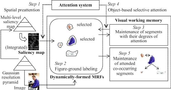
2. Attention-Guided Organized Perception

The model of attention-guided organized perception consists of a saliency map for preattention, a collection of dynamically-formed MRFs for figure-ground segmentation, a visual working memory for maintaining segments and perceptually organizing them around selective attention, and an attention system on a saliency map and a visual working memory. Figure 1 depicts the organiza-

tion and the computational steps of the model, which are explained in the following subsections.

2.1. Saliency Map

[image:2.595.153.442.564.717.2]

A saliency map is in general computed by integrating several visual features such as contrast, orientation, mo- tion and so forth. A saliency map in this paper is a sim- plified model of a multi-level saliency map which is proposed in [12]. As features of an image, brightness, hue and their contrast are obtained on a Gaussian resolution pyramid of the image. Brightness contrast and hue contrast are respectively computed by convolving brightness and hue with a LoG (Laplacian of a Gaussian) ker- nel. However, since a hue value represents a color category by an angle in



0, 2π



on a continuous color spec- trum circle, hue contrast is obtained by performing con-

(3)

volution for hue difference of each point with its neighboring points. A saliency map is obtained by calculating saliency from brightness contrast and hue contrast on each level of a Gaussian resolution pyramid [12] and combining the multi-level saliency into one map by tak- ing a sum of them.

[image:3.595.339.538.347.413.2]

2.2. Segmentation through Preattention

Figure-ground segmentation is performed by figure- ground labeling on dynamically-formed MRFs of brightness and hue around preattentive points. In the first step (Figure 1), plural preattentive points are stochastically

selected from a saliency map according to their degrees of saliency. In the second step (Figure 1), initial 2-di-

mensional MRFs of brightness and hue are dynamically allocated around the preattentive points and figure- ground labeling is iterated by gradually expanding the MRFs by a certain margin until figure segments converge or the specified number of iterations is reached. If plural figure segments satisfy a mergence condition, they are merged into one segment.

The figure-ground labeling on a MRF is formulated as

follows. Let be a set of segment labels

where “1” represents a figure label and “−1” represents a

ground label and let be an observation of

features where b is brightness and h is hue. Let W be a domain of a MRF and let



1, 1

L 

z







b h,





w , w

l l w W l L



be

segment labels on W. Then, for a given observed feature

w W, the problem of estimating segment labels is

solved by using the EM algorithm with the mean field approximation [29]. The mean field local energy function using mean field approximation is defined by

 

w

z z _

 



_, t



_log



_,  t



_{ }

mf mf

w w w w w

U l z    p z l  U l (1)

and

 



,





8

w w

mf

w w w w

w B w B

U l V l l   l , l_w



 





 



 (2)

where V is potential of a pair-site clique, Bw is the 8-

neighborhood system,  is an interaction coefficient which is preset in this study, lw is an expectation of a

segment label in the neighborhood, t is the EM iteration number and is a parameter set that determines distributions of





,



p z l  . Concretely, is means and

variances of multivariate Gaussian distributions of figure and ground features. Then, a posterior probability of a segment label is given by



 



,



exp



,  



t mf

w w t

mf

w w mf

w

U l

p l

H

 

  z

z _ (3)

where mf w

H is the partition function and an expectation

of a segment label is obtained as

 







,



w t mf

w w w w w

l L

l l p l







 

z z . (4)

In the E-step, for each point in a domain of a MRF, an expectation of the segment label l zw w is repeatedly

calculated until all the expectations of segment labels converge. Usually, only a few iterations are required to converge. A segment label is estimated as “1” if

0

w w

l z  and “−1” otherwise. In the M-step, means

and variances of multivariate Gaussian distributions for figure and ground features are updated by using results of the E-step.

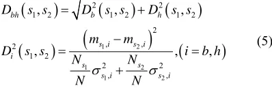
The mergence of segments is performed if they spa- tially overlap and the Mahalanobis generalized distance for brightness and hue between them is not greater than a certain threshold. Let s₁ and s₂ be a pair of segments.

Then the Mahalanobis generalized distance Dbh



s s₁, ₂



for brightness and hue between s₁ and s₂ is defined

by



















1 2





1 2

2 2

1 2 1 2 1 2

2 , , 2 1 2 2 2 , , , , , , ,

bh b h

s i s i i

s s

s i s i

D s s D s s D s s

m m

D s s i b h

N N

N  N 

 



 





, (5)

where, for s



s s₁, ₂



, m_{s b}_, and ms h, 2 ,

are means of brightness and hue respectively and _{s b} and 2

,

s h

 are

variances of brightness and hue respectively. The N_s₁ and N_s₂ are the number of points of s1 and s2 where

1 2

s Ns

NN  .

2.3. Organized Perception through Object-Based Attention

Figure segments are maintained in a visual working memory and organized perception is performed around selective attended segments through object-based attention. In the third step (Figure 1), for each extracted fig-

(4)

whether or not it extends outside the bounds of an image. A segment is defined as closed if it does not intersect with the border of an image at more than a specified number of points. Attention bias represents a priori or experientially acquired attentional tendency to a region with a particular feature such as a face-like region. In experiments in Section 4, a segment is judged as a face by simply using its hue and aspect ratio. Then, the attention degree A s

 

of a segment s is defined by

 

,



s s

 

p p

 

b b

 



A s  s   A s  A s  A s

(6) where A ss

 

is the degree of surface attention, Ap

 

s

is the degree of spot attention, A sb

 

1, 0 is the attention

bias, and s p b s p b are weighting

coefficients for them respectively. The function



, ,

     



 

s,

 

takes 1 if a segment s is closed and  otherwise, where is the decrease rate of attention when the segment isn’t closed.



0 1

  



In the fourth step (Figure 1), from these segments, the

specified number of segments whose attention degree are larger than others are selected as selective attended segments. In the fifth step (Figure 1), each selective at-

tended segment and its neighboring segments are grouped as a co-occurring segment. If two sets of co-occurring segments overlap, they are combined into one co-occurring segment. This makes it possible to group part segments of an object or group salient contextual segments with an object.

3. Probabilistic Learning of Object

 

c i,j hc i,j

 

f1 , ,hc i,j

 

fNF

H s    _

of each segment sc i,j is calculated for SIFT features of

its salient points by using this code book.

3.2. Learning about Object Categories

The V-PLCA computes a probabilistic structure of classes



, r 1,,



c c

Q  q  N

c

r Q for each category cC where

,

c r is a r-th class of a category c and Qc is the num-

ber of classes in c. Here the problem to be solved is

estimating probabilities

q N

Q



,



 

qc r,



, qc r



p





 

, ,

j j

c i c i n c r

r

p s f_n 



p p s f q

namely class probabilities





condi-

tional probabilities of segments , ,

,

c r c r c

p q q Q







p sc i,j qc r, sc i,jS qc, c r, Qc



,

conditional probability distributions of key features







p f qn c r, fnF q, c r, Qc



,



,j fn

and the number of classes that maximize the following log-likelihood Qc

N

 



,j log , j

c c i n c i

i n

L 



h f p s (7)

for a set of BoFs



 

_, _,



.

j j

c c i c i c

H  H s s S The class

probability represents the composition ratio of object classes in an object category, the conditional probability of segments represents the degree to which object segments are instances of an object class and the conditional probability distribution of key features represents the feature of an object class.

(5)

[E-step]





 









 









, , , , , , , , , , , j j j

c r c i c r n c r c r c i n

c r c i c r n c r r

p q p s q p f q

p q s f

p q p s q p f q

                 



 (8) [M-step]





 





 





, , , , , , , , , j j j j j j

c i n c r c i n i

n c r

c i n c r c i n n i

h f p q s f

p f q

h f_ p q s f

 



 

 (9)





,

 

_{ }



_

, ,



_

, , , , , , , j j j j j j

c i n c r c i n n

c i c r

c i n c r c i n i n

h f p q s f

p s q

h  f p q s  f







 

(10)

 

,

 



_{ }

, ,



, , , j j j j

c i n c r c i n

i n

c r

c i n i n

h f p q s f

p q h f 

 

j (11)

where  is a temperature coefficient.

The number of classes is determined through an EM iterative process with subsequent class division. The process starts with one or a few classes, pauses at every certain number of EM iterations less than an upper limit and calculates the following index, which is called the dispersion index,













, , , , , ,

c r j j

j

q n c r c i n c i

i n

p f q d s f p s q

  __  _ _

 

 

c r

(12) where





,

 

_{ }

, , , j j j c i n c i n

c i n n

h f

d s f

h f_







(13) for c r, c. Then a class whose dispersion index

takes the maximum value among all classes is divided into two classes. This iterative process is continued until

,

c r

q

q Q

 

 -values for all classes become less than a certain threshold. The class is divided into two classes as follows. Let be a source class to be divided and let c r,₁ and c r,0 be target classes after division. Then, for a

q 2 , c r q q

segment sc i,_jarg maxi_j



p s



c i,_j qc r,₀





F

 

which has the

maximum conditional probability and its BoF

 

c i,j c i,j

 

1 , , c i,j

 

N

H s _  h _ f  h _ f ,

one class c r,₁ is set by specifying its conditional probability distribution of key features, conditional probabilities of segments and a class probability as

q



1



_

 

_{ }

_

, , , * , j j

c i n

n c r n

c i n n

h f

p f q f F

h f        





c i,j c r,1

 

c i,j c r,0



, c i, c

p s q p s q s S

j

   (15)

   

0

1 , , 2 c r c r p q

p q  (16)

respectively where  is a positive correction coefficient. Another class c r,₂ is set by specifying its conditional probability distribution of key features

q







p f qn c r,2 fnF



at random, conditional probabilities of segments



p s



c i,_j qc r,₂



sc i,_jSc



as 0 for sc i,_j

and 1





c S

N 1 for other segments, and a class prob-

ability as

 

c r,₂

 

c r,₀ . As a result of subse-

quent class division, classes can be represented in a binary tree form.

2

p q  p q

The temperature coefficient  is set to 1.0 until the number of classes is fixed and after that it is gradually decreased according to a given schedule of the tempered EM until convergence.

The feature of an object category is represented by composing conditional probability distributions of key features of classes in the category. A composite probability distribution of key features for an object category c is obtained for a set of classes Qc



qc r, qc r, Qc



as







  



,

c r c

n c c r n c r

q Q

p f Q p q p f q







 _, . (17)

4. Experiments

Two experiments were conducted to evaluate attention- guided organized perception and learning of object categories. The first experiment evaluates learning through attention-guided organized perception by using the Cal- tech-256 image data set [31] and the second experiment evaluates recognition through learning about object categories by using the MSRC labeled image data set v21_.

4.1. Experiment of Learning through

Attention-Guided Organized Perception

The Caltech-256 image data set was used for evaluating learning through attention-guided organized perception. For each of 20 categories, 4 images, each of which contains the categorical object and other categorical objects in context, were selected and used for experiments. Fig- ure 2 shows some categorical images.

  (14)

Main parameters were set as follows. The number of levels of a Gaussian resolution pyramid was 5. As for attention-guided organized perception, an interaction coefficient  was 1.5, a threshold for segment mergence

(6)

[image:6.595.58.287.95.246.2]

Figure 2. Examples of images. Images of 20 categories (“bear”, “butterfly”, “chimp”, “dog”, “elk”, “frog”, “gi- raffe”, “goldfish”, “grasshopper”, “helicopter”, “hibiscus”, “horse”, “hummingbird”, “ipod”, “iris”, “palm-tree”, “people”, “school-bus”, “skyscraper” and “telephone-box”) were used in experiments.

was 1.0, weighting coefficients and a decrease rate for the attention degree of segments in the expression (6) were _s0.5,_p0.5,_b1.0 and  0.2 respectively, and the upper bound number of selective attention was 4. As for learning, a threshold for salient points was 0.1, a threshold of class division was 0.07 and a correction coefficient in the expression (14) was 2.0. In the tempered EM, a temperature coefficient  was decreased by multiplying it by 0.95 at every 20 iterations until it became 0.8.

[image:6.595.308.535.188.362.2]

Learning was performed for a set of co-occurring segments extracted from images of each category through the attention-guided organized perception. The number of salient points, that is, 128-dimensional SIFT features which were extracted from all these segments was 76019. The code book size of key features which were obtained by the K-tree method was 438. The BoFs were calculated for 181 segments whose numbers of salient points were more than 100.

Figure 3 shows co-occurring segments and their labels

for some categorical images which were extracted by the attention-guided organized perception. There were observed three types of co-occurring segments. The first type of co-occurring segments represents organized perception in which an object consists of one segment and it is grouped with its contextual segments. Examples of “telephone-box” and “hibiscus” in Figure 3 show organ-

ized perception of this type. The second type of co-occurring segments represents organized perception in which each co-occurring segment is a part of an object and the object consists of those segments. Examples of “people” and “school-bus” in Figure 3 show organized

perception of this type. The third type of co-occurring segments represents organized perception in which an

object consists of plural segments and it is also grouped with its contextual segments. Examples of “chimp” and “butterfly” in Figure 3 show organized perception of this

type.

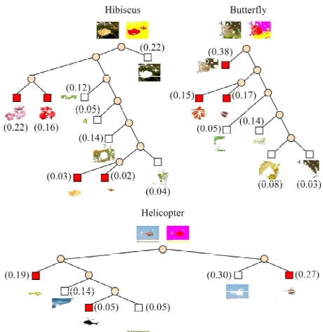
Figure 4 shows some results of the V-PLCA, that is,

[image:6.595.308.538.407.643.2]

object classes for some object categories in a binary tree form. In Figure 4, a typical segment of a class r of each

Figure 3. Examples of (a) images, (b) co-occurring segments and (c) labels for some categories. Different labels are illus- trated by different colors.

(7)

category c is a segment sc i,_j that maximizes p q



c r, sc i,j



.

The mean number of classes per a category was 7.55.

4.2. Experiment of Recognition through Learning about Object Categories A composite probability distribution of key features

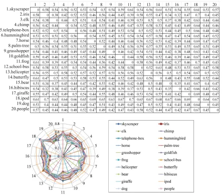
for an object category is a weighted sum of conditional probability distributions of key features for its object classes with their class probabilities. Figure 5 shows

composite probability distributions of key features for all categories and Figure 6 shows distance between each

pair of them which is defined by the following expression

The MSRC labeled image data set v2 was used for evaluating recognition through learning about object categories. This data set contains 23 object categories and each image has a pixel level ground truth in which each pixel is labeled as one of 23 object categories or “void”. Most images are associated with more than one object category. A collection of 14 sets of images each set of which con- tained about 30 images and each image in it had the same categorical object that was considered to be in the fore- ground and other categorical objects in the background were arranged from this data set. This made 14 object categories and an image in each object category con- tained an object with the category label and other co- occurring objects with other labels in 23 category labels. The total number of images was 420. Figure 7 shows

some categorical images and their object segments with labels. In this experiment, labeled co-occurring object







1

 



1 2 1 ,

2

n c n c

n c c

p f Q p f Q

L Q Q







2

(18)

for any different categories c₁ and c2. Each category

had a different probability distribution of key features and the mean distance of all pairs of categories was 0.51. These make it possible to distinguish each object category from others by their composite probability distributions of key features.

[image:7.595.60.539.342.721.2]

Q Q

(8)

[image:8.595.79.522.94.484.2]

Figure 6. Distance between probability distributions of key features for pairs of object categories.

Figure 7. Examples of (a) categorical images, (b) color-labeled images and (c) co-occurring segments with labels. Images of 14 categories (“tree”, “building”, “airplane”, “cow”, “person”, “car”, “bicycle”, “sheep”, “sign”, “bird”, “chair”, “cat”, “dog”,

boat”) were used in experiments. Here a face and a body were interpreted as a person. “

[image:8.595.157.441.510.698.2]

(9)

segments are supposed to be extracted from an image by attention-guided organized perception and used for learning and recognition. Images in object categories were split into two parts for 2-fold cross validation. In order to represent features of segments, 128-dimensional SIFT features of keypoints in all the segments were clustered by the K-tree method to generate a set of key features as a code book and a BoF of each segment was calculated for its 128-dimensional SIFT features at keypoints by using this code book. The code book sizes of key features were 412 and 438 for two learning sets respectively.





 

_{ }

arg min i n n c

c C n n n

h f

c p f Q

h f



 _ _









(19) where cis a recognized object category and

 

i

 

1 , , i

 

NF

H i  h f  h f _ is a BoF for an input cate-

gorical image i. Table 1 shows the average classification

accuracy of two image subsets for four different settings of recognition. In rows of Table 1, a BoF for co-occur-

ring segments is calculated for a region in a categorical image which consists of the categorical segment and its co-occurring segments. On the other hand, a BoF for an entire image is calculated for the entire region of a categorical image. In columns, training samples and test samples refer to image subsets that are used and not used for learning in a 2-fold cross validation respectively. Since object category learning is performed for co-occurring segments of training sample images, recognition using the entire region of training sample images is not the same with recognition using the same features with learning. It uses features not only in co-occurring segments but also in the rest of them for training sample images. As a result, classification accuracy in case of using co-occurring segments of test sample images was higher than that of using the entire region of training sample images and obviously classification accuracy in case of using co-occurring segments of training sample Main learning parameters were set as follows. A

[image:9.595.309.538.432.609.2]

threshold of class division was 0.046 and a correction coefficient α in the expression (14) was 2.0. In the tempered EM, a temperature coefficient  was decreased by multiplying it by 0.95 at every 20 iterations until it became 0.8.

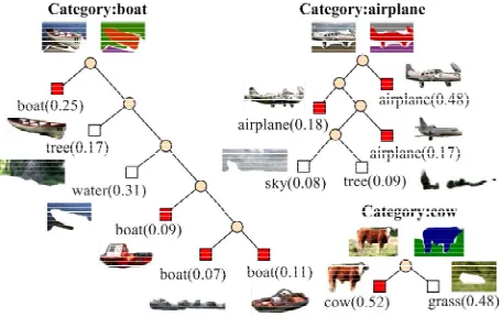
Figure 8 shows some results of the V-PLCA, that is,

object classes for some object categories in a binary tree form. In Figure 8, a typical segment of a class r of each category c is a segment sc i,_j that maximizes p q



c r, sc i,j



.

The mean number of classes per a category for 14 categories was 7.21. Figure 9 shows distance between each

pair of composite probability distributions of key features for all categories which is defined by the expression (18). The mean distance of all pairs of categories was 0.35.

[image:9.595.59.287.503.647.2]

Recognition is performed by computing an object category which gives the minimum distance between composite probability distributions of key features of object categories, which are calculated by the expression (17), and a BoF for an input categorical image according to the following expression

Figure 9. Distance between probability distributions of key features of object categories for two learning sets.

[image:9.595.310.537.665.735.2]

Table 1. Classification accuracy of object categories. Figure 8. Object classes for some object categories in a bi-

nary tree form. A colored square shows that it is an object class of a given category and a white square shows that it is a co-occurring categorical object class in context. A value in a parenthesis represents a class probability and a typical segment of each class is depicted beside the class. A repre- sentative co-occurring segment of each category is also de- picted above a tree.

Samples for recognition A region for

calculating a BoF _{Test samples} _{Training samples}

Co-occurring segments 0.766 0.929

(10)

images was the highest of the four settings for recognition. Thus, it was confirmed that extraction of co-occurring segments from images was effective for recognition through learning by our method.

5. Discussion

The proposed attention-guided organized perception selects an object segment with its contextual segments based on their saliency and the proposed V-PLCA learns a probabilistic structure of appearance features of categorical objects in context from those segments for object category recognition. The distinguished characteristic of the attention-guided organized perception is that spatial preattention is integrated into object-based selective attention for organized perception through segmentation on dynamically-formed MRFs. In the V-PLCA, the number of object classes in object categories is not necessary to be fixed in advance and is determined dependent on learning samples. This characteristic makes it easy to adapt to various features and data sets for learning with- out tuning size parameters of the method.

In experiments of learning through attention-guided organized perception using the Caltech-256 image data set and learning from co-occurring segments using the MSRC labeled image data set v2, it was confirmed that the probabilistic structure of appearance features of objects with context distinctively characterized object categories. It was also confirmed that extraction of co-occurring segments was effective for recognition by show- ing that classification accuracy was higher when using features of co-occurring segments than when using features of entire images through experiments using the MSRC labeled image data set v2. By the way, recognition performance depends on not only learning and recognition methods but also feature coding and pooling methods and learning data sets [32]. The performance of our method is relatively high in comparison with existing methods which used SIFT-based features and the MSRC data set [25,26]. These results demonstrate that our categorical object learning achieves high recognition performance by using co-occurring segments extracted through attention-guided organized perception.

6. Conclusion

We have proposed a probabilistic model of learning object categories through attention-guided organized perception. In this model, a probabilistic structure of object categories is learned and used for recognition based on the probabilistic latent component analysis with the variable number of classes, which uses co-occurring segments extracted through the attention-guided organized perception on dynamically-formed Markov random fields.

Through experiments using images of plural categories in the Caltech-256 image data set and the MSRC labeled image data set v2, it was demonstrated that, by the attention-guided organized perception, our method extracted a set of co-occurring segments which consisted of objects and their context and that, from those co-occurring segments, our method learned a probabilistic structure which represented intra-categorical composition of objects and distinguished inter-categorical difference of objects. It was also confirmed that our method achieved high recognition performance of object categories.

7. Acknowledgements

This work was supported in part by Grant-in-Aid for Scientific Research (C) No.23500188 from Japan Society for Promotion of Science.

REFERENCES

[1] U. Neisser, “Cognitive Psychology,” Prentice Hall, Upper Saddle River, 1967.

[2] M. C. Mozer and S. P. Vecera, “Space- and Object-Based Attention,” In: L. Itti, G. Rees and J. K. Tsotsos, Eds.,

Neurobiology of Attention, 2005, pp. 130-134.

doi:10.1016/B978-012375731-9/50027-6

[3] R. Kimchi, Y. Yeshurun and A. Cohen-Savransky, “Auto- matic, Stimulus-Driven Attentional Capture by Objec-thood,” Psychonomic Bulletin & Review, Vol. 14, No. 1,

2007, pp. 166-172. doi:10.3758/BF03194045

[4] S. Z. Li, “Markov Random Field Modeling in Image Analysis,” Springer-Verlag, Tokyo, 2001.

doi:10.1007/978-4-431-67044-5

[5] T. Hofmann, “Unsupervised Learning by Probabilistic Latent Semantic Analysis,” Machine Learning, Vol. 42,

No. 1-2, 2001, pp. 177-196. doi:10.1023/A:1007617005950

[6] M. Shashanka, B. Raj and P. Smaragdis, “Probabilistic Latent Variable Models as Nonnegative Factorizations,”

Computational Intelligence and Neuroscience, Vol. 2008,

2008, 9 Pages. doi:10.1155/2008/947438

[7] G. Csurka, C. Bray, C. Dance and L. Fan, “Visual Cate-gorization with Bags of Keypoints,” Proceedings of ECCV Workshop on Statistical Learning in Computer Vision,

Prague, 15 May 2004, pp. 1-22.

[8] D. G. Lowe, “Distinctive Image Features from Scale- Invariant Keypoints,” International Journal of Computer Vision, Vol. 60, No. 2, 2004, pp. 91-110.

doi:10.1023/B:VISI.0000029664.99615.94

[9] L. Itti, C. Koch and E. Niebur, “A Model of Saliency- Based Visual Attention for Rapid Scene Analysis,” IEEE Transactions on Pattern Analysis and Machine Intelli- gence, Vol. 20, No. 11, 1998, pp. 1254-1259.

doi:10.1109/34.730558

(11)

pp. 2001, pp. 194-203. doi:10.1038/35058500

[11] S. Frintrop, “VOCUS: A Visual Attention System for Ob- ject Detection and Goal-Directed Search,” Lecture Note in Artificial Intelligence, Vol. 3899, 2006.

doi:10.1007/11682110

[12] M. Atsumi, “Stochastic Attentional Selection and Shift on the Visual Attention Pyramid,” Proceedings of the 5th International Conference on Computer Vision Systems,

Bielefeld, 21-24 March 2007, 10 Pages doi:10.2390/biecoll-icvs2007-32

[13] S. Frintrop, E. Rome and H. I. Christensen, “Computa-tional Visual Attention Systems and Their Cognitive Foundations: A Survey,” ACM Transactions on Applied Perception, Vol. 7, No. 1, 2010, pp. 1-39.

doi:10.1145/1658349.1658355

[14] J. K. Tsotsos and A. Rothenstein, “Computational Models of Visual Attention,” Scholarpedia, Vol. 6, No. 1, 2011. doi:10.4249/scholarpedia.6201

[15] S. Geman and D. Geman, “Stochastic Relaxation, Gibbs Distributions, and the Bayesian Restoration of Images,”

IEEE Transactions on Pattern Analysis and Machine In- telligence, Vol. 6, No. 6, 1984, pp. 721-741.

doi:10.1109/TPAMI.1984.4767596

[16] M. Atsumi, “Attention-Based Segmentation on an Image Pyramid Sequence,” Lecture Notes in Computer Science, Vol. 5259, 2008, pp. 625-636.

doi:10.1007/978-3-540-88458-3_56

[17] T. Liu, Z. Yuan, J. Sun, J. Wang, N. Zheng, X. Tang and H. Y. Shum, “Learning to Detect a Salient Object,” IEEE Transactions on Pattern Analysis and Machine Intelli- gence, Vol. 33, No. 2, 2011, pp. 353-367.

doi:10.1109/TPAMI.2010.70

[18] A. Bosch, A. Zisserman and X. Munoz, “Scene Classifi- cation via pLSA,” Proceedings of the European Confer- ence on Computer Vision, Vol. 3954, 2006, pp. 517-530.

doi:10.1007/11744085_40

[19] S. Huang and L. Jin, “A PLSA-Based Semantic Bag Gen- erator with Application to Natural Scene Classification under Multi-Instance Multi-Label Learning Framework,” 5th International Conference on Image and Graphics, Xi’an, 20-23 September 2009, pp. 331-335.

doi:10.1109/ICIG.2009.108

[20] M. Atsumi, “Learning Visual Object Categories and Their Composition Based on a Probabilistic Latent Variable Model,” Lecture Notes in Computer Science, Vol. 6443, 2010, pp. 247-254. doi:10.1007/978-3-642-17537-4_31 [21] D. Walther, U. Rutishauser, C. Koch and P. Perona, “Se-

lective Visual Attention Enables Learning and Recogni- tion of Multiple Objects in Cluttered Scenes,” Computer

Vision and Image Understanding, Vol. 100, No. 1-2,

2005, pp. 41-63. doi:10.1016/j.cviu.2004.09.004

[22] M. Bar, “Visual Objects in Context,” Nature Reviews Neuroscience, Vol. 5, No. 8, 2004, pp. 617-629.

doi:10.1038/nrn1476

[23] A. Torralba, “Contextual Priming for Object Detection,”

International Journal of Computer Vision, Vol. 53, No. 2,

2003, pp. 169-191. doi:10.1023/A:1023052124951 [24] J. Sivic, B. C. Russell, A. A. Efros, A. Zisserman and W.

T. Freeman, “Discovering Objects and Their Location in Images,” 10th IEEE International Conference on Com- puter Vision, Vol. 1, 2005, pp. 370-377.

doi:10.1109/ICCV.2005.77

[25] A. Rabinovich, C. Vedaldi, C. Galleguillos, E. Wiewiora and S. Belongie, “Objects in Context,” IEEE 11th Inter- national Conference on Computer Vision, Rio de Janeiro,

14-21 October 2007, pp. 1-8. doi:10.1109/ICCV.2007.4408986

[26] C. Galleguillos, A. Rabinovich and S. Belongie, “Object Categorization Using Co-Occurrence, Location and Ap- pearance,” IEEE Conference on Computer Vision and Pat- tern Recognition, Anchorage, 23-28 June 2008, pp. 1-8.

doi:10.1109/CVPR.2008.4587799

[27] M. J. Choi, A. Torralba and A. S. Willsky, “A Tree-Based Context Model for Object Recognition,” IEEE Transac- tions on Pattern Analysis and Machine Intelligence, Vol.

34, No. 2, 2012, pp. 240-252. doi:10.1109/TPAMI.2011.119

[28] M. Atsumi, “Learning Visual Categories Based on Prob-abilistic Latent Component Models with Semi-Supervised Labeling,” GSTF International Journal on Computing,

Vol. 2, No. 1, 2012, pp. 88-93.

[29] J. Zhang, “The Mean Field Theory in EM Procedures for Markov Random Fields,” IEEE Transactions on Signal Processing, Vol. 40, No. 10, 1992, pp. 2570-2583.

doi:10.1109/78.157297

[30] G. Shlomo, “K-tree; A Height Balanced Tree Structured Vector Quantizer,” Proceedings of the 2000 IEEE Signal Processing Society Workshop Neural Networks for Signal Processing X, Sydney, 11-13 December 2000, pp. 271- 280. doi:10.1109/NNSP.2000.889418

[31] G. Griffin, A. Holub and P. Perona, “Caltech-256 Object Category Dataset,” Technical Report 7694, California In- stitute of Technology, Pasadena, 2007.

[32] Y. L. Boureau, F. Bach, Y. LeCun and J. Ponce, “Learn- ing Mid-Level Features for Recognition,” IEEE Confer- ence on Computer Vision and Pattern Recognition, San