Munich Personal RePEc Archive
Practically Implementable Auction for a
Good with Countervailing Positive
Externalities
Bhirombhakdi, Kornpob and Potipiti, Tanapong
Chulalongkorn University
29 November 2012
Online at
https://mpra.ub.uni-muenchen.de/43609/
Practically Implementable Auction for an
Object with Countervailing-Positive
Externalities
Kornpob Bhirombhakdi
Ph.D. candidate, Faculty of Economics, Chulalongkorn University, Thailand [email protected]
Tanapong Potipiti
Faculty of Economics, Chulalongkorn University, Thailand. [email protected]
Revised on 7 Jan 2013
Abstract
This study theoretically presents a new auction design called "take-or-give auction." Unlike in basic auction, the take-or-give auction imposes new rules which the bidders compete for their desired allocation of the object. The auction solves the free-rider problem when applied to an object with countervailing-positive externalities. It is efficient. Moreover, by adding more rules including entry-fee rule, no sale condition and pooling rule, the extended take-or-give auction is the revenue-maximizing auction.
1. Introduction
As found in the previous literature, the basic auctions -- first- and second-price sealed-bid auctions -- for an object with positive externalities are most likely to fail for efficient allocation or revenue maximizing since the existence of free-rider problem (Jehiel and Moldovanu, 2000; Bagwell, Mavroidis and Staiger, 2007). This study proposes a new auction "take-or-give with second-price payment" that solves the problem. The analysis shows that the new auction is efficient and its extended version maximizes expected revenue.
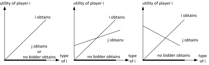
externalities which is a special case. The countervailing positive externalities is a kind of type-dependent-positive externalities which the effects on non-obtainer negatively relate with his type, which represents the payoffs gained if he is the obtainer. Precisely, the higher type is the more payoffs if being the obtainer but the less positive effects (or the less payoffs) from the obtainer's consumption if being a non-obtainer. For instance, Figure 1 (on the right) graphically presents the utility function on a countervailing-positive-externalities object which a bidder has increasing utility in his type if being the obtainer; but decreasing if other player is the obtainer and he is a non-obtainer; while if nobody obtains the object (or the seller keeps it) he gets zero payoff as status quo. Notice that the non-obtainer's utility is positive for any type because of the positive externalities. To compare the differences, Figure 1 presents the utility function on a normal object (on the left) and an object with non-countervailing positive externalities (in the middle).
The following exhibit can be a good example for the countervailing-positive-externalities object. Think of two adjacent towns -- A and B -- competing for a new airport to be built in one town. Precisely, the government has a budget to build one airport in town A or B. The town bares no cost of building the airport but bares the maintenance costs of tourist attractions. Each town has its own number of tourist attractions which is exogenously given by nature (e.g. by geography of the town). The number of attractions represents the town's type. In the airport town (the town which obtains the airport), there will be economic boom which the more attractions the more profit (or payoffs) is gained (since the average revenue per attraction is higher than the average maintenance cost) -- the obtainer has increasing payoffs in its type. In the non-airport town, since it is close to the airport town it will get quite substantial revenue from spillover effects of the economic boom. In other words, for any type of the non-airport town, the town always gets positive profit. Suppose that the economic boom provide fixed lump-sum revenue for the non-airport town. The non-airport town gets the highest profit when it has no attraction. While, given that the average maintenance cost is constant in the number of attractions, since the average revenue is decreasing in the number, the profit is decreasing as well. Therefore, in this exhibit the airport shows the countervailing-positive-externalities property. 1
Like the case of public good provision in which the contributor with low marginal benefits from his contribution -- or low type -- avoids contributing in the provision since he wants to do the free ride on others' contributions, in any basic auction the bidder with low type avoids participating to compete for the object with positive externalities since he wants to do the free ride on the obtainer's consumption. The main cause of such the failure is that, the basic auction sets the rules which the highest-bid bidder pays and obtains the object hence it does not provide proper incentives for low-type bidders who does not want to pay nor obtain it. Therefore, a new type of auction which solves the problem must be implemented.
The following in this article, it starts with reviews related literature (in section 2.), presents the model, numerical application and the revenue-maximizing target (in section 3.), presents the free-rider problem in second-price sealed-bid auction, the take-or-give auction, the take-or-give auction with revenue-enhancing rule I and the take-or-give auction with revenue-enhancing rule II (respectively in section 4-7.). Last section concludes.
1
We may mathematically express as ( ) (where is the total cost, is the average variable cost per unit of attractions and is type, or the number of attractions), ( ) (where is the total revenue of the airport town, is the fixed revenue which and is the average revenue per unit of attractions such that ) and
(where is the total revenue of the non-airport town and is the lump-sum revenue from economic
no bidder obtains type
of i utility of player i
i obtains
j obtains or
no bidder obtains type
of i i obtains utility of player i
j obtains
utility of player i
i obtains
type of i no bidder obtains
[image:4.612.144.479.74.179.2]j obtains
Figure 1 Utility Function for a Normal Object (on the left), an Object with Non-Countervailing-Positive Externalities (in the middle) and With Countervailing-Positive Externalities (on the right)
2. Literature Review
Related to this study, Jehiel, Moldovanu and Stacchetti (1996), Jehiel and Moldovanu (2000), Bagwell, Mavroidis and Staiger (2007), Brocas (2007) and Chen and Potipiti (2010) are interesting literature which is related with auction design for an object with externalities. Moreover, Lewis and Sappington (1989) relates since this study deals with countervailing-positive externalities and countervailing incentives.
Jehiel et al. (1996), Jehiel and Moldovanu (2000) and Brocas (2007) studied various cases of negative externalities -- a non-obtainer gets negative payoffs from negative-effect consumption of the obtainer. Jehiel et al. (1996) and Brocas (2007) shared the similar feature of finding revenue-maximizing auction. In their optimal auctions, they provided two interesting discussions. First, the optimal auction should have rules which put threats on nonparticipating bidders to get the lowest possible payoffs; as consequences, all potential bidders will participate in the auction and the seller will get higher expected revenue. In the case of negative externalities, the rule is to promises selling the object to some participating bidders; hence a nonparticipating bidder will always get negative payoff. Even in the case of normal object -- without externalities -- where the revenue-maximizing mechanism shown in Myerson (1981) is the second-price sealed bid auction with reservation price, it puts the same rule that some participating bidders always obtain the object; hence nonparticipating bidders always get the lowest possible payoff at zero payoff as status quo.
Second, in the case of negative externalities, the studies found that the seller can extract non-obtainers' surplus; in other words, in the optimal auction the non-obtainers pay some amount. Precisely, since the non-obtainers have incentives to pay for preventing selling the object, the seller can extract surplus (from payment) from them. For instance, if a bidder gets -6$ when being non-obtainer and gets 0 payoff when nobody being obtainer, he is willing to pay up to 6$ to convince the seller to keep the object.
According to the second discussion, Jehiel and Moldovanu (2000) argued that collecting payment from any non-obtainer the rule is incredible. Hence, the study studied standard auction which has only reservation price and entry fee as its credible rules. However, the standard auction is not an optimal auction.
free-rider problem --occurred in the case of positive externalities. It makes the seller gets less expected revenue since some low-type bidders avoid participating. There has been no study solving the problem.
Chen and Potipiti (2010) studied the optimal auction in the case of countervailing-positive externalities under direct-mechanism setting. It found interesting points as follows:
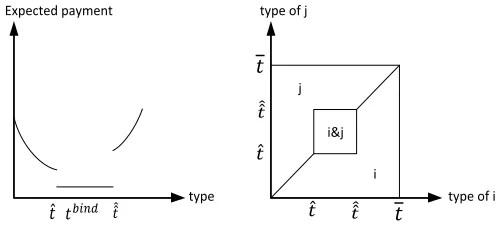
i) The optimal mechanism selects the binding type -- the type which get zero utility (as status quo) from the mechanism -- interiorly. Precisely, unlike the case of normal object where the binding type is the lowest type, the binding type in the study is in between the lowest and highest types. Figure 2 presents the expected payment and allocation in the optimal mechanism of the study. The binding type is
which is interior.
ii) There are some types around the binding type are pooled together with the binding type. As presented in the figure, ( ̂ ̂̂) is the pooling region. Hence, a bidder with any type in the region has the same expected payment. Also, in the case of two bidders studied by the study, if both bidders have types in the region, each bidder has 0.5 chance of being obtainer; this is the consequence of pooling characteristics.
iii) The optimal mechanism provides countervailing incentives.2 As a consequence, as presented in the figure, the expected payment is non-monotonic in type.
iv) In the optimal mechanism, if payoffs of bidders are high enough, all types have some expected payment and there is no chance of not selling (see Figure 2 on the right). The results imply that there is no free-rider problem and bidders always participate in the auction.
Moreover, like Chen and Potipiti (2010), Brocas (2007) also showed in the case of negative externalities that under some circumstances the optimal auction provided countervailing incentives by selecting the interior binding type and pooling its neighbors. Lewis and Sappington (1989), which studied principal-agent problem with existence of externalities, found the similar results.
Even Chen and Potipiti (2010) successfully characterized the optimal auction for an object with countervailing-positive externalities, since the study was conducted under the direct-mechanism setting, the study did not show that what the practically implementable auction should be. Hence, this study aims to extend from the study by proposing practically implementable auction for an object with countervailing-positive externalities.
2
Expected payment
type
type of j
type of i i&j
[image:6.612.180.432.74.188.2]i j
Figure 2 Expected Payment and Allocation of the Optimal Mechanism.
3. The Model, Numerical Application and
Revenue-Maximizing Target
In this study, it applies the same model as in Chen and Potipiti (2010) for the case of countervailing-positive-externalities object. There are two risk neutral and symmetric bidders * +. They compete in an auction for an indivisible object with countervailing positive externalities. The object has no value to the seller.
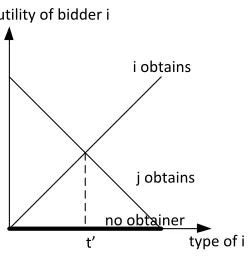
Denote and as the index of bidder. Bidder i's type is randomly drawn from
[ ] with distribution function and its associated density function which ( ) for all . As presented in Figure 3, his payoff which depends on his type and the ex-post outcome is defined by
( ) { ( ( ) )
( )
where and is high enough to make ( ) ( ) for . Assume that which yields a solution ( ) ( ) (Assumption 1).
ASSUMPTION 1
and there is a solution ( ) ( ).
To be able to compare expected revenue from auctions in the following analyzes with the optimal target, this study also takes the same numerical application from Chen and Potipiti (2010). The application was set for the case of selling retaliation rights in the WTO.
type of i utility of bidder i
i obtains
[image:7.612.246.372.73.206.2]j obtains no obtainer t’
Figure 3 Bidder's Utility Function.
[
( ) ( )
( )
]
( )
For the details of the application, this section refers readers who are interested to Chen and Potipiti (2010). Here, as presented in (2), it simply and numerically presents the final variables equivalent to the model (1).
Under the application specification, Chen and Potipiti (2010) also derived for the optimal revenue. It is the revenue-maximizing target which we will compare it with the expected revenue gained from other auctions in the following sections. The revenue-maximizing target is also presented in (2).
4. Free-Rider Problem in Second-Price Sealed-Bid
Auction
PROPOSITION 1
( ) , [ ̃)
[ ̃ ] ( ) ,
[ ) ( ) ( ) [ ]
where ̃ and ̃ solves
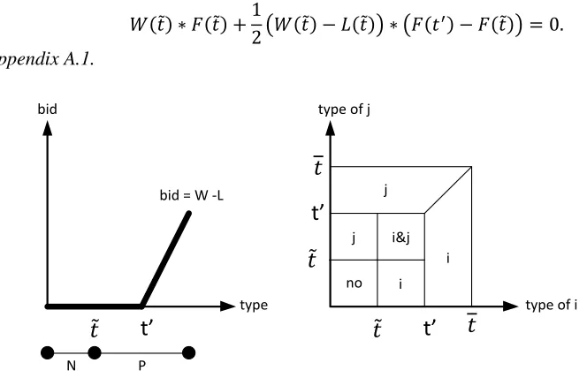
( ̃) ( ̃) ( ( ̃) ( ̃)) ( ( ) ( ̃)) ( )
Proof: See Appendix A.1.
t’
bidtype bid = W -L
t’
type of jtype of i
t’
no i j i&j
i j
[image:8.612.131.463.135.349.2]N P
Figure 4 Symmetric-Equilibrium Strategy and Allocation in Second-Price Sealed-Bid Auction. (no = no obtainer, i = i obtains, j = j obtains, i&j = each bidder has 0.5 chance of being obtainer)
According to the proposition, Figure 4 presents symmetric-equilibrium strategy (on the left) and allocation (on the right) in second-price sealed-bid auction. On the left, Y-axis is bid, X-axis is type and the line under X-axis notifies participating (P) or not participating (N) at each corresponding type. On the right, X and Y axes are types of both bidders.
The equilibrium strategy shows the existence of free-rider problem. Precisely, the free rider is a bidder with type [ ) who gets higher utility from being non-obtainer ( ) ( ) from being obtainer. He avoids participating in the auction (for type [ ̃)) or participating with zero bid (for type , ̃ )). The type ̃ is the type which feels indifferent between not participating or participating with zero bid.
Next, we compare the expected revenue of the second-price sealed-bid auction with of the optimal target in (2). According to the proposition, the expected revenue of the second-price sealed-bid auction is
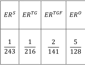
By applying the numerical application in (2), it gets . Hence,
. The
second-price sealed-bid auction is not the revenue-maximizing auction.3
5. Take-or-Give Auction with Second-Price Payment
This section proposes a new auction called "take-or-give auction with second-price payment." It is the efficient auction for an object with countervailing positive externalities (Corollary 1). In this section, it starts with simple illustration under two discrete types and perfect information. In the illustration, the rules of the new auction are discussed and informal analysis shows that the auction fixes the free-rider problem. Then, section 5.2. analyzes for the symmetric-equilibrium strategy in the auction and compares the expected revenue with the optimal target.5.1. Simple Illustration
Since any basic auction fails to be optimal since it does not provide the proper incentives for bidders who have utility from being non-obtainer ( ) ( ) from being obtainer, the free-rider problem happens. Hence, this study proposes a new auction which can fix the problem by providing the proper incentives -- allowing the highest-bid bidder select for himself his desired allocation. In other words, instead of always obtaining the object, the new auction lets the highest-bid bidder chooses whether to take the object and be the obtainer or to give the object to his opponent and be the non-obtainer. The new auction is "take-or-give auction with second-price payment."
The take-or-give auction allows each bidder submit a doublet which composes of bid and the demand of allocation of the object. The demand can be either to take and be the obtainer or to give his opponent the object (for free as a gift) and be a non-obtainer.
The payment is the second-price payment conditioned on their demands. Precisely, if both bidders submit the same demand, the highest-bid bidder pays his opponent's bid as the second price. Or if both bidders submit different demands, they pay nothing (as a zero reservation price conditioned on each demand).
The allocation is done as the highest-bid bidder's demand; if he demands to take then he obtains the object; if he demands to give then he gives his opponent the object. Note that he gives it as a gift, gives it for free; the receiver pays nothing, obtains the object and voluntarily decides whether to consume
3
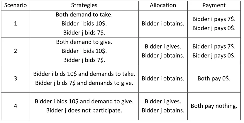
Table 1 Examples for Allocation and Payment Mechanisms in Take-or-Give Auction with Second-Price Payment.
Scenario Strategies Allocation Payment
1
Both demand to take. Bidder i bids 10$.
Bidder j bids 7$.
Bidder i obtains. Bidder i pays 7$. Bidder j pays 0$.
2
Both demand to give. Bidder i bids 10$.
Bidder j bids 7$.
Bidder i gives. Bidder j obtains.
Bidder i pays 7$. Bidder j pays 0$.
3 Bidder i bids 10$ and demands to take.
Bidder j bids 7$ and demands to give. Bidder i obtains. Both pay 0$.
4 Bidder i bids 10$ and demand to give.
Bidder j does not participate.
Bidder i gives.
Bidder j obtains. Both pay nothing.
or not. Also, notice that optimally the receiver voluntarily consumes the object and the giver gets positive externalities.4
The Table 1 presents four scenarios as examples for allocation and payment mechanisms in take-or-give auction with second-price payment. In the 1st and 2nd scenario, if the highest-bid bidder submits the same demand as his opponent's, he pays the second price and allocates the object as his demand. In the 3rd and 4th scenarios, respectively, if the highest-bid bidder submits different demand as his opponent's or his opponent does not participate, he allocates the object as his demand without payment.
ASSUMPTION 2
If potential bidders know the auction rules prior to their participations, a credible auction can collect payment from participating bidders but cannot collect payment from nonparticipating ones.
ASSUMPTION 3
The seller can allocate the object to any nonparticipating bidder.
Notice that i) the auction can collect payment from non-obtainer but cannot collect it from nonparticipating bidder. According to Jehiel and Moldovanu (2000) which argued that collecting payment from non-obtainer the rule is incredible, this study differently puts that a credible auction can collect payment from any participating bidders (including both obtainer and non-obtainers) but cannot collect it from any nonparticipating bidders (Assumption 2); since all potential bidders know the auction rules before deciding to participate or not, their participations imply that they accept the rules and imply that they are willing to pay under some possible outcomes that they are non-obtainers.
4
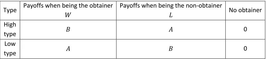
Table 2 Payoffs of Two Discrete Types Illustration. ( ).
Type Payoffs when being the obtainer Payoffs when being the non-obtainer No obtainer
High
type 0
Low
type 0
ii) Unlike in the basic auction, in the take-or-give auction the seller can allocate the object to any nonparticipating bidders (without payment) (Assumption 3). As discussed in Jehiel et al. (1996) that in a feasible auction the seller could not allocate the object to a nonparticipating bidder, the take-or-give auction imposes differently. However, as discussed in Assumption 2, the auction is credible if the nonparticipating bidder gets the object without payment; hence in the take-or-give auction the seller can allocate the object to any nonparticipating bidders for free as giving as a gift.
Precisely, the take-or-give auction with second-price payment is processed in three steps as follows:
1. Each bidder submits his doublet of bid and demand (which is taking or giving).
2. The seller selects the highest-bid bidder's demand and allocates the object accordingly. If the bids are tied, the seller prefers to allocate the object to a bidder who demands to take than to give.
3. The highest-bid bidder pays equal to:
- his opponent's bid if they submit the same demand,
- or zero if his opponent submits different demand or does not participate.
Next, we apply the case of two discrete types and perfect information and analyze for the symmetric-equilibrium strategy in the take-or-give auction with second-price payment. Table 2 presents payoffs of high and low types conditioned on each ex-post outcome. To satisfy the countervailing-positive-externalities property, assume .
In the auction, bidder i has strategy ( ) which * + means that he participates ( ) or does not participate ( ) in the auction, is his bid and * + is demand to take ( ) or demand to give ( ). Under the setting of two discrete types (as presented in the table) and perfect information, by symmetry, each bidder who has symmetric type ( * +) submits his symmetric-equilibrium strategy in the take-or-give auction with second-price payment ( ) as presented in Proposition 2.
PROPOSITION 2
( ) {
5.2. Formal Analysis
This section formally presents the symmetric-equilibrium strategy in take-or-give auction with second-price payment. The equilibrium strategy ( ) is presented in Proposition 3.
PROPOSITION 3
( ) , ( ) ( ) [ ]
( ) ( ) [ ) ( ) ,
[ ] [ )
Proof: See Appendix A.3.
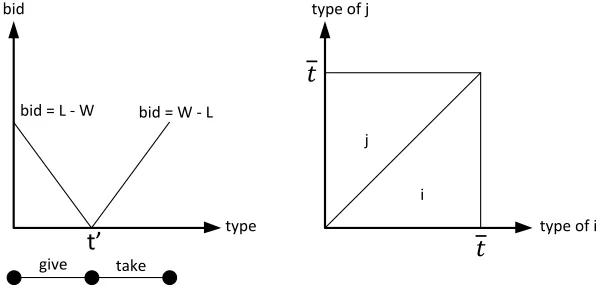
According to the proposition, Figure 5 presents symmetric-equilibrium strategy (on the left) and allocation (on the right) in take-or-give auction with second-price payment. The equilibrium strategy shows that the take-or-give auction fixes the free-rider problem; no bidder avoids participating and they bids according to their willingness to pay. Precisely, a bidder who has utility from being non-obtainer
( ) ( ) from being obtainer (which [ )) participates with demand to give and ( ) ( ) bid as his willingness to pay, and vice versa.
Moreover, the auction is efficient (Corollary 1); since there is no chance of not selling and the highest-type bidder always obtains the object (see Figure 5 on the right).
COROLLARY 1
Take-or-give auction with second-price payment is the efficient auction for an object with countervailing-positive externalities.
Also, notice that the take-or-give auction implicitly has the countervailing-incentive rule. The rule provides countervailing incentives which cause non-monotonic bid. The rule has revenue-enhancing effect. Previous literature which studied the optimal auction for an object with externalities also found that their optimal auctions provided countervailing incentives (Lewis and Sappington, 1989; Brocas, 2007; Chen and Potipiti, 2010).
Next, we compare the expected revenue of the take-or-give auction with of the optimal target
in (2). According to the proposition, the expected revenue of the take-or-give auction is
[∫ ∫ ( ( ) ( )) ( ) ( ) ∫ ∫ ( ( ) ( )) ( ) ( )]
t’
bid
type bid = W - L
type of j
type of i i
j bid = L - W
[image:13.612.155.458.76.224.2]give take
Figure 5 Symmetric-Equilibrium Strategy and Allocation in Take-or-Give Auction with Second-Price Payment.(i = i obtains, j = j obtains).
Table 3 Comparison of Expected Surplus of Take-or-Give Auction with Second-Price Payment.
6. Take-or-Give Auction with Revenue-Enhancing
Rule I: Entry Fees
In the previous section, the take-or-give auction for an object with countervailing-positive externalities solves the free-rider problem and is the efficient auction. However, it is not the revenue-maximizing. As commonly known, the revenue-maximizing auction is most likely to be inefficient auction by imposing more revenue-enhancing rules. The seller does trade-off between the efficiency and revenue.
This chapter introduces entry-fee rule to the take-or-give auction. It is a revenue-enhancing rule which is mostly applied in the case of an object with externalities (Brocas, 2007). As will be presented in this section, the rule has exclusion effect which makes some bidders with low willingness to pay avoid participating. Hence, the auction with the rule is inefficient. However, it yields the expected revenue higher than the auction without it.
6.1. Simple Illustration
This section applies two discrete types and perfect information to be analyzed for the symmetric-equilibrium strategy in the take-or-give auction with entry-fee rule. Precisely, we call the auction "take-or-give auction with second-price payment and entry fees."
Like in a basic auction, the entry-fee rule says that a bidder must pay the fee for participation. The rule can increase the expected revenue -- or revenue-enhancing effect -- but also increase the chance of not participating by some low-willingness-to-pay bidders; hence it decreases the efficiency of an auction. We call the effect "exclusion effect."
In the take-or-give auction with second-price payment and entry fees, the seller designs a menu of entry fees ( ) which a bidder pays if he demands to give; or pays if he demands to take. Notice that the entry-fee rule in this auction has two differentiated entry fees according to demand. It is different from the entry-fee rule in a basic auction that has only one entry fee.
The take-or-give auction with second-price payment and entry fees is processed as follows: 1. Each bidder submits his doublet which composes of bid and entry fee -- if he demands to
take or if he demands to give.
2. The seller selects the highest-bid bidder's demand and allocates the object accordingly. If the bids are tied, the seller prefers to allocate it to a bidder who pays to .
3. The highest-bid bidder additionally pays equal to:
- his opponent's bid if they submit the same entry fee,
- or zero if his opponent submits different entry fees or does not participate.
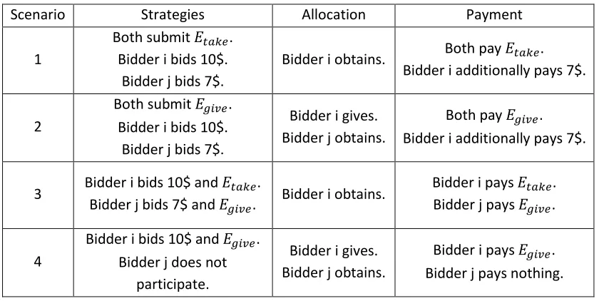
To give some examples of the allocation and payment mechanisms, Table 4 presents four scenarios in take-or-give auction with second-price payment and entry fees. In the 1st and 2nd scenarios, if the highest-bid bidder submits the same fee as his opponent's, he pays the fee and second price and the object is allocated as his demand which is specified with his fee -- demand to give with and demand to take with . In the 3rd and 4th scenarios, respectively, if the highest-bid bidder submits different fee as his opponent's or his opponent does not participate, he pays only the fee and the object is allocated as his demand.
The analysis here applies two discrete types as in previous chapters. Table 2 presents payoffs of each type. In the auction with entry fees, bidder i submits his strategy ( ) which * + means that he participates ( ) or does not participate ( ) in the auction, is his bid and
{ } is the entry fee. For simplicity, assume and .
Under perfect information, by symmetry, each bidder who has symmetric type (
Table 4 Examples for Allocation and Payment Mechanisms in Take-or-Give Auction with Second-Price Payment and Entry Fees.
Scenario Strategies Allocation Payment
1
Both submit . Bidder i bids 10$.
Bidder j bids 7$.
Bidder i obtains. Both pay .
Bidder i additionally pays 7$.
2
Both submit . Bidder i bids 10$.
Bidder j bids 7$.
Bidder i gives. Bidder j obtains.
Both pay . Bidder i additionally pays 7$.
3 Bidder i bids 10$ and .
Bidder j bids 7$ and . Bidder i obtains.
Bidder i pays . Bidder j pays .
4
Bidder i bids 10$ and . Bidder j does not
participate.
Bidder i gives. Bidder j obtains.
Bidder i pays . Bidder j pays nothing.
PROPOSITION 4
( ) {
where and .
Proof: See Appendix A.4.
From the equilibrium strategy, notice that i) the exclusion effect makes the chance of not participating (N) in either type realization. Precisely, the probability of not participating implies that the effect positively depends on the entry fee . Because of the exclusion effect, there is . / chance that the seller keeps the object. Compared with the auction without the fees, it is inefficient.
ii) The entry-fee rule (at proper level) does not affect bidding behavior. Precisely, bidding strategy in equilibrium of the auction with fees and of the auction without fees (see Proposition 2) are equal . Also, iii) a bidder with high type has demand to take by submitting and a bidder with low type has demand to give by submitting . It is the same as in the auction without fees.
6.2. Formal Analysis
This section formally presents the symmetric-equilibrium strategy in take-or-give auction with second-price payment and entry fees under continuous types and imperfect information. Then, it compares the expected revenue from the auction and optimal target.
PROPOSITION 5
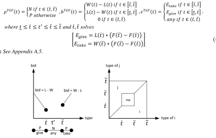
( ) { ( ̇ ̈)
( ) {
( ) ( ) [ ̈ ] ( ) ( ) [ ̇]
( ̇ ̈)
( ) { [ ̈ ] [ ̇]
( ̇ ̈)
where ̇ ̈ and ̇ ̈ solves
* ( ̇) ( ( ̈) ( ̇))
( ̈) ( ( ̈) ( ̇))+ ( )
Proof: See Appendix A.5.
t’
bidtype bid = W - L
type of j
type of i bid = L - W
give any take
P N P
no
[image:16.612.99.531.111.388.2]i j
Figure 6 Symmetric-Equilibrium Strategy and Allocation in Take-or-Give Auction with Second-Price Payment and Entry Fees. (i = i obtains, j = j obtains, no = no obtainer).
According to the proposition, Figure 6 presents symmetric-equilibrium strategy (on the left) and allocation (on the right) in take-or-give auction with second-price payment and entry fees. The equilibrium strategy shows that the take-or-give auction with entry fees has exclusion effects on both sides (demand-to-take and demand-to-give sides) which make it be inefficient auction. The effect makes some low-willingness-to-pay bidders (whose types are around ) avoids participating. Precisely, by the entry fee (given some ), there is a type ̇ which is the binding type (the type which gets expected surplus as its reservation price, or zero surplus) on the giving side. Similarly, by the entry fee (given some ) there is a type ̈ which is the binding type on the taking side. The types in ( ̇ ̈) are excluded from the auction with ( ) entry fees.
Moreover, Notice that i) if , the auction is equivalent to the one without entry fees. ii) There no solution which entry fee on one side is zero and the other side is positive (e.g.
); hence both fees are simultaneously positive. iii) The entry fees do not affect bidding behavior
of bidders who participate. This is different from introducing reservation-price rule which will affect bidding behavior.5
5
reservation-Next, we compare the expected revenue of the take-or-give auction with entry fees to of the auction without fees, of the second-price sealed-bid auction and of the optimal target. According to the proposition, the expected revenue of the take-or-give auction with entry fees is
[∫ *
∫ ( ( ) ( )) ( ) ̇
+ ( )
̇
∫ * ∫ ( ( ) ( )) ( )
̈ + ( )
̈ ]
According to the equilibrium strategy which is induced by the menu of entry fees ( ), the seller designs optimal menu ( ) that maximizes his expected revenue by solving the Problem 1.
PROBLEM 1
[
( ̇) ( ( ̈) ( ̇)) ( ̈) ( ( ̈) ( ̇))]
By applying the numerical application in (2), the optimal menu has the solution as
( ) . /. Hence, at optimal . It is higher than the expected revenue of
the auction without fees and second-price sealed-bid auction but still less than the optimal target . Table 5 compares the expected revenue among auctions.
7. Take-or-Give Auction with Revenue-Enhancing
Rule II: Entry Fees, No Sale Condition and Pooling
Rule
This section introduces a set of revenue-enhancing rules including entry-fee rule, no sale condition (which the auction is cancelled if any potential bidder does not participate) and pooling rule (which allows bidders to participate without specifying their demands) to the take-or-give auction. Interestingly, the auction with the set of rules is the revenue-maximizing auction.
In this section, it starts with simple illustration under four discrete types and imperfect information (in section 7.1.) and formally analyzes for the symmetric-equilibrium strategy and expected revenue (in section 7.2.).
Table 5 Comparison of Expected Surplus of Take-or-Give Auction with Second-Price Payment and Entry Fees.
7.1. Simple Illustration
In the illustration, it aims to present that with the no sale condition and pooling rule the auction is the revenue maximizing. To show the issue, we compare the expected revenue from the auction with the set of rules and from the auction without pooling rule (only entry-fee rule and no sale condition are introduced).
The no sale condition is the rule which states that the auction will be cancelled if any potential bidder does not participate. Opposite to the entry-fee rule, the condition has inclusion effect. Precisely, recall that the take-or-give auction with entry fees (without no sale condition) has interval ( ̇ ̈) which avoids participating (see Proposition 5), the nonparticipating bidders get positive expected utility from the positive externalities. With the condition, the bidders with types in the interval will participate to prevent the cancellation. The effect increases both participation rate and expected revenue.
The pooling rule allows bidders to participate without specifying their demands. If there is no bidder participates with specific demand (to take or to give), regardless of their bids, the pooled bidders have equal chance of being obtainer. Precisely, with the pooling rule, the seller designs a menu of entry fees ( ) which a bidder who demands to take will submit ; a bidder who demands to give will submit ; a bidder who does not want to specify his demand (or to be "pooled") will submit . Notice that, with a proper design, the is good for any bidder who participates to prevent the cancellation of auction.
Table 6 presents seven scenarios as examples for allocation and payment mechanisms in take-or-give auction with second-price payment, entry fees, no sale condition and pooling rule. In the 1st-5th scenarios, there is some bidders who are no pooled. The highest-bid bidder who is not pooled pays the fee and the object is allocated according to the fee. He pays the second price if his opponent submits the same fee. In the 6th scenarios, all bidders are pooled, regardless of their bids, the object is randomly allocated with equal probability and bidders pay only the fees. In the 7th scenario, the auction is cancelled if some bidders do no participate, bidders pay nothing.
Table 6 Examples for Allocation and Payment Mechanisms in Take-or-Give Auction with Second-Price Payment, Entry Fees, No Sale Condition and Pooling Rule.
Scenario Strategies Allocation Payment
1
Both submit . Bidder i bids 10$.
Bidder j bids 7$.
Bidder i obtains. Both pay . Bidder i additionally pays 7$.
2
Both submit . Bidder i bids 10$.
Bidder j bids 7$.
Bidder i gives. Bidder j obtains.
Both pay . Bidder i additionally pays 7$.
3 Bidder i bids 10$ and .
Bidder j bids 7$ and . Bidder i obtains.
Bidder i pays . Bidder j pays .
4 Bidder i bids 10$ and .
Bidder j bids 7$ and . Bidder i obtains.
Bidder i pays . Bidder j pays .
5 Bidder i bids 10$ and . Bidder j bids 7$ and .
Bidder i gives. Bidder j obtains.
Bidder i pays . Bidder j pays .
6
Both submit . Bidder i bids 10$.
Bidder j bids 7$.
0.5 chance to obtain. Both pay .
7 Bidder i bids 10$ and .
Bidder j does not participate. Nobody obtains. Both pay nothing.
1. Each bidder submits his doublet which composes of bid and entry fee -- if he demands to take, if he demands to give or if he demands to be pooled. Not participating is also available which if any bidder does so both pay nothing and the auction is cancelled. 2. If the auction is not cancelled, the seller selects the highest-bid bidder who submits or
and allocates the object according to his demand. If the highest-bid bidder submits but the other does not submit , then allocate the object according to the
demand of the bidder who does not submit . If the bids are tied, the seller prefers to allocate it to a bidder who pays than and than (and the transitivity holds).
3. The highest-bid bidder additionally pays equal to:
- his opponent 's bid if they submit the same entry fee or , - or zero if his opponent submits different entry fee.
Table 7 Payoffs of Four Discrete Types Illustration. ( )
Type Payoffs when being the obtainer Payoffs when being the non-obtainer No obtainer High
(H) 10 0 0
Middle 1
(N) 0
Middle 2
(M) 0
Low
(L) 0 10 0
In this illustration, there are two risk-neutral and symmetric bidders whose types are independently and randomly drawn from * +. The type has uniform distribution. Bidder i has his strategy ( ) which * + means that he participates ( ) or does not participate ( ) in the auction, is his bid and { } is the entry fee.
In the take-or-give auction with second-price payment, entry fees, no sale condition and pooling rule, the seller designs ( ) and the auction rules as discussed previously. Recall that the entry fees have exclusion effects while the no sale condition has inclusion effects. With a proper design, the inclusion effects dominate the exclusion effects.6 In other words, all bidders participate in the auction. On the opposite, if it is not properly designed, the exclusion effects dominate the inclusion effects and some bidders avoid participating. We assume that the seller is interested in designing the auction in which all bidders participate (Assumption 4).
ASSUMPTION 4
The seller designs the auction in which all bidders participate.
Suppose that the seller designs and . The symmetric-equilibrium strategy in the auction ( ) is presented in Proposition 6.
PROPOSITION 6
( ) { * +
* + ( ) {
* +
where and .
Proof: See Appendix A.6.
6
Notice that i) the design and satisfies Assumption 4. ii) The design optimally yields expected revenue since a bidder with any type is left with zero expected surplus.
Next, we will characterize the equilibrium strategy in the auction without pooling rule and will calculate the expected revenue to compare with the revenue in the auction with pooling rule. For the take-or-give auction with second-price payment, entry fees and no sale condition (without pooling rule), the seller designs ( ) and the auction rules are similar to the auction with the pooling rule excepts no to be submitted.
In the auction without pooling rule, bidder i has his strategy ( ) which * + means that he participates ( ) or does not participate ( ) in the auction, is his bid and
{ } is the entry fee. Suppose the seller design ( ). The
symmetric-equilibrium strategy in the auction without pooling rule ( ) is presented in Proposition 7.
PROPOSITION 7
( ) { * +
* + ( ) { * + * +
where ( ).
Proof: See Appendix A.7.
Also notice that the expected revenue of this auction is comparable with the previous one with pooling rule since i) the design ( ) in this auction satisfies Assumption 4 and ii) given this auction rules it optimally yields expected revenue. By comparing the expected revenue from the auction with pooling rule (in Proposition 6) and from the auction without pooling rule (in Proposition 7), it shows that the auction with the pooling rule yields higher revenue than the one without the rule. Hence, in next section where we do the formal analysis, we will directly analyze the auction with pooling rule for its equilibrium strategy and expected revenue.
Intuitively, the pooling rule has two revenue-enhancing effects. Fist, the seller can directly extract payment from some types which participate to prevent the cancellation of auction. Second, the seller can reduce the information rent paid to other non-pooling types. Lewis and Sappington (1989) and Brocas (2007) discussed the second effect.
7.2. Formal Analysis
PROPOSITION 8
( ) { ( ) ( ) [
]
( ) ( ) [ ] ( )
( ) {
[ ] [ ] ( )
where and solves
[
(
)
∫ ( ) ( ) ∫ . ( ) ( )/ ( )
∫ ( ) ( )
∫ ( ( ) ( )) ( )
∫ ( ( ) ( )) ( )
∫ ( ) ( ) ∫ ( ) ( )
∫ ( ) ( )
∫ ( ) ( )
]
( )
Proof: See Appendix A.8.
bid
type bid = W - L
type of j
type of i bid = L - W
give pool take
i&j
i j
t* t** bid = 0
t* t** t*
[image:22.612.89.502.82.504.2]t**
Figure 7 Symmetric-Equilibrium Strategy and Allocation in Take-or-Give Auction with Second-Price Payment, Entry Fees, No Sale Condition and Pooling Rule.(i = i obtains, j = j obtains, i&j = each bidder has 0.5 chance of being obtainer).
According to the equilibrium strategy, Figure 7 presents symmetric-equilibrium strategy (on the left) and allocation (on the right) in take-or-give auction with second-price payment, entry fees, no sale condition and pooling rule. The equilibrium strategy shows that, in the auction, bidders' behaviors are classified into three groups according to the submitted fee. Precisely, the pooling types ( ), they are in the middle region including and some neighbors. They participate with and zero bid. The taking types [ ] are on the taking side (toward the highest type) and participate with and bid as their willingness to pay. Last, the giving types [ ] are on the giving side (toward the lowest type) and participate with and bid as their willingness to pay.
is the type which gets the expected surplus as its reservation utility by paying
while other
pooling types around are left for some surplus. Then, the types and are selected to get the expected surplus as their reservation utility on each side by paying the submitted fee and expected payment from the second price. Other types further than and to each extremity -- to and -- are left for some surplus. Since the seller designs and higher than , the pooling types
( ) cannot deviate to pay
or .
Next, we compare the expected revenue of the auction with the optimal target. According to the proposition, the expected revenue of the take-or-give auction with second-price payment, entry fees, no sale condition and pooling rule is
[∫ *
∫ ( ( ) ( )) ( )+ ( ) ∫ ( )
∫ * ∫ ( ( ) ( )) ( )
+ ( )
]
According to the equilibrium strategy which is induced by the menu of entry fees
( ), the seller designs optimal menu ( ) that maximizes his
expected revenue by solving the Problem 2.
PROBLEM 2
[
( )
]
By applying the numerical application in (2), the optimal menu has the solution as
( ) . /. Hence, at optimal . It is equal to the optimal
target . Table 8 compares the expected revenue of previously analyzed auctions.
Analytically, the auction is equivalent to the optimal mechanism characterized in Chen and Potipiti (2010). Hence, the take-or-give auction with second-price payment, entry fees, no sale condition and pooling rule is the revenue-maximizing auction (Proposition 9).
PROPOSITION 9
The take-or-give auction with second-price payment, entry fees, no sale condition and pooling rule is the revenue-maximizing auction for an object with countervailing- positive externalities.
Proof: See Appendix A.9.
Table 8 Comparison of Expected Surplus of Take-or-Give Auction with Second-Price Payment, Entry Fees, No Sale Condition and Pooling Rule.
[image:24.612.110.495.397.512.2]
Table 9 Comparison of Expected Surplus of Various Auctions.
participate. Corollary 2 presents the symmetric-equilibrium strategy in the auction without pooling rule
( ).
COROLLARY 2
( ) , ( ) ( ) [ ]
( ) ( ) [ ] ( ) ,
[ ] [ ]
where
[
(
)
∫ ( ) ( ) ∫ ( ( ) ( )) ()
∫ ( ) ( )
]
From the equilibrium strategy, also notice that the auction without pooling rule is the efficient auction. Also, from the Table 9 which compares the expected revenue of the auction without pooling rule with other previously analyzed auctions, the revenue from auction without pooling rule is less than the optimal target and the auction with the rule but higher than the other auctions.
8. Concluding Remarks
Also, to increase the level of expected revenue, this study analyzes the extensions of the take-or-give auction by introducing some revenue-enhancing rules: entry fees, no sale condition and pooling rule. The study finds that the take-or-give auction with second-price payment, entry fees, no sale condition with pooling rule is the revenue-maximizing auction.
Besides the theoretical findings, this study also suggests direct implications on how to design an auction for an object with countervailing-positive externalities, like the airport in this study's exhibit or like the retaliation rights in WTO as studied in Bagwell et al. (2007) and Chen and Potipiti (2010). For one who concerns the efficient allocation (e.g. government), the take-or-give auction with second-price payment is optimal. While if one concerns the revenue maximization (e.g. any profit-maximizing agent), the take-or-give auction with second-price payment, entry fees, no sale condition and pooling rule is optimal.
Some complications of the revenue-maximizing auction, the auction with pooling rule, should be noted. i) Since the auction has many rules (especially, no sale condition and pooling rule) its practicability is less than other auctions with less rules. ii) Since is not necessary to equal , under some circumstances, bid may be negative. The implication of negative bid is that the seller subsidizes if the case is applicable according to the auction rules. However, having possibility to bid negatively seems to be less practical.
Even the revenue-maximizing auction seems to be less practical, the result shades the light on knowing the characteristics of revenue-maximizing auction for an object with countervailing-positive externalities. The auction should be in the family of pooling-separating-mixed equilibrium.
For further study, since the revenue-maximizing auction in this study is less practical due to having sophisticated auction rules, one may design other optimal auction which is more practical. Or one may extend the model to, for instance, -bidder case or introducing the coalition-proof constraint into the seller's problem.
9. References
Bagwell, K., Mavroidis, P. C., & Staiger, R. W. (2007). Auctioning countermeasures in the WTO. Journal of International Economics, 73, 309-332.
Brocas, I. (2007). Auctions with Type-Dependent and Negative Externalities: The Optimal Mechanism. Mimeo, USC.
Chen, B., & Potipiti, T. (2010, September). Optimal selling mechanisms with countervailing positive externalities and an application to tradable retaliation in the WTO. Journal of Mathematical Economics, 46(5), 825-843.
Jehiel, P., Moldovanu, B., & Stacchetti, E. (1996). How (not) to sell nuclear weapons. The American Economic Review, 86(4), 814-829.
Lewis, T. R., & Sappington, D. E. (1989). Countervailing Incentives in Agency Problems. Journal of Economic Theory, 294-313.
Myerson, R. B. (1981). Optimal Auction Design. Mathematics of Operations Research, 58-73.
APPENDIX
A.1. Proof of Proposition 1
To prove the proposition, we show that playing the equilibrium strategy is better than deviating to other strategies. If both bidders play the equilibrium strategy ( ), expected utility of bidder i is
( ) ( ( )|( ))
{
∫ ( ) ( )
̃ [ ̃)
∫ ( ̃ ) ( ) ∫ ( ( ) ( )) ( )
̃ ∫ ( ) ( ) , ̃ )
∫ ( ) ( ) ∫ ( ( ) ( ) ( )) ( ) ∫ ( ) ( ) [ ]
Then, we check three cases: deviation when [ ̃), when , ̃ ) and when [ ].
Case 1: deviation when [ ̃)
In this case, ( ) ( ). We check that when ( ) ( ) is not better. Suppose
, it is best to submit with bid ; hence, the expected utility is ( ( )|( )) ∫ ( ̃ ) ( ) ∫ ( ( ) ( )) ( )
̃ ∫ ( ) ( )
By comparing the utility get between in-equilibrium and out-of-equilibrium strategies, ( ) ( ) ( ( )|( )) ∫ ( ̃ ) ( ) ∫ ( ( ) ( )) ( )
̃
Next, we need to show that ( ) for [ ̃). We know that ( ) and ( )
.
According to (3), ( ̃) . Hence, we finish showing that ( ) for [ ̃) and finish showing that ( ) is the equilibrium strategy when [ ̃).
Case 2: deviation when , ̃ )
In this case, ( ) ( ). Similarly, we check that when ( ) ( ) is not better. Suppose and , he gets less than playing the equilibrium strategy. Suppose , regardless of , he gets ∫ ( ̃ ) ( ). By comparing the expected utility,
( ) ( ) ( ( )|( )) ∫ ( ̃ ) ( ) ∫ ( ( ) ( )) ( )
Next, we need to show that ( ) for , ̃ ). We know that ( ) and ( )
.
According to (3), ( ̃) . Hence, we finish showing that ( ) for , ̃ ) and finish showing that ( ) is the equilibrium strategy when [ ̃).
Case 3: deviation when [ ]
In this case, ( ) ( ( ) ( )). Similarly, we check that when ( ) ( ) is not better. Suppose , regardless of , he gets ∫ ( ̃ ) ( ) which is less than playing the equilibrium strategy. Suppose ( ) ( ) and , he also gets less than playing the equilibrium strategy. Hence, we finish the proof. Q.E.D.
A.2. Proof of Proposition 2
The proof directly shows that playing the equilibrium strategy is better than playing other out-of-equilibrium strategy. According to the out-of-equilibrium strategy, in the case of high type realization, given bidder j plays the equilibrium strategy, bidder i's expected utility from playing equilibrium strategy is
( ( )| ( ))
where ( ) ( ( ) ( ) ( )) is the equilibrium strategy. Deviating to other strategy ( ) ( ) is not better. To see this, (given bidder j strictly plays the equilibrium strategy) yields him at most payoff which is not better; or also yields him at most payoff. Hence, we finish showing that ( ) is the symmetric-equilibrium strategy for high type realization.
By showing similar arguments, we can prove that ( ) is the symmetric-equilibrium strategy for low type realization. We finish the proof. Q.E.D.
A.3. Proof of Proposition 3
To prove the proposition, we show that playing the equilibrium strategy is better than deviating to other strategies. If both bidders play the equilibrium strategy ( ), expected utility of bidder i is
( ) ( | )
{
∫ ( ) ( ) ∫ ( ( ) ( ) ( )) ( ) ∫ ( ) ( ) [ )
∫ ( ) ( ) ∫ ( ( ) ( ) ( )) ( ) ∫ ( ) ( ) [ ]
where ( ) is the equilibrium strategy. Then, we check two cases: deviation when
Case 1: deviation when [ )
In this case, ( ( ) ( ) ). We check that when ( ) is not better. Suppose , it is best to submit with bid ; hence, by comparing the expected utility
( ) ( ) ( ( )| ) ∫ , ( ) ( ) ( ) ( )- ( )
Obviously, ( ) for [ ).
Next, suppose ( ) ( ), he gets less expected utility than ( ). Last, suppose , regardless of and he gets ∫ ( ) ( ) ∫ ( ) ( ); by comparing the expected utility, the deviation yields less than ( ). Hence, we finish showing the case.
Case 2: deviation when [ ]
In this case, ( ( ) ( ) ). We check that when ( ) is not better. Follow similar steps as in the previous case. The arguments show that it is the equilibrium strategy. Hence, we finish the proof. Q.E.D.
A.4. Proof of Proposition 4
The proof directly shows that playing the equilibrium strategy is better than playing other out-of-equilibrium strategy. According to the out-of-equilibrium strategy, in the case of high type realization, given bidder j plays the equilibrium strategy, bidder i's expected utility from playing equilibrium strategy is
( | ) ( )
where ( ) ( ( ) ( ) ( )). Deviating to other strategy ( )
( ) is not better. To see this, (given bidder j strictly plays the equilibrium strategy) suppose
then this out-of-equilibrium strategy yields him
(( ( ) ( ) )| ) ( ) ( )
Suppose . / . / for any , it yields him ; suppose , it yields him . Hence, we finish showing that ( ) is the symmetric-equilibrium strategy for high type realization.
By showing similar arguments, we can prove that ( ) is the
A.5. Proof of Proposition 5
To prove the proposition, we show that playing the equilibrium strategy is better than deviating to other strategies. If both bidders play the equilibrium strategy ( ), expected utility of bidder i is
( ) ( | )
{
∫ ( ) ( ) ∫ ( ( ) ( ) ( )) ( )
̇
∫ ( ) ( )
̇ [ ̇]
∫ ( ̇ ) ( ) ∫ ( ) ( )
̈ ( ̇ ̈)
∫ ( ) ( )
̈
∫ ( ( ) ( ) ( )) ( )
̈ ∫ ( ) ( ) [ ̈ ]
where ( ). Then, we check three cases: deviation when ( ̇ ̈), when [ ̇] and when [ ̈ ].
Case 1: deviation when ( ̇ ̈)
In this case, ( ). We check that when ( ) is not better. Suppose
and , it is best to submit with bid ; hence, by comparing the expected utility ( ) ( ) ( ( )| ) ∫ ( ̇) ( )
̈
̇
We need to show that ( ) for ( ̇ ̈). According to (4), ( ) which satisfies the condition. Next, suppose and , by following the similar steps, we can show that it satisfies the condition. We finish the case.
Case 2: deviation when [ ̇]
In this case, ( ( ) ( ) ). We check that when ( ) is not better. Suppose deviating to ( ) ( ), directly the strategy ( ) is not better than
. Suppose , regardless of and , by comparing the expected utility together with (XI.2-1),
we can show that the condition is satisfied. Suppose , it is best to submit with ; hence, by comparing the expected utility, we get
( ) ( ) ( ( )| ) ∫ ( ( ̇) ( ̇)) ( ) ̈
̇
We need to show that ( ) for [ ̇]. According to (4), ( ) which satisfies the condition. Hence, we finish the case.
Case 3: deviation when [ ̈ ]
In this case, ( ( ) ( ) ). We check that ( ) is not better. Suppose deviating to ( ) ( ), directly the strategy ( ) is not better than . Suppose , regardless of and , by comparing the expected utility together with (4), we can show that the condition is satisfied. Suppose , it is best to submit with ; hence, by comparing the expected utility, we get
( ) ( ) ( ( )| ) ∫ ( ( ̈) ( ̈)) ( ) ̈
We need to show that ( ) for [ ̈ ]. According to (IX.2-1), ( ) which satisfies the condition. Hence, we finish the case and finish proving the proposition. Q.E.D.
A.6. Proof of Proposition 6
To prove the proposition, we show that playing the equilibrium strategy is better than deviating to other strategies. If both bidders play the equilibrium strategy ( ), expected utility of bidder i is
( ) ( ( )| ) * +
where ( ) ( ( ) ( )) is the symmetric-equilibrium strategy. Then, we check four cases: deviation when , when , when and when .
Case 1: deviation when
In this case, ( ) ( ). We check that when ( ) ( ) is not better. Suppose , regardless of and , because of the no sale condition he gets 0 payoff. Suppose , it is best to submit with bid ; it yields him
(
| ) ( )
Suppose , it yields him
(
| ) ( )
Suppose ( ), it yields him ( ). Hence, we finish the case.
Case 2-4: deviation when * +
We apply similar proofs as presented in the Case 1 ( ) to show that ( ) when
* + is the symmetric-equilibrium strategy. We finish the proof of proposition. Q.E.D.
A.7. Proof of Proposition 7
To prove the proposition, we show that playing the equilibrium strategy is better than deviating to other strategies. If both bidders play the equilibrium strategy ( ), expected utility of bidder i is
( ) ( ( )| ) { ( ) * +
* +
Case 1: deviation when
In this case, ( ) ( ). We check that when ( ) ( ) is not better. Suppose , regardless of and , because of the no sale condition he gets 0 payoff. Suppose , it is best to submit with bid ; it yields him
( | ) ( ) ( )
Suppose ( ), it yields him ( ). Hence, we finish the case.
Case 2-4: deviation when * +
We apply similar proofs as presented in the Case 1 ( ) to show that ( ) when
* + is the symmetric-equilibrium strategy. We finish the proof of proposition. Q.E.D.
A.8. Proof of Proposition 8
Following the equilibrium strategy, the expected utility is ( ) ( | )
{
∫ ( ) ( ) ∫ ( ( ) ( ) ( )) ( ) ∫ ( ) ( ) [ ]
∫ ( ) ( ) ∫ ( ( ) ( )) ( )
∫ ( ) ( )
(
)
∫ ( ) ( )
∫ ( ( ) ( ) ( )) ( )
∫ ( ) ( ) [
]
where ( ( ) ( )). Then, we check three cases: deviation when
( ), when [ ] and when [ ].
Case 1: deviation when ( )
In this case, ( ). We check that when ( ) is not better. Suppose , regardless of and , according to the no sale condition, the deviation yields 0 payoff; by comparing the expected utility, we get
( ) ( ) ( ( )| )
∫ ( ) ( ) ∫ ( ( ) ( )) ( )
∫ ( ) ( )
We need to show that ( ) for ( ). Since ( ) ( )( ( ) ( )) , we know that ( ) is linear. According to (5), we can show that ( ) and ( ) . Hence, it implies that ( ) for ( ).
Suppose , it is best to submits with ; hence, by comparing the expected utility, we get
( ) ( ) ( ( )| ) ∫ ( ( ) ( )) ( )
We need to show that ( ) for ( ). Since ( )
, we need ( ) . According
Suppose , it is best to submits with ; hence, by comparing the expected utility, we get
( ) ( ) ( ( )| ) ∫ ( ( ) ( )) ( )
We need to show that ( ) for ( ). Since ( )
, we need ( ) . According to
(5), ( ) and satisfies the condition. Hence, we finish showing that ( ) is the equilibrium strategy when ( ).
Case 2: deviation when [ ]
In this case, ( ( ) ( ) ). We check that when ( ) is not
better. Suppose , regardless of and , according to the no sale condition, the deviation yields 0 payoff; by comparing the expected utility, we get
( ) ( ) ( ( )| )
∫ ( ) ( ) ∫ ( ( ) ( ) ( )) ( ) ∫ ( ) ( )
We need to show that ( ) for [ ]. We know that ( ) ( ) . ( ) /. Since
and according to (5), we know that ( ) . Also, as a sufficient condition in (5) --
∫ ( ) ( ) ∫ ( ) ( ) -- then ( ) for [ ].
Suppose , it is best to submits with ; hence, by comparing the expected utility, we get
( ) ( ) ( (
)| )
∫ ( ( ) ( ) ( ) ( )) ( ) ∫ ( ( ) ( )) ( )
We need to show that ( ) for [ ]. Since ( ) , we need ( ) . According to (5), we can show that ( ) which satisfies the condition.
Suppose , it is best to submits with ; hence, by comparing the expected utility, we get
( ) ( ) ( (
)| )
∫ ( ( ) ( ) ( ) ( )) ( ) ∫ ( ( ) ( )) ( )
We need to show that ( ) for [ ]. Since ( ) , we need ( ) . According to (5), we can show that ( ) which satisfies the condition. Hence, we finish showing that
( ( ) ( ) ) is the equilibrium strategy when [ ].
Case 3: deviation when [ ]
In this case, ( ( ) ( ) ). We check that when ( ) is not
better. Suppose , regardless of and , according to the no sale condition, the deviation yields 0 payoff; by comparing the expected utility, we get
( ) ( ) ( ( )| )
∫ ( ) ( )
∫ ( ( ) ( ) ( )) ( )