Clustering Algorithm Comparison for Ellipsoidal Data

(1)

CLUSTERING ALGORITHM COMPARISON FOR ELLIPSOIDAL DATA

A Paper

Submitted to the Graduate Faculty of the

North Dakota State University of Agriculture and Applied Science

By

Shane Robert Loeffler

In Partial Fulfillment of the Requirements for the Degree of

MASTER OF SCIENCE

Major Department: Statistics May 2014

(2)

North Dakota State University

Graduate School

Title

CLUSTERING ALGORITHM COMPARISON FOR ELLIPSOIDAL DATA

By

Shane Robert Loeffler

The Supervisory Committee certifies that this disquisition complies with North Dakota State University’s regulations and meets the accepted standards for the degree of

_{MASTER OF SCIENCE} SUPERVISORY COMMITTEE: Dr. Rhonda Magel Chair

Dr. Seung Won Hyun Dr. Kenneth Magel Approved:

May 9, 2014 Dr. Rhonda Magel

(3)

ABSTRACT

The main objective of cluster analysis is the statistical technique of identifying data points and assigning them into meaningful clusters. The purpose of this paper is to compare different types of clustering algorithms to find the clustering algorithm that performs the best for varying complexities in Gaussian data. The clustering algorithms used would include:

Partitioning Around Medoids (PAM), K-means, Hierarchical with different linkages (Ward’s linkage, Single linkage, Complete linkage, Average linkage, McQuitty’s method, Gower’s method, and Centroid method). The different types of complexities would include different number of dimensions, average pairwise overlap between clusters, number of points simulated from each cluster. After the data is simulated the Adjusted Rand Index will be used gauge the performance of the clusters. From that a t-test will also be used to see if there are any clustering algorithms that as well as other clustering algorithms.

(4)

ACKNOWLEDGEMENTS

I am very grateful to all of those who assisted me in completing this paper. I would like to thank Dr. Rhonda Magel for her patience and guidance. I think she is one of the greatest instructors of the Statistics Department with her ability to make difficult course material understandable and her willingness to help provide students with a great learning environment. Thank you to Dr. Seung Won Hyun, and Dr. Kenneth Magel for being on my committee. I am also extremely grateful for the opportunity to learn Statistics at North Dakota State University. I would like to thank all of my teachers for the great foundation and useable knowledge they have taught me about Statistics. I would also like to thank Dr. Fu Chih Cheng and Dr. Volodymyr Melnykov for introducing me to cluster analysis and making such a difficult topic

understandable and a subject that I wanted to learn more about and do research on. I would also like to thank my Mom and Dad for the love and support that they have given me. College has turned out to be a long journey, and they have encouraged me the whole way.

(5)

TABLE OF CONTENTS

ABSTRACT ... iii

ACKNOWLEDGEMENTS ... iv

LIST OF TABLES ... vii

LIST OF FIGURES ... viii

LIST OF EQUATIONS ... ix

LIST OF APPENDIX FIGURES ... x

CHAPTER 1. INTRODUCTION ... 1

CHAPTER 2. REVIEW OF LITERATURE ... 3

2.1. Hierarchical Clustering with Single Linkage ... 4

2.2. Hierarchical Clustering with Average Linkage... 9

2.3. Hierarchical Clustering with Centroid Linkage ... 12

2.4. Hierarchical Clustering with Complete Linkage... 16

2.5. Hierarchical Clustering with Median Linkage ... 19

2.6. Hierarchical Clustering with McQuitty’s Linkage ... 23

2.7. Hierarchical Clustering with Ward’s Linkage ... 26

2.8. K-means Clustering Algorithm ... 31

2.9. PAM Clustering Algorithm ... 32

CHAPTER 3. METHODOLOGY ... 38

CHAPTER 4. RESULTS ... 42

(6)

APPENDIX A. FOUR CLUSTER RESULTS ... 50

APPENDIX B. EIGHT CLUSTER RESULTS ... 68

APPENDIX C. SIXTEEN CLUSTER RESULTS ... 86

APPENDIX D. CARP COMMANDS ... 104

(7)

LIST OF TABLES

Table Page

2.1. List of the Data... 4

2.2. List of the Distance Matrix ... 6

2.3. Distance Matrix Single Combine Point {4,5} ... 7

2.4. Distance Matrix Single Combine Point {1,4,5} ... 7

2.5. Distance Matrix Average Combine Point {4,5} ... 10

2.6. Distance Matrix Average Combine Point {1,4,5} ... 11

2.7. Distance Matrix Average Combine Point {1,3,4,5} ... 11

2.8. Distance Matrix Centroid Combine Point {4,5} ... 14

2.9. Distance Matrix Centroid Combine Point {1,4,5} ... 15

2.10. Distance Matrix Complete Point {4,5} ... 17

2.11. Distance Matrix Complete Point {1,4,5} ... 18

2.12. Distance Matrix Complete Point {1,3,4,5} ... 19

2.13. Distance Matrix Median Point {4,5} ... 21

2.14. Distance Matrix Median Point {1,4,5} ... 22

2.15. Distance Matrix McQuitty’s Point {4,5} ... 24

2.16. Distance Matrix McQuitty’s Point {1,4,5} ... 25

2.17. Distance Matrix Ward’s Point {4,5} ... 29

2.18. Distance Matrix Ward’s Point {1,4,5} ... 30

(8)

LIST OF FIGURES

Figure Page

2.1. Plot of the Data ... 5

2.2. Dendrogram for the Single Linkage Method ... 8

2.3. Dendrogram for the Average Linkage Method ... 12

2.4. Dendrogram for the Centroid Linkage Method ... 16

2.5. Dendrogram for the Complete Linkage Method ... 19

2.6. Dendrogram for the Median Linkage Method ... 23

2.7. Dendrogram for the McQuitty’s Linkage Method ... 26

2.8. Dendrogram for the Ward’s Linkage Method ... 31

3.1. Four Cluster Two Dimension 0.001 Average Pairwise Overlap with 40 Points ... 41

(9)

LIST OF EQUATIONS

Equation Page

2.1. Distance Function for Euclidean Distance ... 5

2.2. Distance Function for the Centroid Method ... 12

2.3. Distance Function for the Median Method ... 19

2.4. Distance Function for the McQuitty’s Method ... 23

2.5. Distance Function for the Ward’s Method ... 27

2.6. Change in Error Sum of Squares for Two Points ... 27

2.7. Change in Error Sum of Squares for Two Clusters ... 27

2.8. Number of Agreements ... 36

2.9. Number of Objects in the same cluster for U but not in the same class in V ... 36

2.10. Number of Objects in the same cluster for V but not in the same class in U ... 36

2.11. Number of Disagreements ... 36

2.12. Formula for the Rand Index ... 36

(10)

LIST OF APPENDIX FIGURES

Figure Page

A.1. Two Dimensional 0.001 Average Pairwise Overlap 40 Points Simulated ... 50

A5. Two Dimensional 0.005 Average Pairwise Overlap 100 Points Simulated ... 51

A.19. Five Dimensional 0.001 Average Pairwise Overlap 40 Points Simulated... 56

(11)

A.37. Ten Dimensional 0.001 Average Pairwise Overlap 40 Points Simulated ... 62

(12)

B.1. Two Dimensional 0.001 Average Pairwise Overlap 80 Points Simulated ... 68

(13)

B.20. Five Dimensional 0.001 Average Pairwise Overlap 200 Points Simulated... 74

B.37. Ten Dimensional 0.001 Average Pairwise Overlap 80 Points Simulated ... 80

(14)

B.54 Ten Dimensional 0.2 Average Pairwise Overlap 800 Points Simulated ... 85

C.1. Two Dimensional 0.001 Average Pairwise Overlap 160 Points Simulated ... 86

(15)

C.19. Five Dimensional 0.001 Average Pairwise Overlap 160 Points Simulated... 92

(16)

C.41. Ten Dimensional 0.005 Average Pairwise Overlap 400 Points Simulated ... 99

(17)

CHAPTER 1. INTRODUCTION

Which clustering algorithm is the best? Which clustering should you use if your data is Gaussian? These are both good questions to which there is no clear answer. There are many different uses of clustering algorithms which can be used in many different applications. Some of these applications may be comparable to finding patterns in web users, finding common items people purchase at grocery stores, or finding common items people purchase from Amazon.com to recommend other items they should buy. Companies spend a substantial amount of money to have their website come up first on a Google search. If you know the time or a pattern of when your customers are searching for your product you can make sure you are at the top of the search list. If you have a digital image there are many different things you can do with this image such as use clustering to recognize the person and have the computer label that person’s name for all other pictures in which they are present. This could also be useful to the government in

identifying criminals in public where a camera is present. Clustering is also very popular in market research, separating customers into useful groups where companies would be interested in marketing a specific product to increase profit on an otherwise not so common item. Another example may be mailing a flyer for a big up-coming sale where it is not cost effective to mail a flier to all previous customers because of the expensive. One could use cluster analysis to decide upon a group of people to receive the flier.

(18)

perform the best when there is a substantial amount of overlap between clusters? In addition to overlap, other components to consider while conducting clustering analysis include the number of clusters and the number of dimensions. As these components are changed, does the best algorithm change?

(19)

CHAPTER 2. REVIEW OF LITERATURE

There are many different clustering algorithms. Some clustering algorithms are used exclusively for certain types of data. Most clustering algorithms can be categorized into one of the following categories: partitioned, model-based parametric, or hierarchical.

Partitioned clustering works by compartmentalizing the data into separate clusters. This is typically done by using some sort of a centroid (geometric center) and assigns the data to each centroid while maximizing the dissimilarity between clusters. One popular partitioning clustering algorithm is the K-means algorithm.

Model-based parametric clustering is another approach which assumes a common trait to help with clustering. In this approach, the data is assumed to come from a mixture model for probability distributions. Where the number clusters would be the number of mixture

components. The expectation maximization algorithm is typically used in this method to find the mixing proportions along with the parameters for each of the mixture models.

One specific type of cluster analysis is hierarchical clustering. There are two types of hierarchical clustering: agglomerative and divisive. Agglomerative begins with each data point being its own cluster, than successively merges two clusters together until there is only one cluster. Divisive is the opposite of agglomerative. It begins with all the data as one cluster then, based on the linkage function, splits one cluster into two clusters. The splitting of clusters process repeats until all points are their own cluster. Hierarchical clustering algorithms are

(20)

to combine or separate one cluster per step. This structure is easily seen using a dendrogram, which is a tree structure showing how the points are grouped.

2.1. Hierarchical Clustering with Single Linkage

The single linkage method is an agglomerative method, meaning every point starts out as a cluster, then each step up two clusters are combined to form a new cluster. The single linkage method is calculated by first taking the Euclidean distance between all the pair data points. Then two points (or clusters) with smallest distance from each other are combined to form a cluster. At each step, the clusters with the smallest distance is combined to form a cluster. This process is then repeated until there is only one cluster. For example, consider the following data:

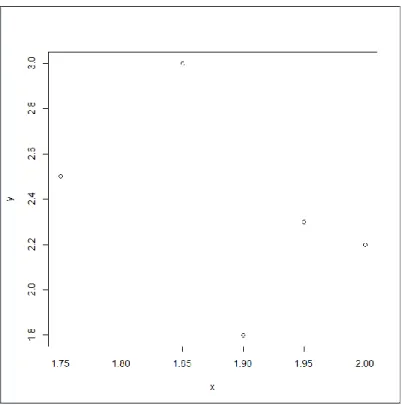
Table 2.1 List of the Data

Point X Y Point 1 1.75 2.5 Point 2 1.85 3.0 Point 3 1.90 1.8 Point 4 1.95 2.3 Point 5 2.00 2.2

(21)

Figure 1.1. Plot of the Data.

We now have to calculate the Euclidean distance between all of the pairs of points. The distance between the i-th and j-th point is calculated as follows:

Equation 2.1 Distance Function for Euclidean Distance

𝑑(𝑥_𝑖, 𝑥_𝑗) = √(𝑥_𝑖 − 𝑥_𝑗)2+ (𝑦_𝑖 − 𝑦_𝑗)2 _(2.1) For simplicity, this can be arranged into a matrix of distances between each pair of points.

(22)

Table 2.2

List of the Distance Matrix

Distance Point2 Point3 Point4 Point5

Point1 0.51 0.7159 0.2828 0.3905

Point2 1.201 0.7071 0.8139

Point3 0.5025 0.4123

Point4 0.4123

Looking at the distance matrix, we would combine clusters 4 and 5 together. Since we are using the single linkage from this point forward, we will use the minimum distance between the clusters if there is more than one point in a cluster (Gan, Ma, & Wu, 2007, p. 118). The

calculations are then made as follows: 𝐷({𝑃𝑜𝑖𝑛𝑡4, 𝑃𝑜𝑖𝑛𝑡5}, 𝑃𝑜𝑖𝑛𝑡1) = 𝑀𝑖𝑛({𝐷(𝑃𝑜𝑖𝑛𝑡4, 𝑃𝑜𝑖𝑛𝑡1)}, {𝐷(𝑃𝑜𝑖𝑛𝑡5, 𝑃𝑜𝑖𝑛𝑡1)}) = 𝑀𝑖𝑛(0.2828, 0.3905) = 0.2828 𝐷({𝑃𝑜𝑖𝑛𝑡4, 𝑃𝑜𝑖𝑛𝑡5}, 𝑃𝑜𝑖𝑛𝑡2) = 𝑀𝑖𝑛({𝐷(𝑃𝑜𝑖𝑛𝑡4, 𝑃𝑜𝑖𝑛𝑡2)}, {𝐷(𝑃𝑜𝑖𝑛𝑡5, 𝑃𝑜𝑖𝑛𝑡2)}) = 𝑀𝑖𝑛(0.7071, 0.8139) = 0.7071 𝐷({𝑃𝑜𝑖𝑛𝑡4, 𝑃𝑜𝑖𝑛𝑡5}, 𝑃𝑜𝑖𝑛𝑡3) = 𝑀𝑖𝑛({𝐷(𝑃𝑜𝑖𝑛𝑡4, 𝑃𝑜𝑖𝑛𝑡3)}, {𝐷(𝑃𝑜𝑖𝑛𝑡5, 𝑃𝑜𝑖𝑛𝑡3)})

(23)

= 𝑀𝑖𝑛(0.5025, 0.4123) = 0.4123

Table 2.3

Distance Matrix Single Combine Point {4,5}

Distance Point2 Point3 {Point4,Point5}

Point1 0.51 0.7159 0.2828

Point2 1.201 0.7071

Point3 0.4123

The two closest clusters are the Point 1 and {Point 4, Point 5}. We combine these two clusters into one cluster and recalculate the distance matrix.

𝐷({𝑃𝑜𝑖𝑛𝑡1, 𝑃𝑜𝑖𝑛𝑡4, 𝑃𝑜𝑖𝑛𝑡5}, 𝑃𝑜𝑖𝑛𝑡2) = 𝑀𝑖𝑛(𝐷({𝑃𝑜𝑖𝑛𝑡4, 𝑃𝑜𝑖𝑛𝑡5}, 𝑃𝑜𝑖𝑛𝑡2), 𝐷(𝑃𝑜𝑖𝑛𝑡1, 𝑃𝑜𝑖𝑛𝑡2)) = 𝑀𝑖𝑛(0.7071, 0.51) = 0.51 𝐷({𝑃𝑜𝑖𝑛𝑡1, 𝑃𝑜𝑖𝑛𝑡4, 𝑃𝑜𝑖𝑛𝑡5}, 𝑃𝑜𝑖𝑛𝑡3) = 𝑀𝑖𝑛(𝐷({𝑃𝑜𝑖𝑛𝑡4, 𝑃𝑜𝑖𝑛𝑡5}, 𝑃𝑜𝑖𝑛𝑡3), 𝐷(𝑃𝑜𝑖𝑛𝑡1, 𝑃𝑜𝑖𝑛𝑡3)) = 𝑀𝑖𝑛(0.4123, 0.7159) = 0.4123 Table 2.4

(24)

The smallest distance is 0.4123, so combining Point 3 with {Point 1, Point 4, Point 5} to form a cluster. We recalculate the distance matrix. There are only two clusters left we know that they will be combined in the last step. The calculation is as follows.

𝐷({𝑃𝑜𝑖𝑛𝑡1, 𝑃𝑜𝑖𝑛𝑡3, 𝑃𝑜𝑖𝑛𝑡4, 𝑃𝑜𝑖𝑛𝑡5}, 𝑃𝑜𝑖𝑛𝑡2)

= 𝑀𝑎𝑥(𝐷({𝑃𝑜𝑖𝑛𝑡1, 𝑃𝑜𝑖𝑛𝑡4, 𝑃𝑜𝑖𝑛𝑡5}, 𝑃𝑜𝑖𝑛𝑡2), 𝐷(𝑃𝑜𝑖𝑛𝑡3, 𝑃𝑜𝑖𝑛𝑡2)) = 𝑀𝑎𝑥(0.51, 1.201)

= 0.51

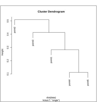
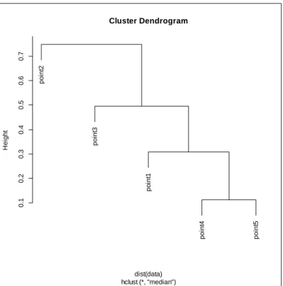
Figure 2.2. Dendrogram for the Single Linkage Method.

Looking at this figure, we can see that we first combined the points 4 and 5 into a cluster. Then as the height gets bigger we connect more points to the cluster.

p o in t2 p o in t3 p o in t1 p o in t4 p o in t5 0 .1 0 .2 0 .3 0 .4 0 .5 Cluster Dendrogram hclust (*, "single") dist(data) H e ig h t

(25)

2.2. Hierarchical Clustering with Average Linkage

The average linkage method is calculated by first taking the Euclidean distance of all pairs of data points. Merge the two points with the minimum distance. Next, take the average distance between each pair of clusters and merge the two clusters with the smallest average distance. This process is then repeated, until there is only one cluster.

Using the example data, we first combine points 1 and 5 since they are the closest. This then leads us to use the average distance when computing the next distance matrix. The distance between two points is then calculated as the average. Combining Point4 and Point5 since they are the smallest distance apart, we then have to calculate the distance from this cluster to the other points as follows:

𝐷({𝑃𝑜𝑖𝑛𝑡4, 𝑃𝑜𝑖𝑛𝑡5}, 𝑃𝑜𝑖𝑛𝑡1) = (1 2) ∗ (𝐷(𝑃𝑜𝑖𝑛𝑡4, 𝑃𝑜𝑖𝑛𝑡1) + 𝐷(𝑃𝑜𝑖𝑛𝑡5, 𝑃𝑜𝑖𝑛𝑡1)) = (1 2) ∗ (0.2828 + 0.3905) = 0.3367 𝐷({𝑃𝑜𝑖𝑛𝑡4, 𝑃𝑜𝑖𝑛𝑡5}, 𝑃𝑜𝑖𝑛𝑡2) = (1 2) ∗ 𝐷(𝑃𝑜𝑖𝑛𝑡4, 𝑃𝑜𝑖𝑛𝑡2) + ( 1 2) ∗ 𝐷(𝑃𝑜𝑖𝑛𝑡5, 𝑃𝑜𝑖𝑛𝑡2) = (1 2) ∗ 0.7071 + ( 1 2) ∗ 0.8139

(26)

𝐷({𝑃𝑜𝑖𝑛𝑡4, 𝑃𝑜𝑖𝑛𝑡5}, 𝑃𝑜𝑖𝑛𝑡3) = (1 2) ∗ 𝐷(𝑃𝑜𝑖𝑛𝑡4, 𝑃𝑜𝑖𝑛𝑡3) + ( 1 2) ∗ 𝐷(𝑃𝑜𝑖𝑛𝑡5, 𝑃𝑜𝑖𝑛𝑡3) = (1 2) ∗ 0.5025 + ( 1 2) ∗ 0.4123 = 0.4574 Table 2.5

Distance Matrix Average Combine Point {4,5}

Distance Point2 Point3 {Point4, Point5}

Point1 0.51 0.7159 0.3367

Point2 1.201 0.7605

Point3 0.4574

After combining Point 1 with Point 4 and 5, we then come up with a new distance matrix. The calculations for this matrix are as follows:

𝐷({𝑃𝑜𝑖𝑛𝑡1, 𝑃𝑜𝑖𝑛𝑡4, 𝑃𝑜𝑖𝑛𝑡5}, 𝑃𝑜𝑖𝑛𝑡2) = (1 3) ∗ (𝐷(𝑃𝑜𝑖𝑛𝑡1, 𝑃𝑜𝑖𝑛𝑡2) + 𝐷(𝑃𝑜𝑖𝑛𝑡4, 𝑃𝑜𝑖𝑛𝑡2) + 𝐷(𝑃𝑜𝑖𝑛𝑡5, 𝑃𝑜𝑖𝑛𝑡2)) = (1 3) ∗ (0.51 + 0.7071 + 0.8139) = 0.677

(27)

𝐷({𝑃𝑜𝑖𝑛𝑡1, 𝑃𝑜𝑖𝑛𝑡4, 𝑃𝑜𝑖𝑛𝑡5}, 𝑃𝑜𝑖𝑛𝑡3) = (1 3) ∗ (𝐷(𝑃𝑜𝑖𝑛𝑡1, 𝑃𝑜𝑖𝑛𝑡3) + 𝐷(𝑃𝑜𝑖𝑛𝑡4, 𝑃𝑜𝑖𝑛𝑡3) + 𝐷(𝑃𝑜𝑖𝑛𝑡5, 𝑃𝑜𝑖𝑛𝑡3)) = (1 3) ∗ (0.7159 + 0.5025 + 0.4123) = 0.5436 Table 2.6

Distance Matrix Average Combine Point {1,4,5}

Distance Point3 {Point1, Point4, Point5}

Point2 1.201 0.677

Point3 0.5436

After the calculation, combine Point 3 with Points 1, 4, 5. We have the following distance matrix: 𝐷({𝑃𝑜𝑖𝑛𝑡1, 𝑃𝑜𝑖𝑛𝑡3, 𝑃𝑜𝑖𝑛𝑡4, 𝑃𝑜𝑖𝑛𝑡5}, 𝑃𝑜𝑖𝑛𝑡2) = (1 4) ∗ (𝐷(𝑃𝑜𝑖𝑛𝑡1, 𝑃𝑜𝑖𝑛𝑡2) + 𝐷(𝑃𝑜𝑖𝑛𝑡3, 𝑃𝑜𝑖𝑛𝑡2) + 𝐷(𝑃𝑜𝑖𝑛𝑡4, 𝑃𝑜𝑖𝑛𝑡2) + 𝐷(𝑃𝑜𝑖𝑛𝑡5, 𝑃𝑜𝑖𝑛𝑡2)) = (1 4) ∗ (0.51 + 1.201 + 0.7071 + 0.8139) = 0.5436 Table 2.7

(28)

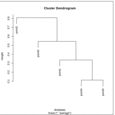
We are then left with combining Point 2 with the other points to form one large cluster (Gan, Ma, & Wu, 2007, p. 122).

Figure 2.3. Dendrogram for the Average Linkage Method.

The dendrogram summarizes the calculations of the points that join at different distances.

2.3. Hierarchical Clustering with Centroid Linkage

The centroid method is calculated by first taking the Euclidean distance of all the pairs of data. First, combine the two closest points to form a cluster.

Equation 2.2 Distance Function for the Centroid Method 𝐷(𝐶_𝑘 , 𝐶_𝑖 ∪ 𝐶_𝑗) = 𝑛𝑖 𝑛_𝑖 + 𝑛_𝑗𝐷(𝐶𝑘 , 𝐶𝑖) + 𝑛_𝑗 𝑛_𝑖 + 𝑛_𝑗𝐷(𝐶𝑘 , 𝐶𝑗) − 𝑛𝑖 (𝑛_𝑖 + 𝑛_𝑗)2𝐷(𝐶𝑖 , 𝐶𝑗) 𝑛𝑘 𝑖𝑠 𝑡ℎ𝑒 𝑛𝑢𝑚𝑏𝑒𝑟 𝑜𝑓 𝑒𝑙𝑒𝑚𝑒𝑛𝑡𝑠 𝑖𝑛 𝑐𝑙𝑢𝑠𝑡𝑒𝑟 𝑘 𝑛𝑗 𝑖𝑠 𝑡ℎ𝑒 𝑛𝑢𝑚𝑏𝑒𝑟 𝑜𝑓 𝑒𝑙𝑒𝑚𝑒𝑛𝑡𝑠 𝑖𝑛 𝑐𝑙𝑢𝑠𝑡𝑒𝑟 𝑗 𝑛_𝑖 𝑖𝑠 𝑡ℎ𝑒 𝑛𝑢𝑚𝑏𝑒𝑟 𝑜𝑓 𝑒𝑙𝑒𝑚𝑒𝑛𝑡𝑠 𝑖𝑛 𝑐𝑙𝑢𝑠𝑡𝑒𝑟 𝑖 (2.2) p o in t2 p o in t3 p o in t1 p o in t4 p o in t5 0 .1 0 .2 0 .3 0 .4 0 .5 0 .6 0 .7 0 .8 Cluster Dendrogram hclust (*, "average") dist(data) H e ig h t

(29)

Combine Point 4 and 5 since it is the smallest distance. The distance is then calculated as follows. 𝐷𝐷({𝑃𝑜𝑖𝑛𝑡4, 𝑃𝑜𝑖𝑛𝑡5 }, 𝑃𝑜𝑖𝑛𝑡1) = (1 2) ∗ (𝐷(𝑃𝑜𝑖𝑛𝑡4, 𝑃𝑜𝑖𝑛𝑡1) + 𝐷(𝑃𝑜𝑖𝑛𝑡5, 𝑃𝑜𝑖𝑛𝑡1)) − ( 1 4) ∗ 𝐷(𝑃𝑜𝑖𝑛𝑡4, 𝑃𝑜𝑖𝑛𝑡5) = (1 2) ∗ (0.2828 + 0.3905) − ( 1 4) ∗ 0.1118 = 0.3087 𝐷({𝑃𝑜𝑖𝑛𝑡4, 𝑃𝑜𝑖𝑛𝑡5 }, 𝑃𝑜𝑖𝑛𝑡2) = (1 2) ∗ (𝐷(𝑃𝑜𝑖𝑛𝑡4, 𝑃𝑜𝑖𝑛𝑡2) + 𝐷(𝑃𝑜𝑖𝑛𝑡5, 𝑃𝑜𝑖𝑛𝑡2)) − ( 1 4) ∗ 𝐷(𝑃𝑜𝑖𝑛𝑡4, 𝑃𝑜𝑖𝑛𝑡5) = (1 2) ∗ (0.7071 + 0.8139) − ( 1 4) ∗ 0.1118 = 0.7326 𝐷({𝑃𝑜𝑖𝑛𝑡4, 𝑃𝑜𝑖𝑛𝑡5 }, 𝑃𝑜𝑖𝑛𝑡3) = (1 2) ∗ (𝐷(𝑃𝑜𝑖𝑛𝑡4, 𝑃𝑜𝑖𝑛𝑡3) + 𝐷(𝑃𝑜𝑖𝑛𝑡5, 𝑃𝑜𝑖𝑛𝑡3)) − ( 1 4) ∗ 𝐷(𝑃𝑜𝑖𝑛𝑡4, 𝑃𝑜𝑖𝑛𝑡5) = (1) ∗ (0.5025 + 0.4123) − (1) ∗ 0.1118

(30)

Table 2.8

Distance Matrix Centroid Combine Point {4,5}

Point1 0.51 0.7159 0.3087

Point2 1.201 0.7326

Point3 0.4295

Combine the points with the smallest entry which is 0.3087. After combining Point1 with Point 4 and 5, we calculate the next distance matrix as follows.

𝐷({𝑃𝑜𝑖𝑛𝑡1, 𝑃𝑜𝑖𝑛𝑡4, 𝑃𝑜𝑖𝑛𝑡5 }, 𝑃𝑜𝑖𝑛𝑡2) = (2 3) ∗ 𝐷({𝑃𝑜𝑖𝑛𝑡4, 𝑃𝑜𝑖𝑛𝑡5}, 𝑃𝑜𝑖𝑛𝑡2) + (1 3) ∗ 𝐷(𝑃𝑜𝑖𝑛𝑡2, 𝑃𝑜𝑖𝑛𝑡1) − ( 2 9) ∗ 𝐷({𝑃𝑜𝑖𝑛𝑡4, 𝑃𝑜𝑖𝑛𝑡5}, 𝑃𝑜𝑖𝑛𝑡1) = (2 3) ∗ 0.7326 + ( 1 3) ∗ 0.51 − ( 2 9) ∗ 0.3087 = 0.5898 𝐷({𝑃𝑜𝑖𝑛𝑡1, 𝑃𝑜𝑖𝑛𝑡4, 𝑃𝑜𝑖𝑛𝑡5 }, 𝑃𝑜𝑖𝑛𝑡3) = (2 3) ∗ 𝐷({𝑃𝑜𝑖𝑛𝑡4, 𝑃𝑜𝑖𝑛𝑡5}, 𝑃𝑜𝑖𝑛𝑡3) + (1 3) ∗ 𝐷(𝑃𝑜𝑖𝑛𝑡3, 𝑃𝑜𝑖𝑛𝑡1) − ( 2 9) ∗ 𝐷({𝑃𝑜𝑖𝑛𝑡4, 𝑃𝑜𝑖𝑛𝑡5}, 𝑃𝑜𝑖𝑛𝑡1) = (2 3) ∗ 0.4295 + ( 1 3) ∗ 0.7159 − ( 2 9) ∗ 0.3087 = 0.4564

(31)

Table 2.9

Distance Matrix Centroid Combine Point {1,4,5}

Point2 1.201 0.5898

Point3 0.4564

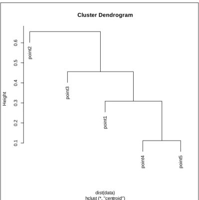
We combine {Point1, Point4, Point 5} with Point 3 since it has the minimum distance. We then obtain the next distance matrix. This is consequently the last calculation so it is known that these two clusters will be combined (Gan, 126). For illustration purposes the calculation is as follows. 𝐷({𝑃𝑜𝑖𝑛𝑡1, 𝑃𝑜𝑖𝑛𝑡3, 𝑃𝑜𝑖𝑛𝑡4, 𝑃𝑜𝑖𝑛𝑡5 }, 𝑃𝑜𝑖𝑛𝑡2) = (3 4) ∗ 𝐷({𝑃𝑜𝑖𝑛𝑡1, 𝑃𝑜𝑖𝑛𝑡4, 𝑃𝑜𝑖𝑛𝑡5}, 𝑃𝑜𝑖𝑛𝑡2) + (1 4) ∗ 𝐷(𝑃𝑜𝑖𝑛𝑡3, 𝑃𝑜𝑖𝑛𝑡2) − ( 3 16) ∗ 𝐷({𝑃𝑜𝑖𝑛𝑡1, 𝑃𝑜𝑖𝑛𝑡4, 𝑃𝑜𝑖𝑛𝑡5}, 𝑃𝑜𝑖𝑛𝑡3) = (3 4) ∗ 0.5898 + ( 1 4) ∗ 1.201 − ( 3 16) ∗ 0.4564 = 0.6570

(32)

Figure 2.4. Dendrogram for the Centroid Linkage Method.

2.4. Hierarchical Clustering with Complete Linkage

The complete linkage method is calculated first, by taking the Euclidean distance of all pairs of the data. First, pair the minimum two points to form a new cluster. Then, take the

maximum distance between each pair of points within the cluster we just combined. Next, merge the two points with the minimum distance. After you calculate the distance as the maximum distance between the clusters; combine the clusters with the smallest maximum distance. This process is repeated until there is only one cluster. This method is also known as the furthest neighbor; as it combines the two clusters with the closest maximum distance. Here is an example to help illustrate.

The closest distance is 0.118; we combine these two clusters. This leaves us with the following table. We must take the distance between all the points; while comparing with the max of the cluster we previously combined.

p o in t2 p o in t3 p o in t1 p o in t4 p o in t5 0 .1 0 .2 0 .3 0 .4 0 .5 0 .6 Cluster Dendrogram hclust (*, "centroid") dist(data) H e ig h t

(33)

𝐷({𝑃𝑜𝑖𝑛𝑡4, 𝑃𝑜𝑖𝑛𝑡5}, 𝑃𝑜𝑖𝑛𝑡1) = 𝑀𝑎𝑥({𝐷(𝑃𝑜𝑖𝑛𝑡4, 𝑃𝑜𝑖𝑛𝑡1)}, {𝐷(𝑃𝑜𝑖𝑛𝑡5, 𝑃𝑜𝑖𝑛𝑡1)}) = 𝑀𝑎𝑥(0.2828, 0.3905) = 0.3905 𝐷({𝑃𝑜𝑖𝑛𝑡4, 𝑃𝑜𝑖𝑛𝑡5}, 𝑃𝑜𝑖𝑛𝑡2) = 𝑀𝑎𝑥({𝐷(𝑃𝑜𝑖𝑛𝑡4, 𝑃𝑜𝑖𝑛𝑡2)}, {𝐷(𝑃𝑜𝑖𝑛𝑡5, 𝑃𝑜𝑖𝑛𝑡2)}) = 𝑀𝑎𝑥(0.7071, 0.8139) = 0.8139 𝐷({𝑃𝑜𝑖𝑛𝑡4, 𝑃𝑜𝑖𝑛𝑡5}, 𝑃𝑜𝑖𝑛𝑡3) = 𝑀𝑎𝑥({𝐷(𝑃𝑜𝑖𝑛𝑡4, 𝑃𝑜𝑖𝑛𝑡3)}, {𝐷(𝑃𝑜𝑖𝑛𝑡5, 𝑃𝑜𝑖𝑛𝑡3)}) = 𝑀𝑎𝑥(0.5025, 0.4123) = 0.5025 Table 2.10

Distance Matrix Complete Point {4,5}

Point1 0.51 0.7159 0.3905

Point2 1.201 0.8139

(34)

𝐷({𝑃𝑜𝑖𝑛𝑡1, 𝑃𝑜𝑖𝑛𝑡4, 𝑃𝑜𝑖𝑛𝑡5}, 𝑃𝑜𝑖𝑛𝑡2) = 𝑀𝑎𝑥(𝐷({𝑃𝑜𝑖𝑛𝑡4, 𝑃𝑜𝑖𝑛𝑡5}, 𝑃𝑜𝑖𝑛𝑡2), 𝐷(𝑃𝑜𝑖𝑛𝑡1, 𝑃𝑜𝑖𝑛𝑡2)) = 𝑀𝑎𝑥(0.8139, 0.51) = 0.8139 𝐷({𝑃𝑜𝑖𝑛𝑡1, 𝑃𝑜𝑖𝑛𝑡4, 𝑃𝑜𝑖𝑛𝑡5}, 𝑃𝑜𝑖𝑛𝑡3) = 𝑀𝑎𝑥(𝐷({𝑃𝑜𝑖𝑛𝑡4, 𝑃𝑜𝑖𝑛𝑡5}, 𝑃𝑜𝑖𝑛𝑡3), 𝐷(𝑃𝑜𝑖𝑛𝑡1, 𝑃𝑜𝑖𝑛𝑡3)) = 𝑀𝑎𝑥(0.5025, 0.7159) = 0.7159 Table 2.11

Distance Matrix Complete Point {1,4,5}

Point2 1.201 0.8139

Point3 0.7159

This means we would combine Point3 with {Point1, Point2, Point5}. This leads to the following distance matrix. There is only one way to merge these which leads to the completion of the method (Gan, 120).

= 𝑀𝑎𝑥(𝐷({𝑃𝑜𝑖𝑛𝑡1, 𝑃𝑜𝑖𝑛𝑡4, 𝑃𝑜𝑖𝑛𝑡5}, 𝑃𝑜𝑖𝑛𝑡2), 𝐷(𝑃𝑜𝑖𝑛𝑡3, 𝑃𝑜𝑖𝑛𝑡2)) = 𝑀𝑎𝑥(0.8139, 1.201)

(35)

Table 2.12

Distance Matrix Complete Point {1,3,4,5}

Distance {Point1,Point3, Point4, Point5}

Point2 1.201

Figure 2.5. Dendrogram for the Complete Linkage Method.

2.5. Hierarchical Clustering with Median Linkage

Median method uses a different distance function than the other methods. In each step the distance between the new cluster and the other clusters is calculated as follows (Gan, 130).

p o in t2 p o in t3 p o in t1 p o in t4 p o in t5 0 .0 0 .2 0 .4 0 .6 0 .8 1 .0 1 .2 Cluster Dendrogram hclust (*, "complete") dist(data) H e ig h t

(36)

𝐷({𝑃𝑜𝑖𝑛𝑡4, 𝑃𝑜𝑖𝑛𝑡5 }, 𝑃𝑜𝑖𝑛𝑡1) = (1 2) ∗ (𝐷(𝑃𝑜𝑖𝑛𝑡4, 𝑃𝑜𝑖𝑛𝑡1) + 𝐷(𝑃𝑜𝑖𝑛𝑡5, 𝑃𝑜𝑖𝑛𝑡1)) − ( 1 4) ∗ 𝐷(𝑃𝑜𝑖𝑛𝑡4, 𝑃𝑜𝑖𝑛𝑡5) = (1 2) ∗ (0.2828 + 0.3905) − ( 1 4) ∗ 0.1118 = 0.3087 𝐷({𝑃𝑜𝑖𝑛𝑡4, 𝑃𝑜𝑖𝑛𝑡5 }, 𝑃𝑜𝑖𝑛𝑡2) = (1 2) ∗ (𝐷(𝑃𝑜𝑖𝑛𝑡4, 𝑃𝑜𝑖𝑛𝑡2) + 𝐷(𝑃𝑜𝑖𝑛𝑡5, 𝑃𝑜𝑖𝑛𝑡2)) − ( 1 4) ∗ 𝐷(𝑃𝑜𝑖𝑛𝑡4, 𝑃𝑜𝑖𝑛𝑡5) = (1 2) ∗ (0.7071 + 0.8139) − ( 1 4) ∗ 0.1118 = 0.7326 𝐷({𝑃𝑜𝑖𝑛𝑡4, 𝑃𝑜𝑖𝑛𝑡5 }, 𝑃𝑜𝑖𝑛𝑡3) = (1 2) ∗ (𝐷(𝑃𝑜𝑖𝑛𝑡4, 𝑃𝑜𝑖𝑛𝑡3) + 𝐷(𝑃𝑜𝑖𝑛𝑡5, 𝑃𝑜𝑖𝑛𝑡3)) − ( 1 4) ∗ 𝐷(𝑃𝑜𝑖𝑛𝑡4, 𝑃𝑜𝑖𝑛𝑡5) = (1 2) ∗ (0.5025 + 0.4123) − ( 1 4) ∗ 0.1118 = 0.4295

(37)

Table 2.13

Distance Matrix Median Point {4,5}

Point1 0.51 0.7159 0.3087

Point2 1.201 0.7326

Point3 0.4295

Since 0.3087 is the smallest distance we combine {Point4, Point5} with Point1 to form a new cluster. We then can calculate the distances to this newly formed cluster {Point1, Point4, Point5}. 𝐷({𝑃𝑜𝑖𝑛𝑡1, 𝑃𝑜𝑖𝑛𝑡4, 𝑃𝑜𝑖𝑛𝑡5 }, 𝑃𝑜𝑖𝑛𝑡2) = (1 2) ∗ (𝐷({𝑃𝑜𝑖𝑛𝑡4, 𝑃𝑜𝑖𝑛𝑡5}, 𝑃𝑜𝑖𝑛𝑡2) + 𝐷(𝑃𝑜𝑖𝑛𝑡1, 𝑃𝑜𝑖𝑛𝑡2)) − (1 4) ∗ 𝐷({𝑃𝑜𝑖𝑛𝑡4, 𝑃𝑜𝑖𝑛𝑡5}, 𝑃𝑜𝑖𝑛𝑡1) = (1 2) ∗ (0.7326 + 0.51) − ( 1 4) ∗ 0.3087 = 0.5441 𝐷({𝑃𝑜𝑖𝑛𝑡1, 𝑃𝑜𝑖𝑛𝑡4, 𝑃𝑜𝑖𝑛𝑡5 }, 𝑃𝑜𝑖𝑛𝑡3) = (1 2) ∗ (𝐷({𝑃𝑜𝑖𝑛𝑡4, 𝑃𝑜𝑖𝑛𝑡5}, 𝑃𝑜𝑖𝑛𝑡3) + 𝐷(𝑃𝑜𝑖𝑛𝑡1, 𝑃𝑜𝑖𝑛𝑡3)) − (1 4) ∗ 𝐷({𝑃𝑜𝑖𝑛𝑡4, 𝑃𝑜𝑖𝑛𝑡5}, 𝑃𝑜𝑖𝑛𝑡3)

(38)

Table 2.14

Distance Matrix Median Point {1,4,5}

Point2 1.201 0.5441

Point3 0.4955

We combine {Point1,Point4,Point5} with Point3 to form a new cluster. Then we

calculate the distance from cluster {Point1, Point3, Point4, Point5} to the other points as follows: 𝐷({𝑃𝑜𝑖𝑛𝑡1, 𝑃𝑜𝑖𝑛𝑡3, 𝑃𝑜𝑖𝑛𝑡4, 𝑃𝑜𝑖𝑛𝑡5 }, 𝑃𝑜𝑖𝑛𝑡2) = (1 2) ∗ (𝐷({𝑃𝑜𝑖𝑛𝑡1, 𝑃𝑜𝑖𝑛𝑡4, 𝑃𝑜𝑖𝑛𝑡5}, 𝑃𝑜𝑖𝑛𝑡2) + 𝐷(𝑃𝑜𝑖𝑛𝑡3, 𝑃𝑜𝑖𝑛𝑡2)) − (1 4) ∗ 𝐷({𝑃𝑜𝑖𝑛𝑡1, 𝑃𝑜𝑖𝑛𝑡4, 𝑃𝑜𝑖𝑛𝑡5}, 𝑃𝑜𝑖𝑛𝑡3) = (1 2) ∗ (0.5441 + 1.201) − ( 1 4) ∗ 0.4955 = 0.7487

The calculations agree with the dendrogram plot showing the hierarchy of the merging clusters.

(39)

Figure 2.6. Dendrogram for the Median Linkage Method.

2.6. Hierarchical Clustering with McQuitty’s Linkage

McQuitty’s method is very similar to the average linkage with the exception that it doesn’t keep taking the average. It keeps taking the middle of the two clusters that you want to combine (1966).

Equation 2.4 Distance Function for the McQuitty’s Method 𝐷(𝐶𝑘 , 𝐶𝑖 ∪ 𝐶𝑗) =

1

2𝐷(𝐶𝑘 , 𝐶𝑖) + 1

2𝐷(𝐶𝑘 , 𝐶𝑖) (2.4)

First, we combine Point 4 and Point 5 into one cluster since they are the closest together. This then leads us to use the average distance when computing the next distance matrix. The

p o in t2 p o in t3 p o in t1 p o in t4 p o in t5 0 .1 0 .2 0 .3 0 .4 0 .5 0 .6 0 .7 Cluster Dendrogram hclust (*, "median") dist(data) H e ig h t

(40)

𝐷({𝑃𝑜𝑖𝑛𝑡4, 𝑃𝑜𝑖𝑛𝑡5}, 𝑃𝑜𝑖𝑛𝑡1) = (1 2) ∗ (𝐷(𝑃𝑜𝑖𝑛𝑡4, 𝑃𝑜𝑖𝑛𝑡1) + 𝐷(𝑃𝑜𝑖𝑛𝑡5, 𝑃𝑜𝑖𝑛𝑡1)) = (1 2) ∗ (0.2828 + 0.3905) = 0.3367 𝐷({𝑃𝑜𝑖𝑛𝑡4, 𝑃𝑜𝑖𝑛𝑡5}, 𝑃𝑜𝑖𝑛𝑡2) = (1 2) ∗ 𝐷(𝑃𝑜𝑖𝑛𝑡4, 𝑃𝑜𝑖𝑛𝑡2) + ( 1 2) ∗ 𝐷(𝑃𝑜𝑖𝑛𝑡5, 𝑃𝑜𝑖𝑛𝑡2) = (1 2) ∗ 0.7071 + ( 1 2) ∗ 0.8139 = 0.7605 𝐷({𝑃𝑜𝑖𝑛𝑡4, 𝑃𝑜𝑖𝑛𝑡5}, 𝑃𝑜𝑖𝑛𝑡3) = (1 2) ∗ 𝐷(𝑃𝑜𝑖𝑛𝑡4, 𝑃𝑜𝑖𝑛𝑡3) + ( 1 2) ∗ 𝐷(𝑃𝑜𝑖𝑛𝑡5, 𝑃𝑜𝑖𝑛𝑡3) = (1 2) ∗ 0.5025 + ( 1 2) ∗ 0.4123 = 0.4574 Table 2.15

Distance Matrix McQuitty’s Point {4,5}

Point1 0.51 0.7159 0.3367

Point2 1.201 0.7605

(41)

After then combining Point 1 with Points 4 and 5, we then come up with a new distance matrix.

The calculations for this matrix are as follows: 𝐷({𝑃𝑜𝑖𝑛𝑡1, 𝑃𝑜𝑖𝑛𝑡4, 𝑃𝑜𝑖𝑛𝑡5}, 𝑃𝑜𝑖𝑛𝑡2) = (1 2) ∗ (𝐷({𝑃𝑜𝑖𝑛𝑡4, 𝑃𝑜𝑖𝑛𝑡5}, 𝑃𝑜𝑖𝑛𝑡2) + 𝐷(𝑃𝑜𝑖𝑛𝑡1, 𝑃𝑜𝑖𝑛𝑡2)) = (1 2) ∗ (0.7605 + 0.51) = 0.6353 𝐷({𝑃𝑜𝑖𝑛𝑡1, 𝑃𝑜𝑖𝑛𝑡4, 𝑃𝑜𝑖𝑛𝑡5}, 𝑃𝑜𝑖𝑛𝑡3) = (1 2) ∗ (𝐷({𝑃𝑜𝑖𝑛𝑡4, 𝑃𝑜𝑖𝑛𝑡5}, 𝑃𝑜𝑖𝑛𝑡3) + 𝐷(𝑃𝑜𝑖𝑛𝑡1, 𝑃𝑜𝑖𝑛𝑡3)) = (1 2) ∗ (0.4574 + 0.7159) = 0.5867 Table 2.16

Distance Matrix McQuitty’s Point {1,4,5}

Point2 1.201 0.6353

Point3 0.5867

After the calculation combine Point 3 with Points 1, 4, 5. We have the following distance matrix:

(42)

= (1

2) ∗ (𝐷({𝑃𝑜𝑖𝑛𝑡1, 𝑃𝑜𝑖𝑛𝑡4, 𝑃𝑜𝑖𝑛𝑡5}, 𝑃𝑜𝑖𝑛𝑡2)

+ 𝐷(𝑃𝑜𝑖𝑛𝑡3, 𝑃𝑜𝑖𝑛𝑡2)) = (1

2) ∗ (0.6353 + 1.201) = 0.9182

This agrees with the dendrogram which shows a visual of how the clusters were combined.

Figure 2.7. Dendrogram for the McQuitty’s Linkage Method.

2.7. Hierarchical Clustering with Ward’s Linkage

Ward’s method is quite different from the other hierarchical clustering algorithms. As opposed to using a distance function and taking the smallest distance to combine into a new cluster, Ward’s method minimizes the error sum of squares for each step (Gan, 132). This creates

p o in t2 p o in t3 p o in t1 p o in t4 p o in t5 0 .0 0 .2 0 .4 0 .6 0 .8 Cluster Dendrogram hclust (*, "mcquitty") dist(data) H e ig h t

(43)

a method that “minimizes variance.” Using Ward’s method there are three important equations to consider.

The first important equation is the distance function to combine clusters. Equation 2.5 Distance Function for the Ward’s Method

𝐷(𝐶_𝑘 , 𝐶_𝑖 ∪ 𝐶_𝑗) = |𝐶𝑘| + |𝐶𝑖| |𝐶_𝑘| + |𝐶_𝑖| + |𝐶_𝑗|𝐷(𝐶𝑘 , 𝐶𝑖) + |𝐶_𝑘| + |𝐶_𝑗| |𝐶_𝑘| + |𝐶_𝑖| + |𝐶_𝑗|𝐷(𝐶𝑘 , 𝐶𝑗) − |𝐶𝑘| |𝐶𝑘| + |𝐶𝑖| + |𝐶𝑗| 𝐷(𝐶_𝑖 , 𝐶_𝑗) (2.5)

The other is the change in the error sum of squares. This first change in error sum of squares is to be calculated when there are no clusters, but just data points.

Equation 2.6 Change in Error Sum of Squares for Two Points ∆𝐸𝑆𝑆_{𝑖 𝑗} = 1

2𝐷(𝑃𝑜𝑖𝑛𝑡 𝑖, 𝑃𝑜𝑖𝑛𝑡 𝑗)

2

(2.6)

When there is at least one cluster, we change to the following equation for the change in error sum of squares:

Equation 2.7 Change in Error Sum of Squares for Two Clusters ∆𝐸𝑆𝑆𝑘(𝑖𝑗) =

1

(44)

𝐸𝑆𝑆₁ = 𝐸𝑆𝑆₀+ ∆𝐸𝑆𝑆_{4 5}= (1

2) 𝐷(𝑃𝑜𝑖𝑛𝑡 𝑖, 𝑃𝑜𝑖𝑛𝑡 𝑗)

2 _{= (}1

2) ∗ 0.1118 = 0.0559

We now have our first cluster, which consists of Point 4 and Point 5. We can now update the distance matrix.

𝐷({𝑃𝑜𝑖𝑛𝑡4, 𝑃𝑜𝑖𝑛𝑡5}, 𝑃𝑜𝑖𝑛𝑡1) = (2 3) ∗ (𝐷(𝑃𝑜𝑖𝑛𝑡4, 𝑃𝑜𝑖𝑛𝑡1) + 𝐷(𝑃𝑜𝑖𝑛𝑡5, 𝑃𝑜𝑖𝑛𝑡1)) − ( 1 3) ∗ 𝐷(𝑃𝑜𝑖𝑛𝑡4, 𝑃𝑜𝑖𝑛𝑡5) = (2 3) ∗ (0.08 + 0.1525) − ( 1 3) ∗ (0.0125) = 0.1508 𝐷({𝑃𝑜𝑖𝑛𝑡4, 𝑃𝑜𝑖𝑛𝑡5}, 𝑃𝑜𝑖𝑛𝑡2) = (2 3) ∗ (𝐷(𝑃𝑜𝑖𝑛𝑡4, 𝑃𝑜𝑖𝑛𝑡2) + 𝐷(𝑃𝑜𝑖𝑛𝑡5, 𝑃𝑜𝑖𝑛𝑡2)) − ( 1 3) ∗ 𝐷(𝑃𝑜𝑖𝑛𝑡4, 𝑃𝑜𝑖𝑛𝑡5) = (2 3) ∗ (0.5 + 0.6625) − ( 1 3) ∗ (0.0125) = 0.7708 𝐷({𝑃𝑜𝑖𝑛𝑡4, 𝑃𝑜𝑖𝑛𝑡5}, 𝑃𝑜𝑖𝑛𝑡3) = (2 3) ∗ (𝐷(𝑃𝑜𝑖𝑛𝑡4, 𝑃𝑜𝑖𝑛𝑡3) + 𝐷(𝑃𝑜𝑖𝑛𝑡5, 𝑃𝑜𝑖𝑛𝑡3)) − ( 1 3) ∗ 𝐷(𝑃𝑜𝑖𝑛𝑡4, 𝑃𝑜𝑖𝑛𝑡5) = (2 3) ∗ (0.2525 + 0.17) − ( 1 3) ∗ (0.0125) = 0.2775

(45)

Table 2.17

Distance Matrix Ward’s Point {4,5}

Point1 0.26 0.5125 0.1508

Point2 1.4425 0.7708

Point3 0.2775

The smallest value is between Point 1 and {Point 4, Point 5}. So, after combining into one new cluster, we have to recalculate the error sum of squares.

𝐸𝑆𝑆2 = 𝐸𝑆𝑆1+ ∆𝐸𝑆𝑆45 1 = 0.0559 + ( 1 2) ∗ 0.1508 = 0.1313 𝐷({𝑃𝑜𝑖𝑛𝑡1, 𝑃𝑜𝑖𝑛𝑡4, 𝑃𝑜𝑖𝑛𝑡5}, 𝑃𝑜𝑖𝑛𝑡2) = (2 4) ∗ 𝐷(𝑃𝑜𝑖𝑛𝑡1, 𝑃𝑜𝑖𝑛𝑡2) + ( 3 4) ∗ 𝐷({𝑃𝑜𝑖𝑛𝑡4, 𝑃𝑜𝑖𝑛𝑡5}, 𝑃𝑜𝑖𝑛𝑡2)) − (1 4) ∗ 𝐷({𝑃𝑜𝑖𝑛𝑡4, 𝑃𝑜𝑖𝑛𝑡 5}, 𝑃𝑜𝑖𝑛𝑡 1) = (2 4) ∗ 0.26 + ( 3 4) ∗ 0.7708 − ( 1 4) ∗ 0.1508 = 0.6704 𝐷({𝑃𝑜𝑖𝑛𝑡1, 𝑃𝑜𝑖𝑛𝑡4, 𝑃𝑜𝑖𝑛𝑡5}, 𝑃𝑜𝑖𝑛𝑡3) = (2 4) ∗ 𝐷(𝑃𝑜𝑖𝑛𝑡1, 𝑃𝑜𝑖𝑛𝑡3) + ( 3 4) ∗ 𝐷({𝑃𝑜𝑖𝑛𝑡4, 𝑃𝑜𝑖𝑛𝑡5}, 𝑃𝑜𝑖𝑛𝑡3))

(46)

Table 2.18

Distance Matrix Ward’s Point {1, 4,5}

Point2 1.4425 0.6704

Point3 0.4267

𝐸𝑆𝑆₃ = 𝐸𝑆𝑆₂+ ∆𝐸𝑆𝑆_{145 3}= 0.1313 + (1

2) ∗ 0.4267 = 0.3447

Then the distances must be recalculated. So, the main idea is to keep calculating the error sum of squares and combine the clusters that minimize the error sum of squares.

𝐷({𝑃𝑜𝑖𝑛𝑡1, 𝑃𝑜𝑖𝑛𝑡3, 𝑃𝑜𝑖𝑛𝑡4, 𝑃𝑜𝑖𝑛𝑡5}, 𝑃𝑜𝑖𝑛𝑡2) = (2 5) ∗ 𝐷(𝑃𝑜𝑖𝑛𝑡2, 𝑃𝑜𝑖𝑛𝑡3) + ( 4 5) ∗ 𝐷({𝑃𝑜𝑖𝑛𝑡1, 𝑃𝑜𝑖𝑛𝑡4, 𝑃𝑜𝑖𝑛𝑡5}, 𝑃𝑜𝑖𝑛𝑡2) − (1 5) ∗ 𝐷({𝑃𝑜𝑖𝑛𝑡1, 𝑃𝑜𝑖𝑛𝑡4, 𝑃𝑜𝑖𝑛𝑡 5}, 𝑃𝑜𝑖𝑛𝑡3) = (2 5) ∗ 1.4425 + ( 4 5) ∗ 0.6704 − ( 1 5) ∗ 0.4267 = 1.0280 Table 2.19

Distance Matrix Ward’s Point {1,3,4,5}

Distance {Point1, Point3, Point4, Point5}

Point2 1.0280

Then the entire cluster merging has been completed, but the last calculations are as follows.

(47)

𝐸𝑆𝑆₄ = 𝐸𝑆𝑆₃+ ∆𝐸𝑆𝑆_{1345 2}= 0.3447 + (1

2) ∗ 1.0280 = 0.8587

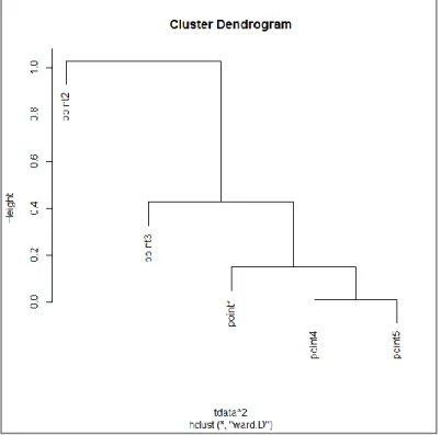
Figure 2.8. Dendrogram for the Ward’s Linkage Method.

The dendrogram agrees with the calculations.

2.8. K-means Clustering Algorithm

K-means is an iterative algorithm that needs the number of clusters specified in order to run. The main idea behind k-means is the initialization phase. For this phase you decide how many clusters you are trying to separate the data into. Let’s say you are trying to assign the data into k clusters. First, choose k points at random without replacement. Then the iteration phase

(48)

recommended to specify a maximum iteration. This will assure you will not be searching forever. Then you can just restart the initialization phase again and try again with k new points.

Applying this to the previous example, assume you are trying to cluster data into 2 clusters. K-means randomly chooses 2 different points. From these two points each other point is assigned to be in the cluster that is closest to the randomly chosen points. After each point has been assigned to a cluster the means are recalculated. The points are again assigned to the cluster with the closest point. For example, let’s choose 2 points at random from our example. Without loss of generality, we chose Point 1 and Point 3. We then choose these values as our clusters. At that point we assign every other point to the closest cluster. Point 2 will be assigned to cluster 1 which consists of Point 1. Point 4 will be assigned to cluster 1 since it is closer. Point 5 will be assigned to cluster 1. Cluster 1 consists of Point 1, Point 2, Point 4 and Point 5. The second cluster consists of just Point 3. The mean is then recalculated for each cluster. Adding up all the x values for cluster 1, we get 7.55. Dividing by 4, we get and average x of 1.8875. Adding up all the y values for cluster 1, we get 10. Dividing by 4, we get an average y value of 2.5. So, we now have centers of clusters at (1.8875, 2.5) and (1.9, 1.8). All of the points are assigned to cluster 1 and cluster 2 consists of its only point. This process can happen very quick or sometimes not at all (Gan, 162).

2.9. PAM Clustering Algorithm

PAM stands for Partition Around Medoids. The clustering algorithm is very similar to K-means. There is just a few slight differences. The process for PAM is to first choose k points at random. These k points are considered to be the medoid. For each medoid assign each data point to the closest medoid. For each cluster, calculate the total cost. The total cost is defined as the sum of all of the distances from the medoid for that particular cluster. Then calculate the cost of

(49)

swapping a medoid. This means the replacement one of your medoids with another point. The reasoning is that maybe another medoid will result in a lower total cost. This process of

assigning points to the medoid then calculating the cost of swapping is repeated until there is no change in the medoid (Kaufman, 68).

For example consider 2 clusters for the example data. If we again randomly chose two points and choose Point 4 and Point 5 for the medoid. From these two medoids, we need to calculate the cost (Euclidean distance). We then end up with two tables. Let’s assume cluster 1 is Point 4 and cluster 2 is Point 5

Table 2.20

Cost Matrix For PAM

Point Cost to Point 4 Cost to Point 5 Assign

Point 1 0.2828 0.3905 Cluster 1

Point 2 0.7071 0.8139 Cluster 1

Point 3 0.5025 0.4123 Cluster 2

Point 4 Medoid

Point 5 Medoid

From these two starting medoids, we will then assign {Point 1 and Point 2} to cluster 1. We will then assign {Point 3} to cluster 2. We then calculate the total cost. This is the sum of the distances for each point to the cluster medoid.

(50)

Table 2.21

Cost Matrix For Swapping Points PAM

Point Cost to Point 2 Cost to Point 5 Assign

Point 1 0.51 0.3905 Cluster 2 Point 2 Medoid Point 3 1.201 0.4123 Cluster 2 Point 4 0.7071 0.1118 Cluster 2 Point 5 Medoid 𝑐𝑙𝑢𝑠𝑡𝑒𝑟1 𝑡𝑜𝑡𝑎𝑙 𝑐𝑜𝑠𝑡 = 0 𝑐𝑙𝑢𝑠𝑡𝑒𝑟2 𝑡𝑜𝑡𝑎𝑙 𝑐𝑜𝑠𝑡 = 0.3905 + 0.4123 + 0.1118 = 0.9146 𝑡𝑜𝑡𝑎𝑙 𝑐𝑜𝑠𝑡 = 0 + 0.9146 = 0.9146

There was a significant improvement to the total cost by using Point 2 as opposed to Point 4. This process of swapping and then recalculating the cost is repeated until there is no more improvement.

Average pairwise overlap is used because it is a measure of the level of difficulty in separation between clusters. Clusters that have a significant level of overlap are going to be harder to distinguish. Overlap between two clusters is the sum of misclassification probabilities (Maitra, 354-376).

Some sort of measure needs to be used in order to compare the cluster’s performance in its ability to classify. The Rand Index is a measure of how well the clusters agree with each other. It is a measure of how well two different classifications agree or disagree with each other. One flaw about the Rand Index is that it does not take into consideration the number of clusters; therefore, the Adjusted Rand Index is a better measure for performance of classification.

(51)

The Rand Index can be calculated by first creating a table of the classification of clusters. Let X be a set of n data points {x1, x1, .. xn}. Consider two different clustering classifications of the data points with the number of clusters equal to C. Let V denote the first classification vector of the data points {V1, V2,..VC}. Let U denote the classification vector of the data points {U1, U2,..UC}. A table is created to reflect the number of agreements between the two different clustering classifications. The table would look similar to the following (Yeung).

Table 2.22

Classification Table for Clusters

V1 V2 … VC RowSum U1 𝑛₁₁ 𝑛₁₂ … 𝑛_1𝐶 𝑛_1. U2 𝑛₂₁ 𝑛₁₁ … 𝑛_2𝐶 𝑛_2. … … … … … UC 𝑛_𝐶1 𝑛_𝐶2 … 𝑛_𝐶𝐶 𝑛_𝐶. ColSum 𝑛_.1 𝑛_.2 … 𝑛_.𝐶 TotalSum = n 𝑛_𝑖𝑗 = 𝑡ℎ𝑒 𝑛𝑢𝑚𝑏𝑒𝑟 𝑜𝑓 𝑎𝑔𝑟𝑒𝑒𝑚𝑒𝑛𝑡𝑠 𝑏𝑒𝑡𝑤𝑒𝑒𝑛 𝑈𝑖 𝑎𝑛𝑑 𝑉𝑗 𝑛.𝑗 = ∑ 𝑛𝑖𝑗 𝐶 𝑖=1 𝑛_𝑖. = ∑ 𝑛_𝑖𝑗 𝐶 𝑗=1

(52)

Equation 2.8 Number of Agreements

𝑎 = ∑ (𝑛𝑖𝑗 2 )

𝑖𝑗 (2.8)

Equation 2.9 Number of Objects in the same cluster for U but not in the same class in V 𝑏 = ∑ (𝑛𝑖. 2) 𝑖 − ∑ (𝑛𝑖𝑗 2 ) 𝑖𝑗 (2.9)

Equation 2.10 Number of Objects in the same cluster for V but not in the same class in U 𝑐 = ∑ (𝑛.𝑗 2) 𝑗 − ∑ (𝑛𝑖𝑗 2 ) 𝑖𝑗 (2.10)

Equation 2.11 Number of Disagreements 𝑑 = (𝑛

2) − 𝑎 − 𝑏 − 𝑐 (2.11)

Equation 2.12 Formula for the Rand Index

𝑅𝐼 = 𝑎 + 𝑑

𝑎 + 𝑏 + 𝑐 + 𝑑 (2.12)

Equation 2.13 Formula for the Adjusted Rand Index

𝐴𝑅𝐼 = ∑ (𝑛𝑖𝑗 2 ) 𝑖𝑗 − ∑ (𝑛𝑖. 2) ∑ ( 𝑛.𝑗 2) 𝑗 𝑖 (𝑛₂) 1 2[∑ (𝑖 𝑛𝑖.2)+∑ (𝑗 𝑛.𝑗2)]− ∑ (𝑖𝑛𝑖.₂) ∑ (𝑗 𝑛.𝑗₂) (𝑛₂) (2.13)

The Adjusted Rand Index is a measure of how well the clustering classification is done. It is bounded above by 1, but has no lower bound for the index. The benefit of the Adjusted Rand Index over the Rand index is that it has an expected value of 0. The Rand Index has an expected

(53)

value of something greater than 0 and less than 1. It is a measure that is not constant. This is a big draw back when comparing clusters because you do not know how good the clustering algorithm is relative to chance.

(54)

CHAPTER 3. METHODOLOGY

The purpose of this study is to compare 10 different clustering algorithms. The clustering algorithms used were PAM, K-means, and hierarchical clustering algorithms. The hierarchical clustering link functions used were Wards, Single, Complete, Average, McQuitty, Median, and Centroid. With this study, we will be able to conclude the best and worst clustering algorithms. The complexity in the data is from the number of dimensions (2, 5, 10), number of clusters (4, 8, 16), pairwise average overlap between the clusters (0.001, 0.005, 0.01, 0.05, 0.1, 0.2), and the average number of points simulated from each cluster (10, 25, 100). From these data, it will be repeated 1000 times. We did not simulate more repetitions, due to time constraints.

The data factors important in a simulation study are the type of data and how the data were simulated. We used Clustering Algorithms’ Referee Package (CARP), which is a C-package that is quite easy to implement in Linux. The reasoning behind using CARP is that it is very efficient; the layout is very easy to use and understand. The idea is to simulate mixture distributions with a certain condition; then simulate data from the mixtures. After the data has been simulated, the clustering algorithms will be used on each specific data set. The clustering algorithm will tell which data points are in each cluster. Since it is known where each data point is simulated from; we can gauge the accuracy of the clustering algorithm. Next, a pairwise comparison will be implemented to see how the clustering algorithms perform amongst each other.

First, the mixtures must be simulated. This is one of the most important parts of a simulation study. It is important because if the data being simulated does not have a significant amount of meaning, the results will have little impact in their importance. Different clustering algorithms are known to perform better under different situations. There is no known guide of

(55)

when to use a particular clustering algorithm. Since Gaussian data is the most common; it would make sense to test different clustering algorithms using Gaussian data. While using a Gaussian mixture data with a pre-specified average pairwise overlap and number of dimensions, we simulate the mixtures. This is accomplished with the command:

./CARP –G4 –p2 -b0.05 -#1000

The –G in the command specifies the number of mixing components. This command simulates a mixture with 4 mixing components. The –p in the command specifies the number of dimensions. This command specifies a 2 dimensional space. The –b in the command is the pairwise average overlap. The -# section of the command specifies how many mixtures you want. In this case, we would like 1000 different mixture distributions with a pairwise overlap of 0.05, the number of dimensions equal to 2, and the number of mixing components equal to 4.

From this mixture, we can simulate data from the Gaussian mixtures. In order to make the problem a little more complex, we will simulate a small (approximately 10 points), medium (approximately 25), and large (approximately 100 points) number of points from each cluster. Since this is simulated, the mixing proportions will be used as weights for the number of points simulated. For example, consider a mixture which has the mixing proportions of (1/4, 3/4), the majority of the mixture is composed from the second component. We would like most of the points to come from the second component of the mixture. One way to accomplish this is to set this up a Bernoulli with a proportion of success equal to 1/4. The randomness of which mixing

(56)

The only difference is now we do not have to specify the average overlap like we did in the previous command. Instead, we specify the average number of data points simulated from each mixture. From this statement, we get 1000 data sets composed of 2 dimensional Gaussian data with 4 mixing components with approximately 40 points from each mixing component.

Now that the data is simulated, we can run each of the clustering algorithms on the dataset. This is accomplished with the command:

./CARP -G4 -p2 -#1000 -n-40 -Rhierclust1.dat -Ahierclust1

The – between the n and the 40 represents data that have already been simulated. This indicates there is already 40 data points simulated and not to simulate new data. The –R is to output the Adjusted Rand Index. We specify this because we can then run each different clustering algorithm on the same set of data and output only the adjusted rand. The –A part of this command specifies which clustering algorithm is used. After repeating this for each different clustering algorithm, we can compare Adjusted Rand indices from each clustering method. Comparison is done using a two sample t-test.

In R: t.test(Hierclust1, Hierclust2)

Where Hierclust1 and Hierclust2 are the Adjusted Rand indices from the clustering algorithms used.

From the Adjusted Rands, we can figure the mean to determine the best to worst performing clustering algorithm. We then created a matrix of p values from the pairwise comparisons. One example of this would be:

(57)

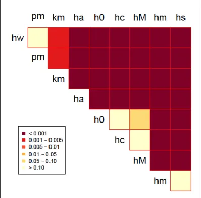
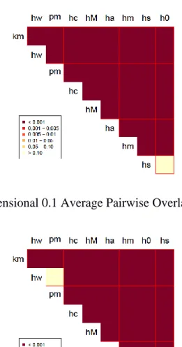
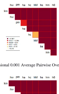
Figure 3.1. Four Cluster 2 Dimension 0.001 Average Pairwise Overlap with 40 Points.

As you can see, this is made into a format that is easy to understand. Each of the two letters would be the specific clustering algorithm. The heat map shows the p value. If the color is white or cream, there is no significant difference between the two clustering algorithms.

Whereas, if the color is not cream there is a significant difference between the two clustering algorithms. This heat map is then repeated for all the different combinations of dimensions, clusters, average pairwise overlap, and average number of elements in each cluster.

(58)

CHAPTER 4. RESULTS 4.1. Four Cluster Results

The results are quite interesting (see Appendix A). As you move from very little pairwise overlap to substantial pairwise overlap, you would think that the best clustering algorithm may differ. Looking at the results, it is the same three clustering algorithms that perform as the top three for all of the 4 cluster results. Dimensions had no effect on change the results of the best three clustering algorithms. An interesting result happens when considering the 2 dimensional space (Appendix A, Figures A.1-A.18). The clustering algorithm PAM (Partitioning Around Medoids) performs the best for most cases. There is one case when a hierarchical with Ward’s linkage performs significantly better than PAM (see Figure A.3).

(59)

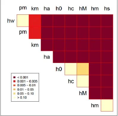
Figure 4.1 is an example of how every specific case of number of clusters, dimension, average pairwise overlap, and number of points simulated have been summarized. There are nine different abbreviations for the clustering algorithms which are illustrated in Table 4.1.

Table 4.1

Abbreviations of the Clustering Algorithms

Abbreviation Clustering Algorithm

hw Hierarchical with Ward’s linkage

hs Hierarchical with Single linkage

hc Hierarchical with Complete linkage

ha Hierarchical with Average linkage

hM Hierarchical with Mc Quitty’s linkage

hm Hierarchical with Median linkage

h0 Hierarchical with Centroid linkage

pm Partition Around Medoids (PAM)

km K-means

The clustering algorithms are sorted by the mean. Taking the average of all of the

adjusted Rand values for each different clustering algorithm, we can tell which performs the best. In order to do a comparison to see which clustering algorithms are statistically significant, a t-test will show a pairwise comparison of two clustering algorithms. T-tests are then repeated for all pairwise comparisons for each specific cluster, dimension, pairwise overlap, and number of

(60)

there is no significant difference between the two algorithms being compared for that particular square. If the color is slightly darker than cream it represents a p value inside the interval (0.05, 0.10). This would mean the two algorithms are not considered to be significantly different at an alpha level of 0.05. If the color has any shade of red, it represents a p value of less than 0.05. This would indicate that the two clustering algorithms are significantly different. The darker the shade of red, the more significant the p value would be.

One clustering algorithm that tied with PAM would be hierarchical with Ward’s linkage. This happened in 5 of the 18 cases, which mostly occurred when the average pairwise overlap was small (less than 0.005). The other clustering algorithm that tied with PAM was K-means. This algorithm tied in 3 of the 18 cases. This also happened when the average pairwise overlap was large (0.05, 0.1, 0.2) and when there was only a total of 40 points simulated. It was also interesting that it did not typically matter how many points were simulated from each cluster. One might think that if you have more points from each cluster that the results may differ; this was not true in the 4 cluster results.

While increasing the dimensions to 5 and 10 a new clustering algorithm emerged as the best performer; K-means performed the best for the majority of the dimensions equal to 5. There was one case (see Figure A.21) in which a hierarchical with Ward’s linkage performed the best. For all other cases, K-means was the best or not significantly different from the best performing clustering algorithm. The results for the 5 dimensional space can be found in Appendix A, Figures A.19-A.36. When the dimensions were increased to 10, the results did not change much from the 5 dimension space. In the 10 dimension space, K-means performed the best in all 18 cases (Figures A.37-A.54).

(61)

4.2. Eight Cluster Results

When the dimension fixed at 2, PAM performs the best for all cases. The results for the 8 cluster 2 dimension space can be found in Appendix B, Figures B.1-B.18. There are seven cases where three different algorithms performed with no significant difference than PAM. The other three algorithms are K-means, hierarchical with Ward’s linkage, and hierarchical with Average linkage. When the average pairwise overlap is 0.001 hierarchical with Ward’s linkage the

calculation performed the same as PAM for the number of points simulated equal to 200 and 800 (Figures B.2-B.3). When the average pairwise overlap was 0.01 Ward’s linkage also tied with PAM though this was only in the case where the number of points simulated was 80 (Figure B.7). There were two cases where all three (PAM, K-means, and hierarchical with Ward’s linkage) algorithms performed similarly to each other. These cases occurred when the number of points simulated was 80 and the average pairwise overlap was 0.05 and 0.1 (Figures B.10 and Figure B.13). This outcome was kind of a surprise since one would expect that when the average pairwise overlap is low, all the clustering algorithms would perform well. The powers of all the algorithms are high, but these three algorithms have the highest average adjusted Rand values.

When the average pairwise overlap was 0.2 and the number of points simulated equal to 80 and 200, K-means performs similarly to PAM (Figures B.16-B.17). When considering the number of dimensions equal to 5 (Figures B.19-B.36) and 10 (Figures B.37-B.54), K-means generally performed the best. There are three cases when K-means is outperformed by another