lCARE – localizing Conditional AutoRegressive Expectiles

SFB 649 Discussion Paper 2015-052

lCARE

–

localizing Conditional

AutoRegressive Expectiles

Xiu Xu*

Andrija Mihoci*²

Wolfgang Karl Härdle*³

* Humboldt-Universität zu Berlin, Germany *² Brandenburg University of Technology, Germany

*³ Humboldt-Universität zu Berlin, Germany ; and Singapore Management University, Singapore This research was supported by the Deutsche

Forschungsgemeinschaft through the SFB 649 "Economic Risk". http://sfb649.wiwi.hu-berlin.de

ISSN 1860-5664

SFB 649, Humboldt-Universität zu Berlin Spandauer Straße 1, D-10178 Berlin

SFB

6

4

9

E

C

O

N

O

M

I

C

R

I

S

K

B

E

R

L

I

N

lCARE - localizing Conditional AutoRegressive

Expectiles

∗

Xiu Xu

, Andrija Mihoci

, Wolfgang Karl Härdle

Abstract

We account for time-varying parameters in the conditional expectile based value at

risk (EVaR) model. EVaR appears more sensitive to the magnitude of portfolio losses

compared to the quantile-based Value at Risk (QVaR), nevertheless, by fitting the models

over relatively long ad-hoc fixed time intervals, research ignores the potential time-varying

parameter properties. Our work focuses on this issue by exploiting the local parametric

approach in quantifying tail risk dynamics. By achieving a balance between parameter

variability and modelling bias, one can safely fit a parametric expectile model over a stable

interval of homogeneity. Empirical evidence at three stock markets from 2005- 2014 shows that the parameter homogeneity interval lengths account for approximately 1-6 months of

daily observations. Our method outperforms models with one-year fixed intervals, as well

as quantile based candidates while employing a time invariant portfolio protection (TIPP)

strategy for the DAX portfolio. The tail risk measure implied by our model finally provides

valuable insights for asset allocation and portfolio insurance.

JEL classification: C32, C51, G17

Keywords: expectiles, tail risk, local parametric approach, risk management

∗_{Financial support from the Deutsche Forschungsgemeinschaft via CRC 649 ”Economic Risk” and}

IRTG 1792 ”High Dimensional Non Stationary Time Series”, Humboldt-Universität zu Berlin, is grate-fully acknowledged.

†_{Humboldt-Universität zu Berlin, C.A.S.E. - Center for Applied Statistics and Economics, Spandauer}

Str. 1, 10178 Berlin, Germany, tel: +49 (0)30 2093 5721, fax: +49 (0)30 2093 5649, Xiamen University, Wang Yanan Institute for Studies in Economics (WISE), 361005 Xiamen, China

‡_{Brandenburg University of Technology, Chair of Econometrics and Business Statistics, Erich Weinert}

Str. 1, 03046 Cottbus, Germany, tel: +49 (0)355 69 38 20

§_{Humboldt-Universität zu Berlin, C.A.S.E. - Center for Applied Statistics and Economics, Spandauer}

1

Introduction

Value at risk (VaR) is commonly used to measure the downside risk in finance, especially in portfolio risk management. Given a predetermined probability level, VaR evaluates the potential maximum loss for the targeted portfolio value; statistically it represents the quantile of the portfolio loss distribution, see Jorion (2000). Although it is straightforward to understand the VaR concept, it has been recently criticized. VaR lacks the property of sub-additivity, that is, under the VaR risk measure, the risk of a diversified portfolio is larger than the sum of each individual asset risk, which in turn contradicts the common wisdom of diversification. In light of this, Artzner et al. (1999) proposed the expected shortfall (ES) to measure portfolio risk, i.e., the expected loss below a given threshold (e.g., VaR) given the risk probability level.

Another undesirable aspect of the VaR measure is its insensitivity to the magnitude of the portfolio loss. Kuan et al. (2009) provide an example where, under a given probability level, the potential downside risk changes under different tail loss distributions while the corresponding VaR remains the same. Since VaR merely depends on the probability value and neglects the size of the downside loss, Kuan et al. (2009) proposed a downside risk measure, the expectile-based Value at Risk (EVaR), a more sensitive measure of the magnitude of extreme losses than the conventional quantile-based VaR (QVaR). The expectile at given level is estimated by minimizing the asymmetric weighted least squared errors, exploring the method proposed by Newey and Powell (1987). The expectile level is the relative cost of the expected margin shortfall, explained as the level of prudentiality. EVaR may be interpreted as a flexible QVaR (Kuan et al., 2009), because of the one-to-one mapping between quantiles and expectiles for a given loss distribution, see Efron (1991), Jones (1994) and Yao and Tong (1996).

Models based on the expectile risk measure framework have thus been proposed, see e.g. Taylor (2008) and Kuan et al. (2009) after Engle and Manganelli (2004) successfully initialize the conditional autoregressive framework to model VaR. Kuan et al. (2009) moreover extend the EVaR to conditional EVaR and propose various Conditional Au-toRegressive Expectile (CARE) specifications as well as establishing the asymptotic re-sults of Newey and Powell (1987) to allow for stationary and weakly dependent data.

Potential time-varying parameters resulting from the dynamic state of the economic and financial environment are however barely analysed. This is where this research comes into play. We focus on incorporating and reacting to potential structural breaks in order to estimate the tail risk measure.

The proposed local parametric approach (LPA) targets a parametric stable model in an adaptively chosen interval. The essential idea of the LPA is to find the longest inter-val length guaranteeing a relatively small modelling bias, see e.g. Spokoiny (1998) and Spokoiny (2009). The main advantage of the approach is the achievement of a balance between modelling bias and parameter variability. This approach has been successfully applied in many research areas: Čížek et al. (2009) analyse the GARCH(1,1) models, Chen et al. (2010) explore it to forecast realised volatilities, Chen and Niu (2014) predict the interest rate term structure, whereas Härdle et al. (2015) utilise it successfully in high frequency time series modelling and forecasting.

In this paper, we locally estimate the expectile risk measure rather than following a tradi-tional approach of assuming constant CARE parameters. Based on one of the conditradi-tional expectile model specifications in Kuan et al. (2009) and assuming that the error term follows the asymmetric normal distribution, Gerlach et al. (2012) and Gerlach and Chen (2014), we dynamically estimate the time-varying CARE parameters over potentially varying intervals of homogeneity. The desired interval of homogeneity is found by mul-tiple testing the null hypothesis that the model parameters are constant. The resulting time-varying interval lengths indicate potential structural changes in tail risk assessment. It is worth mentioning that several articles consider the dynamic window selection of time-varying parameters, Pesaran and Timmermann (2007) and Inoue et al. (2014), or introduce varying-coefficient models for tail risk measure estimation, Honda (2004), Kim (2007) and Cai and Xu (2008). Most of the research however mainly explores non-parametric approaches or considers polynomial splines to estimate the conditional quan-tile. A state space signal extraction algorithm to iteratively formulate quantile and non-parametrically obtain the quantile and expectile has been applied by De Rossi and Harvey (2009), whereas Xie et al. (2014) develop a nonparametric varying-coefficient approach to model the expectile-based value at risk.

In our research it turns out that the proposed localised conditional autoregressive expec-tile (lCARE) model successfully captures tail risk dynamics by taking the time-varying parameter characteristics and potential market condition structure changes into account while measuring the risk associated with tail events. Based on empirical results, we find that at the 5% expectile level the typical interval lengths that strike a balance between bias and variability in daily time series include approximately 100 days. At the lower, 1% expectile level, the selected interval lengths range roughly between 40-60 days. The resulting time-varying expectile series allows us to consider the dynamics of other tail risk measures, most prominently quantiles or expected shortfall.

The methodology presented here is successfully applied to a portfolio insurance strategy for the DAX index portfolio. A portfolio insurance strategy is designed to guarantee a minimum value for the asset portfolio over a selected investment horizon, where the downside risk can be reduced and controlled while investors can participate in the po-tential gains. The proportion of the value invested into the risky asset (here the DAX portfolio), denoted as the multiplier, is directly related to the estimated tail risk mea-sure. A standard approach keeps the multiplier fixed regardless of the market conditions, Estep and Kritzman (1988), Hamidi et al. (2014), whereas we exercise the protection strategy with the dynamic tail risk measure implied by the lCARE model. Comparison to the benchmarks - one-year fixed rolling window CARE estimation and quantile-based (CAViaR) estimation - reveals that the lCARE model presents a striking outperformance in portfolio insurance.

This paper is structured as follows: firstly, the data is presented in section 2 whereas section 3 introduces the lCARE model based on the CARE model setup and the local parametric approach in the tail risk modelling. Section 4 presents the empirical results and finally, section 5 concludes.

2

Data

In risk modelling we consider three stock markets and focus on the dynamics of the representative index time series, namely, DAX30, FTSE100 and S&P500 series. Daily

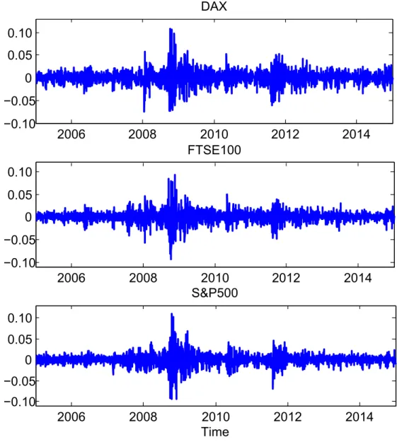
2006 2008 2010 2012 2014 −0.10 −0.05 0 0.05 0.10 DAX 2006 2008 2010 2012 2014 −0.10 −0.05 0 0.05 0.10 FTSE100 2006 2008 2010 2012 2014 −0.10 −0.05 0 0.05 0.10 S&P500 Time

Figure 1: Selected index return time series from 3 January 2005 to 31 December 2014

(2608 trading days). LCARE_Index_Returns

index returns are obtained from Datastream and our data cover the period from 3 Jan-uary 2005 to 31 December 2014, in total 2608 trading days. The daily returns evolve similarly across the selected markets and all present relatively large variations during the financial crisis period from 2008-2010, see, e.g., Figure 1. Although the return time series are nearly zero-mean with slightly pronounced skewness values, all present com-paratively high kurtosis, see, e.g., Table 1 that collects the summary statistics. Not-ing that the results and the correspondNot-ing Matlab codes can be found in the folder at https://github.com/QuantLet/lCARE-BTU-HUB and http://quantlet.de/d3/ia/.

Index Mean Median Min Max Std Skew. Kurt. DAX 0.0003 0.0007 -0.0743 0.1080 0.0137 0.0357 10.1654 FTSE100 0.0001 0.0001 -0.0927 0.0938 0.0120 -0.1498 11.9066 S&P500 0.0002 0.0005 -0.0947 0.1096 0.0127 -0.3364 14.5131

Table 1: Descriptive statistics for the selected index return time series from 3 Jan-uary 2005 to 31 December 2014 (2608 trading days): mean, median, minimum (Min), maximum (Max), standard deviation (Std), skewness (Skew.) and kurtosis (Kurt.). LCARE_Index_Returns_Description

3

Localized Conditional Autoregressive Expectiles

Understanding tail risk plays an essential role in asset pricing, portfolio allocation, invest-ment performance evaluation and external regulation. Tail event dynamics is commonly assessed through the employment of parametric, semi-parametric or nonparametric tech-niques, see, e.g., Taylor (2008). Our paper contributes to the econometric literature by localizing parametric CARE specifications by Kuan et al. (2009) and, while modelling tail risk, explores the effects of potential market structure changes. In this section we sum-marise the current research on expectile-based risk management and conduct a detailed empirical study concerning the parameter dynamics. The results motivate the usage of the local parametric approach by Spokoiny (1998) that is presented at the end of the chapter. The localized Conditional Autoregressive Expectiles (lCARE) model provides a statistical and applicable framework to analyse the downside risk in quantitative finance.

3.1

Conditional Autoregressive Expectile Model

Tail risk exposure can successfully be captured by an expectile-based risk measure, in contrast to modelling risk solely using Value at Risk (VaR). Despite being the most com-monly used (not coherent) tail risk measure, VaR exhibits insensitivity to the potential magnitude of the loss, see, e.g., Acerbi and Tasche (2002), Taylor (2008). After the condi-tional autoregressive value at risk (CAViaR) model by Engle and Manganelli (2004) was proposed, Taylor (2008) found that VaR, based on the conditional autoregressive expectile model, is more sensitive to the tail risk distribution. Finally, the conditional autoregres-sive expectile (CARE) model specifications by Kuan et al. (2009) directly model the

return time series and extend the asymmetric least square estimation method by Newey and Powell (1987) to analyse stationary but weakly dependent time series data.

The CARE model specifications provide insights into the dynamics of financial data and offer valuable economic interpretation. Although quantiles and expectiles belong to M-quantiles, see, e.g., Jones (1994), the implications in risk assessment differ considerably. VaR is a zero-moment whereas expectile is a first-moment tail risk measure, thus in the former case the proportion of asymmetric downside and upside quantile level is deter-mined only by the ratio between downside and upside probabilities. Expectiles measure the proportion of asymmetric downside and upside expectile level while capturing the ratio between the expected marginal shortfall. Equivalently, the potential cost of more extreme losses and the opportunity cost due to the expected marginal overcharge is cap-tured by expectiles. The CARE specifications furthermore accommodate stylised facts of the return time series, such as weak serial dependence, or volatility heteroskedasticity. Accommodating asymmetric effects on the tail expectiles of the positive and negative returns becomes essential in interpreting tail risk dynamics.

Based on the dynamics of an observed return time series y={yt}n_t=1, the CARE

frame-work is introduced as yt=et,τ +εt,τ (1) et,τ =α0,τ +α1,τyt−1+α2,τ y_t+₋₁2+α3,τ y_t−₋₁2 (2) where et,τ and εt,τ denote the expectile and the error term at level τ ∈ (0,1) and time

t, respectively. y+_t−1 = max{yt−1,0} and yt−−1 = min{yt−1,0} denote the positive or

negative observed one-period lagged returns, respectively.

Generally, the τ-level expectile et,τ in Equation (2) can be estimated by minimising the

asymmetric least square (ALS) loss function

n

X

t=2

|τ−I(yt≤et,τ)|(yt−et,τ)2 (3)

with I(·) denoting the indicator function.

that the error term εt,τ follows the asymmetric normal distribution (AND). We assume

that, conditional on the information set Ft−1, the data process follows an asymmetric

normal distribution ANDµ, σ2

ετ, τ with pdf: f(yt−µ| Ft−1) = 2 σετ s π |τ −1|+ r_π τ !−1 exp ( −ητ yt−µ σετ !) (4)

whereητ(u) =|τ −I{u≤0}|u2 is the employed check function, µrepresents the

expec-tile value to be estimated andσ2

ετ denotes the variance of the error term. Maximising the likelihood equation with respect toµfor the distribution (4) is asymptotically equivalent to minimising the asymmetric least square loss function (3).

Conditional on the information set Ft−1 up to observation (t−1), the expectile et,τ

includes a lagged return component and it mimics several financial series features, namely, the volatility clustering and potential asymmetric magnitude effects. Note that at level

τ = 0.5, the expectile equals to the mean value. With specification (3), the parameter vector finally contains five elements, namely θτ =

α0,τ, α1,τ, α2,τ, α3,τ, σ2ετ

>

.

In the specification (2), the parameterα1,τ indirectly measures the persistence level in the

conditional expectile tail through the lagged return series. Since the parameters α2,τ and

α3,τ potentially differ, (2) accounts for the asymmetric effects of the positive and negative

lagged squared returns on the conditional tail expectile magnitude. This similarly mimics the leverage effect associated with volatility modelling, where negative (positive) returns are followed by relatively larger (lower) variability. Under the working assumption that the expectile tail dynamics can be well approximated over a given data interval by a model with constant parameters, it suffices to include one-lag process dynamics.

The resulting quasi log likelihood function for observed dataY ={y1, . . . , yn}over a fixed

intervalI is given by

`I(Y;θτ) =

X

t∈I

logf(yt−et,τ | Ft−1) (5)

The quasi maximum likelihood estimate (QMLE) for the CARE parameter is then ob-tained through

e

θI,τ = arg max θτ∈Θ

over a right-end fixed interval I = [t0−m, t0] of (m+ 1) observations at observation t0.

3.2

Parameter Dynamics

The idea behind the local parametric approach (LPA) is to find the optimal (in-sample) data interval over which one can safely fit a parametric model with time-invariant pa-rameters. This optimal interval, the so-called interval of homogeneity, is selected among pre-specified right-end interval candidates. Over the resulting optimal data interval the proposed lCARE model allows the structure break properties of the expectile dynamics to be captured and therefore it can be used for expectile estimation. In this part we implement a fixed rolling window exercise in order to provide empirical evidence on the time-varying characteristics of the CARE estimates, as well as to select the ’true’ pa-rameter constellation used in the LPA simulation. At the end we discuss the estimation quality of the QMLE (6).

Dynamics and Distributional Characteristics

In the analysis of the selected (daily) stock market indices presented in Section 2, we consider different interval lengths (e.g., 20, 60, 125 and 250 observations) and provide the corresponding estimates. Shorter intervals will, in practice, result in larger variation as compared to longer ones, whereas the modelling bias behaves in the opposite direction: it is quite enlarged in the latter case. The distributional features of CARE parameters are moreover studied through two expectile level cases, namely τ = 0.05 and τ = 0.01. The following rolling window estimation exercise provides valuable insights into the expectile (distribution) dynamics.

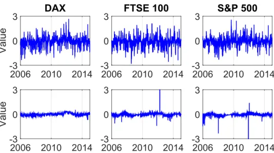
Parameter estimates are more volatile while fitting the data over shorter intervals with the modelling bias comparatively smaller as compared to schemes using longer intervals, see, e.g., Figures 2 and 3. Both figures namely present the estimated parameters αe1,0.05

and αe1,0.01 in the rolling window exercise across the three selected stock market indices

from 2 January 2006 to 31 December 2014 at fixed expectile levelsτ = 0.05 andτ = 0.01. The upper panel shows the estimation results with 20 observations and the lower panel with 250 observations.

The above mentioned properties are furthermore supported by the density estimates of the parameters involved, i.e., parameters belonging to the three stock market indices. Kernel density plots (using, e.g., a Gaussian kernel with optimal bandwidth) of estimated parameters show that shorter intervals lead to more variability and vice versa. For the sake of brevity, here we refrain from showing the density estimates. It is further verified that with fewer observations, such as including one month data (20 observations), the parameter density is distinguished from the estimates based on longer sample intervals, such as one year of data.

2006 2010 2014

Value

DAX

Value

FTSE 100

S&P 500

Figure 2: Estimated parameter αe1,0.05 across the three selected stock markets from

2 January 2006 to 31 December 2014, with 20 (upper panel) and 250 (lower panel) observations used in the rolling window exercise at fixed expectile level τ = 0.05. LCARE_Estimation_Rolling_005

Descriptive Statistics

The lCARE testing framework demands a set of simulated critical values that rely on rea-sonable parameter constellations. A data driven approach to select the ’true’ parameters here is based on a sample window covering one year, i.e., 250 observations as the target parameters. Descriptive statistics of the resulting estimated CARE parameters given the ad hoc selected window length of one year, i.e., 250 observations, from 2 January 2006 to 31 December 2014 (2348 trading days) is provided in Table 2. We pool the estimates together for the three market indices, and label the first quartile as ’low’, the mean as ’mid’ and the third quartile as ’high’ at two expectile levels,τ = 0.05 andτ = 0.01. For a

2006 2010 2014

Value

DAX

Value

FTSE 100

S&P 500

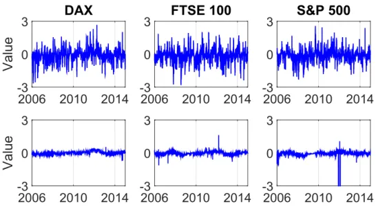
Figure 3: Estimated parameter αe1,0.01 across the three selected stock markets from

2 January 2006 to 31 December 2014, with 20 (upper panel) and 250 (lower panel) observations used in the rolling window exercise at fixed expectile level τ = 0.01. LCARE_Estimation_Rolling_001

given expectile level τ, there are three potential ’true’ parameter constellations, i.e., the parameters that are most likely to be found in practice.

Estimation Quality

The estimation quality of the quasi-maximum likelihood approach is addressed here. De-note the pseudotrue parameter vector asθ∗_τ at expectile levelτ, the quality of estimating

θ_τ∗ by quasi-maximum likelihood estimator (QMLE)θe_I,τ given in (6) is measured in terms

of the Kullback-Leibler divergence

Eθ∗ τ `I Y;θe<sub>I,τ</sub> −`I(Y;θ∗τ) r ≤ Rr(θτ∗) (7)

with Rr(θτ∗) denoting the risk bound, see, e.g., Mercurio and Spokoiny (2004) and

Spokoiny (2009). In practice the modest risk power r = 0.5 leads to relatively shorter intervals of homogeneity as compared with the conservative risk case withr = 1. Accord-ing to the pseudo true parameter vector, we simulate thousand time series of the CARE specification and take the largest average value of the (r-th power) difference between the respective log-likelihood values, see equation (7), as the corresponding risk bound. Note

τ = 0.05 τ = 0.01

Low Mid High Low Mid High

e α0,τ -0.01514 -0.00998 0.00000 -0.02892 -0.02323 0.00000 e α1,τ -0.01034 0.05234 0.12149 -0.00298 0.10132 0.12637 e α2,τ -0.31360 -0.85700 0.00421 -0.14472 -2.43912 0.00008 e α3,τ -0.06366 0.56274 0.17589 -0.00037 2.63032 0.03325 e σ2 ετ 0.00001 0.00005 0.00007 0.00001 0.00040 0.00004

Table 2: Descriptive statistics of estimated CARE parameters. All estimated CARE parameters based on the window covering one year, i.e., 250 observations, for the three stock market indices from 2 January 2006 to 31 December 2014 (2348 trading days) are pooled together for the two expectile levels τ = 0.05 and τ = 0.01, respectively. We label the first quartile as ’low’, the mean as ’mid’ and the third quartile as ’high’. LCARE_Parameter_Dynamics_Quartiles

that the considered interval candidates in this simulation covered {20,25,31,39,49,61,76,95,119,149,186,250}

observations - see the selection details in the following sub-section.

The simulated risk boundRr(θτ∗) according to equation (7) across different setups is given

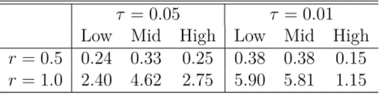
in Table 3. We consider the modest (r= 0.50) and the conservative (r= 1.00) risk case for two expectile levels, τ = 0.05 and τ = 0.01. The risk bounds are obtained by Monte Carlo simulation for each selected parameter vector corresponding to Table 2 where we label the first quartile of estimated parameters as ’low’, the mean as ’mid’ and the third quartile as ’high’. It turns out that the risk bounds in the conservative risk case (r= 1) are relatively larger than the bounds obtained in the modest risk case with r= 0.5.

τ = 0.05 τ = 0.01 Low Mid High Low Mid High

r= 0.5 0.24 0.33 0.25 0.38 0.38 0.15

r= 1.0 2.40 4.62 2.75 5.90 5.81 1.15

Table 3: Risk bound Rr(θτ∗) given two expectile levels, τ = 0.05 and τ = 0.01. We

consider the modest (r= 0.50) and the conservative (r= 1.00) risk case. The risk bounds are obtained by Monte Carlo simulation for each selected parameter vector from Table 2 where we label the first quartile of estimated parameters as ’low’, the mean as ’mid’ and the third quartile as ’high’. LCARE_Risk_Bound_Results

as follows: (a) with different estimation sample windows, a tradeoff between the modelling bias and parameter variability exists, (b) the estimated parameter characteristics as well as the estimation quality results demand a method that successfully accommodates time-varying parameters, (c) data intervals covering 60 to 250 observations may be suitable in providing a good balance between the bias and variability, (d) it is reasonable practice to select three data-driven ’true’ parameter constellations for each expectile level in daily risk management. Motivated by these findings, we now introduce some more details of lCARE.

3.3

Local Parametric Approach

How to account for the time-varying characteristics of CARE parameters in tail risk mod-elling? We utilize the aforementioned local parametric approach (LPA), which has been gradually introduced to modelling time series data in econometrics. The essential idea of lCARE is to find the longest interval over which the CARE model can be approximated by constant parameters.

This interval is labelled as the interval of homogeneity. By a sequential testing procedure, we adaptively select the interval of homogeneity among interval candidates. After the corresponding critical values of the sequential test have been simulated by employing a Monte Carlo method, the adaptive parameter estimate at every time point (i.e., trading day) is selected, based on the test outcome. It is worth noting that at each observation, the associated critical values curve is selected based on a data-driven approach.

Interval Selection

There are many possible candidates for these intervals of homogeneity. To alleviate the computational burden, we choose (K + 1) nested intervals of length nk = |Ik|,

k = 0, . . . , K, i.e., I0 ⊂ I1 ⊂ · · · ⊂ IK. Interval lengths are assumed to be

geometri-cally increasing with nk =

h

n0ck

i

. Based on the empirical results reported above, it is reasonable to select (K+ 1) = 12 intervals, starting with 20 observations (one trading month) and for convenience to end with 250 observations (one trading year), i.e., we consider the set

{20,25,31,39,49,61,76,95,119,149,186,250}.

where within the initial intervalI0 the local CARE model with a constant parameter fits

reasonably well. This shortest interval is therefore assumed to be homogeneous.

Local Change Point Detection Test

Based on the selected nested intervals, we utilize a sequential testing procedure to adap-tively find the homogeneous interval at a fixed data point t0. The initial interval I0 is

assumed to be homogeneous. Consider now Jk=Ik\Ik−1, and sequentially conduct the

test, i.e., over interval index steps k = 1, . . . , K. The hypotheses of the test at step k

read as

H0 : parameter homogeneity of Ik vs H1 :∃ change point withinJk =Ik\Ik−1.

The test statistics is

Tk,τ = sup s∈Jk n `Ak,s Y,θe<sub>A</sub> k,s,τ +`Bk,s Y,θe_B k,s,τ −`Ik+1 Y,θe_I k+1,τ o (8)

where Ak,s = [t0−nk+1, s] and Bk,s = (s, t0] utilize only part of the observation within

the intervalIk+1. Since the change point position is unknown, we test every points ∈Jk.

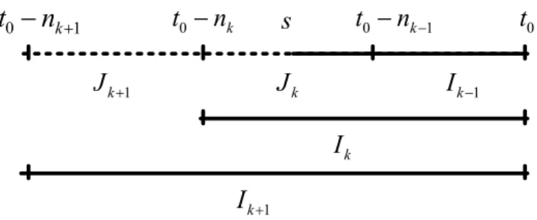
The algorithm at stepk is visualized in Figure 4. Assuming that the null of homogeneity of interval Ik−1 has not been rejected, the testing procedure at step k tests for the

ho-mogenity ofIk. Since the position of a change point withinJk =Ik\Ik−1 is unknown, the

test statistic is calculated based on all pointss∈Jk, i.e. s ∈(t0−nk−1, t0 −nk], utilizing

data from Ik+1. Compute the sum of the log-likelihood values over the sample interval

Ak,s = [t0−nk+1, s] (dotted area) and Bk,s = (s, t0] (solid area) and subtract the

log-likelihood value overIk+1. The likelihood ratio test statistics Tk,τ at each predetermined

expectile level τ is then determined by (8).

The test statistics (8) at every stepkis compared to the corresponding (simulated) critical value zk,τ, for a given expectile and significance level at fix point t0. Then the adaptive

estimate is obained by θb_τ = θe_I

ˆ

k,τ, with bk = max_k≤K {k :T`,τ ≤z`,τ, `≤k}. Here the index and the length of the interval of homogeneity are denoted by kb and n

bk

, respectively. If the null is already rejected at the intervalI1,kb = 0 and similarly, if the null has not been

0 k t n t n0 k1 t₀ 0 k 1

t n



Figure 4: Sequential testing for parameter homogeneity in interval Ik with length nk

ending at fixed time point t0

Critical Values

The critical value sequence zk,τ, k = 1, . . . , K essentially controls the threshold values

of the likelihood ratio test statistic (8). The true distribution of the test statistics is unknown and thus we resort to simulate the critical values. Critical values are calculated through the propagation condition at each step k = 1, . . . , K

Eθ∗ τ `Ik Y;θe<sub>I</sub> k,τ −`Ik Y;θb_τ r ≤ρkRr(θτ∗) (9) with ρk = ρk

K. Here ρ is a false alarm level.

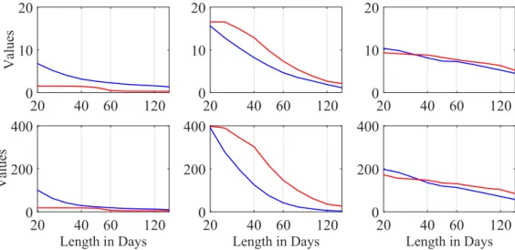
The resulting critical value curves satisfying equation (9) for the selected six ’true’ param-eter constellations from Table 2 and associated risk bounds from Table 3 are displayed in Figure 5. The upper (lower) panel represents critical values in the modest (conservative) risk case. The blue and red lines consider the expectile levels τ = 0.05 and τ = 0.01, respectively. Critical values evolve in a decreasing route, with a similar magnitude across all cases except for the middle ’true’ parameter constellations in the first few steps. It is therefore reasonable to choose the critical value set in a data-driven fashion: at a fixed time point, the yearly estimateαb1,τ serves as a benchmark to select the appropriate curve.

If its value is, for example, higher than the reported upper quartile case in Table 2, then the corresponding critical value curve is selected.

20 40 60 120 Values 0 10 20 20 40 60 120 0 10 20 20 40 60 120 0 10 20 Length in Days 20 40 60 120 Values 0 200 400 Length in Days 20 40 60 120 0 200 400 Length in Days 20 40 60 120 0 200 400

Figure 5: Simulated critical values across different parameter constellations given in Table 2 for the modest (upper panel, r = 0.5) and conservative (lower panel,

r = 1) risk cases. We consider two expectile levels, τ = 0.05 (blue) and τ = 0.01 (red). LCARE_Critical_Values LCARE_Critical_Values_Th1_001 LCARE_Critical_Values_Th1_005 LCARE_Critical_Values_Th2_001 LCARE_Critical_Values_Th2_005 LCARE_Critical_Values_Th3_001 LCARE_Critical_Values_Th3_005

4

Empirical Results

lCARE accommodates and reacts to structural changes. From the fixed rolling window exercise in subsection 3.2 one observes time-varying parameter characteristics while facing the trade-off between parameter variability and the modelling bias. How to account for the effects of potential market changes on the tail risk based on the intervals of homogenity? In this section, we utilize the lCARE model to estimate the tail risk exposure across three stock markets. Using the time series of the adaptively selected interval length, we improve a portfolio insurance strategy employing our tail risk estimate and furthermore enhance its performance in the following application part.

4.1

Intervals of Homogeneity

The interval of homogeneity in tail expectile dynamics is obtained here by the lCARE framework for the time series of DAX, FTSE 100 and S&P 500 returns. Using the sequential local change point detection test, the optimal interval length is considered at two expectile levels, τ = 0.05 and τ = 0.01. We set the significance level ρ = 0.25. Interestingly, the homogeneity intervals are relatively longer at the end of 2009 and at the beginning of 2010 especially atτ = 0.05, the period following the financial crisis across all three stock markets, see, e.g., Figures 6 and 7. Figure 6 presents the estimated length of the interval of homogeneity in trading days across the selected three stock market indices from 2 January 2006 to 31 December 2014 at the expectile level τ = 0.05, while Figure 7 denotes the results givenτ = 0.01. The upper panel depicts the modest risk case r= 0.5, whereas the lower panel denotes the conservative risk case r = 1.

Recall that the lCARE model aims to select the longest interval over which the null hypothesis of time homogeneity of CARE parameters is not rejected. In the financial crisis initial period, the homogeneity intervals became shorter, due to the increasing market volatility and obvious market turmoil. During the post-crisis period, characterised by the high volatile regime, the homogeneity intervals became relatively longer.

In a similar way, the intervals of homogeneity are relatively shorter in the modest risk case r= 0.5, as compared to the conservative risk case r= 1. The average daily selected

2006 2010 2014 60 120 180 DAX Length 2006 2010 2014 60 120 180 FTSE 100 2006 2010 2014 60 120 180 S&P 500 2006 2010 2014 60 120 180 DAX Length 2006 2010 2014 60 120 180 FTSE 100 2006 2010 2014 60 120 180 S&P 500

Figure 6: Estimated length of the interval of homogeneity in trading days across the selected three stock markets from 2 January 2006 to 31 December 2014 for the modest (upper panel,r = 0.5) and the conservative (lower panel,r= 1) risk cases. The expectile level equals τ = 0.05. LCARE_Adaptive_Estimation_Length_005

LCARE_Adaptive_Estimation_005 2006 2010 2014 60 120 180 DAX Length 2006 2010 2014 60 120 180 FTSE 100 2006 2010 2014 60 120 180 S&P 500 2006 2010 2014 60 120 180 DAX Length 2006 2010 2014 60 120 180 FTSE 100 2006 2010 2014 60 120 180 S&P 500

Figure 7: Estimated length of the interval of homogeneity in trading days across the selected three stock markets from 2 January 2006 to 31 December 2014 for the modest (upper panel,r = 0.5) and the conservative (lower panel,r= 1) risk cases. The expectile level equals τ = 0.01. LCARE_Adaptive_Estimation_Length_001

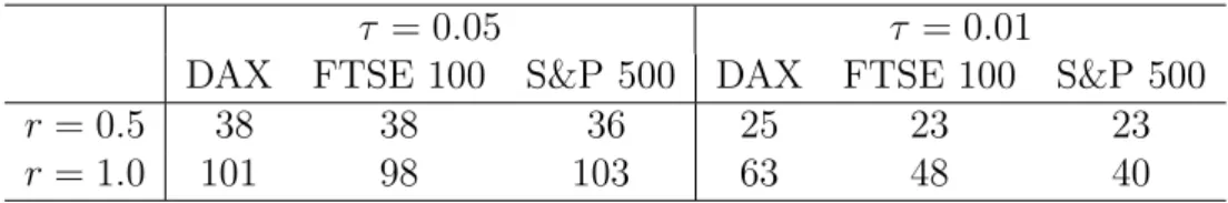
optimal interval length supports this, see, e.g., Table 4. The results are presented for both expectile levels, τ = 0.05 and τ = 0.01, at the modest and the conservative risk cases,

r= 0.50 and r= 1, respectively. At expectile level τ = 0.01, the interval of homogeneity is comparatively shorter than the interval at τ = 0.05, due to more severe tail events. This fact is also implied by the associated parameter variability.

τ = 0.05 τ = 0.01

DAX FTSE 100 S&P 500 DAX FTSE 100 S&P 500

r= 0.5 38 38 36 25 23 23

r= 1.0 101 98 103 63 48 40

Table 4: Mean value of the adaptively selected intervals. Note: the average number of trading days of the adaptive interval length is provided for the DAX, FTSE 100 and S&P 500 market indices at two expectile levels, τ = 0.05 and τ = 0.01, and the modest (r= 0.50) and the conservative (r= 1.00) risk case.

4.2

Dynamic Tail Risk Exposure

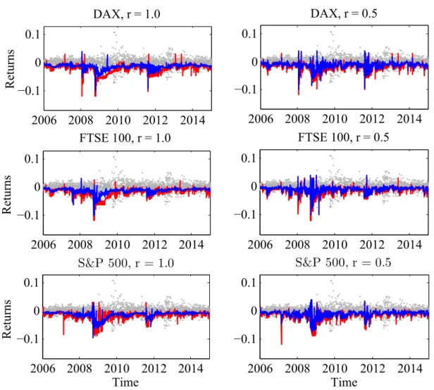
Based on the lCARE model, one can directly estimate dynamic tail risk exposure measures through the adaptively selected intervals. The tail risk at smaller expectile level is lower than risk at higher levels, see, e.g., Figure 8. Here the estimated expectile risk exposure for the three stock market indices from 2 January 2006 to 31 December 2014 is displayed for levels τ = 0.05 and τ = 0.01, respectively. The left panel represents the conservative risk case r = 1 results, whereas the right panel considers the modest risk case r = 0.5. The former leads on average to lower variability, as compared to the modest risk which results in shorter homogeneity intervals.

Estimated expectiles allow us to calculate other tail risk measures, most prominently expected shortfall that represents the expected value of portfolio loss above a certain threshold, e.g., Value at Risk (VaR). The quantile estimation can be improved by em-ploying an expectile-based expected shortfall (ES) framework. In its derivation one notes a one-to-one mapping between quantiles and expectiles with the expectile level τα being

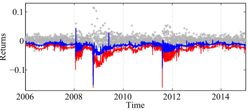
2006 2008 2010 2012 2014 −0.1 0 0.1 Returns DAX, r = 1.0 2006 2008 2010 2012 2014 −0.1 0 0.1 Returns FTSE 100, r = 1.0 2006 2008 2010 2012 2014 −0.1 0 0.1 Time S&P 500, r = 1.0 Returns 2006 2008 2010 2012 2014 −0.1 0 0.1 DAX, r = 0.5 2006 2008 2010 2012 2014 −0.1 0 0.1 FTSE 100, r = 0.5 2006 2008 2010 2012 2014 −0.1 0 0.1 Time S&P 500, r = 0.5

Figure 8: Estimated expectile risk exposure at level τ = 0.05 (blue) and τ = 0.01 (red) for return time series of DAX, FTSE 100, and S&P 500 indices from 2 January 2006 to 31 December 2014. The left panel shows results of the conservative risk case r = 1 and the right panel depicts the results of the modest risk caser = 0.5.

selected such that et,τα =qα, i.e., α-quantile τα = α·qα− Z qα −∞ ydF(y) E[Y]−2 Z qα −∞ ydF(y)−(1−2α)qα (10)

where F (·) denotes the cumulative density function (cdf) of a random variable Y. The corresponding expected shortfall can be expressed as

ESet,τα = 1 +τα(1−2τα) −1 α−1 et,τα (11)

with et,τα denoting the expectile at level τα. In order to apply (11), one needs to fix a certain cdf F (·) in (10). The asymmetric normal distribution is chosen here considering the consistency with the aforementioned model specification.

Consider the tail risk exposure of DAX index series at expectile level τ = 0.05 and conservative risk case r = 1.0. During market distress periods, e.g., the 2008 financial crisis or the 2012 European sovereign debt crisis, the estimated expected shortfall (11) exhibits a high variation, as depicted in Figure 9. Note that the asymmetric normal distribution from subsection 3.1 has been employed in ES calculation. Similarly to current research developments, the estimated expected shortfall using the proposed lCARE model exceeds (by magnitude) the estimated expectileet,τ value.

2006 2008 2010 2012 2014 −0.1 0 0.1 Returns Time

Figure 9: Adaptively estimated expectile (blue) and expected shortfall (red) for DAX index returns from 2 January 2006 to 31 December 2014. We choose r= 1 and τ = 0.05.

4.3

Application: Portfolio Insurance

In practice, dynamic tail risk measures are useful tools in many areas, for example in portfolio insurance - a portfolio protection strategy tailored especially for mutual fund management and portfolio optimization. Particularly, a given proportion of an initial asset portfolio value is preserved at the end of the predetermined time horizon. In this aspect the downside risk is limited under bearish market conditions. Simultaneously, the optimal profit return emerges in bullish market situations and thus fund managers can utilize the time invariant portfolio protection (TIPP) strategy, Estep and Kritzman (1988), Hamidi et al. (2014). It turns out that this represents an extension of the constant proportion portfolio insurance (CPPI) strategy by Black and Jones (1987), Black and Perold (1992).

The CPPI method is applied for a dynamic portfolio allocation along the whole man-agement period. The fund managers firstly predetermine a floor, which is the lowest acceptable portfolio value at the end of the investment horizon, and then invest the ex-posure, the multiple amount of the excess of the portfolio value above the floor by a multiplier, into the risky asset and the remaining part into riskless asset or cash. The TIPP strategy is an extension of the CPPI method, i.e., its floor is time-varying, relat-ing the floor to a proportion of the highest previous portfolio value, which seems more conservative but more actively responds to the prevailing market conditions.

The proportion of the total portfolio invested in risky assets is determined by the so-called asset multiplier. The multiplier is the leverage value of the risky exposure. It is a challenging task to obtain a reasonable multiplier figure. A traditional approach assumes that the multiplier is a constant, i.e., it is insensitive to the current market conditions. Our lCARE model certainly adapts to the risk exposure, say at different states of the economy (bearish or bullish market), and we account for a time-varying nature of the asset multiplier in portfolio allocation. It is expected that during favourable conditions, more assets can be allocated into risky investments and vice versa. The trading idea of the TIPP strategy is explained and thereafter the relationship between the multiplier and the return of the risky asset is derived. The methodologies (constant vs adaptive multiplier selection) are then applied to the DAX index return series and evaluated afterwards.

Time Invariant Portfolio Protection Strategy (TIPP)

Denote the initial asset portfolio value as Vt at time t ∈ (0, T]. An investor aims to

preserve a predetermined protection value F_ts, the so-called floor, at each day

Vt ≥ s×max ( F ·e−rft·(T−t)_{, sup} p≤t Vp ) =F_ts (12)

with an exogenous parameter s ∈(0,1) and the cushion value, Ct =Vt−Fts ≥0. rft is

the risky free rate and we set the initial value F = 100 and the proportion values= 0.9. The allocation decision states thatGt=m·Ctis invested into the risky asset with return

rt (here the DAX portfolio). Herem denotes a non-negative multiplier that controls the

portfolio performance. The remaining amountVt−Gt is invested into a riskless asset.

The portfolio value Vt and consequently the cushion value Ct=Vt−Fts evolve as:

Vt+1 =Vt +Gtrt+1 + (Vt−Gt)rft+1 (13)

Ct+1 =Ct{1 +m·rt+1 + (1−m)rft+1} (14)

Since the cushion value Ct ≥ 0, for all t ≤ T, an upper bound of the multiple m can

be derived from equation (14) when rft is negligibly small and the risky asset return is

negative

m≤−r−_t+1−1, ∀t≤T (15) with r−_t+1 = min(0, rt+1).

Formula (15) reflects a relationship between m and the tail structure of the distribution of rt. When the downside return loss is, for example, 10%, m ≤ 10, and for a downside

of 20%,m ≤5. When the market is bullish, the investor is prone to invest more into the risky asset and vice versa in the bearish situations.

It is worth to note that in the above TIPP strategy, the cushion value is always expected to be near or above zero. This property only holds in the continuous time and assumes that the investor could timely modify their portfolio allocation before a large downside return happens. In practice, fund managers have to account for the risk that the cushion value may be negative since there may happen a unpredictable large downside market crash whereupon the managers fail to reschedule their portfolio allocations in the discontinuous

rebalancing. This risk is known as the gap risk.

How to deal with gap risk and correspondingly calculate the multiplier? There are two common approaches: the first is through the quantile hedging method, see e.g. Föllmer and Leukert (1999), exploiting Value at Risk to imply the multiplier; another method is based on expected shortfall, see e.g. Hamidi et al. (2014), Ameur and Prigent (2014). In the quantile hedging framework, for a given level α, the protection portfolio condition is given by

P (Ct ≥0, ∀t ≤T)≥1−α.

Similar to the derivation of (15), the multiplier can now be expressed as the 1−αquantile of the distribution of rt P mt ≤ −r_t−₊₁−1, ∀t ≤T ≥ 1−α

where the upbound of m with quantile can be obtained by the above equation.

Note that the quantile technique does not take the magnitude of tail risk into account. The expected shortfall is a coherent risk measure and is more suitable to reflect the tail risk. When the investor is prone to more conservative asset allocation, ES is proposed to estimate the multiplier, see Hamidi et al. (2014).

Performance Comparison

Here we employ the lCARE method to estimate the ES in order to deal with the gap risk. The corresponding multiplier selection is expressed by the lCARE-based ES as

mt,τ = ESet,τ −1 (16)

with et,τ denoting the associated expectile value. In the ES calculation, the data process

follows an asymmetric normal distribution. The conditional multiplier is the inverse of the expected shortfall. In practice, a threshold range for mt,τ ∈ {1,2, . . .12} is used. Figure

10 presents the dynamics of the implied multiplier for the DAX index corresponding to ES in Figure 9 based on the lCARE model withr= 1 and τ = 0.05 from 2 January 2006 to 31 December 2014.

2006 2008 2010 2012 2014 4 8 12 Multiplier Time

Figure 10: Time-varying multiplier mt,τ for DAX index returns corresponding to the

expected shortfall in Figure 9 based on lCARE (r = 1 and τ = 0.05) from 2 January 2006 to 31 December 2014 2006 2008 2010 2012 2014 −0.1 0 0.1 Returns 2006 2008 2010 2012 2014 4 8 12 Multiplier Time

Figure 11: Estimated expectile (blue) and expected shortfall (red) by one-year fixed rolling window (upper panel), and the corresponding time-varying multiplier (lower panel) for DAX index returns from 2 January 2006 to 31 December 2014

In order to better understand adaptive estimation window methods, the one-year rolling window estimation strategy is also selected as one of the benchmark models. In Figure 11, the upper panel presents the estimated expectile and ES based on a one-year fixed rolling window estimation while the lower panel shows the corresponding multipliers. The constant multiplier cases (from 1 to 12) are included for benchmark comparisons.

ES can also be implied by the CAViaR framework, one of the popular conditional au-toregressive modeling approaches for Value at Risk. Given that there is a one-to-one mapping between expectiles and quantiles, the expected shortfall can be formulated by the quantile at the corresponding quantile level when the expectile and quantile values are equal, see (10). Here we also list the CAViaR based ES and the corresponding mul-tiplier to implement the insurance strategy as one of the benchmarks. We firstly choose the corresponding quantile level, then illustrate the CAViaR specification from Engle and Manganelli (2004), before presenting the results.

Under the asymmetric normal distribution assumption, given expectile level τ = 0.05, Equation (10) implies the corresponding quantile level α = 0.065. While Engle and Manganelli (2004) state four CAViaR model specifications, the following asymmetric slope pattern is selected, which appears similar to the focused model specification equation (2),

yt=qt,α+εt,α Quantα(εt,α|Ft−1) = 0 (17)

qt,α =β0+β1qt−1,α+β2y+t−1+β3yt−−1 (18)

where qt,α denotes quantile (VaR) at α ∈(0,1), and Quantα(εt,α|Ft−1) is the α-quantile

of εt,α conditional on the information set Ft−1. In addition, we choose α = 0.065 such

that eτα =qα when τα = 0.05 under the AND assumption.

The estimated quantile (expectile) and ES based on a one-year rolling window estimation associated to the abovementioned CAViaR model (18), in which ES is implied from equation (11) with the quantile (expectile) value, is presented in the upper panel in Figure 12, while the lower panel shows the corresponding multipliers.

The initial value and the target value of a hypothetical portfolio at the end of the one year investment horizon are both set to 100 (F = 100 in equation (12)). Associated to

2006 2008 2010 2012 2014 −0.1 0 0.1 Returns 2006 2008 2010 2012 2014 4 8 12 Multiplier Time

Figure 12: Estimated VaR (blue) (α = 0.065) and expected shortfall (red) by CAViaR -based one-year rolling (upper panel), and the corresponding multiplier (lower panel) for DAX index returns from 2 January 2006 to 31 December 2014

the cushioned portfolio strategy, the daily asset allocation decision at time t is to invest the multiple amount of the difference between the portfolio value and the discounted floor up to t into the stock portfolio (DAX), the rest into a riskless asset. Figure 13 presents the performance of the portfolio value based on the cushioned portfolio strategy with unconditional constant multiplier and the conditional time-varying multiplier for the one-year investment horizon. The black line represents the DAX index, the blue line represents the cushioned portfolio with lCARE based conditional dynamic multiplier, the green line represents the portfolio value using a one-year fixed rolling window estimated multiplier, and the brown line presents the value under CAViaR based one-year rolling estimated multiplier. The comparatively best performed portfolio among the constant multipliers considers m= 5, denoted by the red line.

The cushioned portfolio with the dynamic multiplier closely tracks the observed DAX index and, by construction, simultaneously guarantees the target portfolio value floor at the end of the investment horizon at every trading day, see Figure 13. It is worth noting that the lCARE strategy does very well in comparison to the cushioned portfolio with a constant multiplier, the one-year rolling window estimation based on expectile or

2006 2008 2010 2012 2014 100 150 200 Price Index Time

Figure 13: Performance of the portfolio value: (a) DAX index (black), (b) m = 5 (red), (c) one-year rolling approach (green), (d) CAViaR based one-year rolling approach (α= 0.065) (brown), (e) mt,τ - lCARE (blue) from 2 January 2006 to 31 December 2014.

quantile.

Table 5 furthermore presents the return moment performance of the portfolio insurance strategy. We list the statistical results of empirical data, the TIPP strategy with lCARE - based multiplier, one-year fixed rolling window CARE - implied multiplier, one-year rolling window CAViaR implied multiplier, and constant multipliers. The average re-turn of lCARE based strategy, 7.36% is larger than the counterpart based on a fixed rolling window, 5.70%. It is also observed that the CAViaR based strategy performs less favourable. Although, the lCARE strategy is slightly lower than the empirical DAX return of 8.79%, it turns out that it performs favourable relative to other benchmark strategies.

5

Conclusions

The localized conditional autoregressive expectiles (lCARE) model accounts for time-varying parameter characteristics and potential structure changes in tail risk exposure modelling. The parameter dynamics implied by a fixed rolling window exercise of three stock market indices, DAX, FTSE 100 and S&P 500, indicates that there is a trade-off between the modelling bias and parameter variability. A local parametric approach (LPA) assumes that locally one can successfully fit a parametric model. Based on a sequential

Return(%) Volatility(%) VaR 99% Skewness Kurtosis Sharpe Data 8.79 22.54 -4.24 0.24 10.33 0.02 lCARE 7.36 13.60 -2.31 0.52 9.16 0.03 Rolling one-year 5.70 10.18 -1.59 0.17 10.05 0.04 CAViaR rolling 0.01 7.35 -1.43 -0.90 13.04 0.00 Multiplier 1 3.51 2.25 -0.41 0.20 10.05 0.10 Multiplier 2 3.97 4.50 -0.84 0.19 10.00 0.06 Multiplier 3 4.41 6.74 -1.27 0.17 9.90 0.04 Multiplier 4 4.78 9.00 -1.71 0.15 9.88 0.03 Multiplier 5 4.86 11.17 -2.10 0.11 9.91 0.03 Multiplier 6 3.36 5.36 -0.99 -0.33 6.48 0.04 Multiplier 7 2.65 6.04 -1.08 -0.51 6.49 0.03 Multiplier 8 2.13 6.55 -1.17 -0.59 7.90 0.02 Multiplier 9 1.70 6.96 -1.25 -0.74 10.38 0.02 Multiplier 10 1.46 7.33 -1.38 -0.93 12.90 0.01 Multiplier 12 0.82 7.56 -1.47 -1.25 16.65 0.01

Table 5: Descriptive statistics of the portfolio returns based on the TIPP strategy. We employ several models: the lCARE, one-year rolling window, CAViaR rolling window and constant muliplier approach for the DAX index from 2 January 2006 to 31 December 2014. The investment strategy is based on a one-year investment horizon.

testing procedure, one determines the interval of homogeneity over which a parametric model can be approximated by a constant parameter vector.

The lCARE model adaptively estimates the tail risk exposure by relying on the (in-sample) ’optimal’ interval of homogeneity. Setting the expectile levels τ = 0.05 and

τ = 0.01, the dynamic expectile tail risk measures for the selected three stock markets are successfully obtained by lCARE. Furthermore, ES has been introduced, evaluated and employed in the asset allocation example: the portfolio protection strategy is improved by the lCARE modelling framework.

References

Acerbi, C. and Tasche, D. (2002). Expected Shortfall: a natural coherent alternative to Value at Risk, Economic notes31(2): 379–388.

Artzner, P., Delbaen, F., Eber, J. and Heath, D. (1999). Coherent Measures of Risk,

Mathematical Finance9: 203–228.

Black, F. and Jones, R. W. (1987). Simplifying portfolio insurance, The Journal of

Portfolio Management 14(1): 48–51.

Black, F. and Perold, A. F. (1992). Theory of constant proportion portfolio insurance,

Journal of Economic Dynamics and Control 16(3): 403–426.

Cai, Z. and Xu, X. (2008). Nonparametric Quantile Estimation for Dynamic Smooth Coefficient Models, Journal of the American Statistical Association 103(492): 1595– 1608.

Chen, Y., Härdle, W. K. and Pigorsch, U. (2010). Localized Realized Volatility, Journal

of the American Statistical Association105(492): 1376–1393.

Chen, Y. and Niu, L. (2014). Adaptive dynamic Nelson–Siegel term structure model with applications,Journal of Econometrics 180(1): 98–115.

Čížek, P., Härdle, W. K. and Spokoiny, V. (2009). Adaptive pointwise estimation in time-inhomogeneous conditional heteroscedasticity models, Econometrics Journal 12: 248– 271.

De Rossi, G. and Harvey, A. (2009). Quantiles, expectiles and splines, Journal of

Econo-metrics 152(2): 179–185.

Efron, B. (1991). Regression percentiles using asymmetric squared error loss, Statistica

Sinica1(1): 93–125.

Engle, R. F. and Manganelli, S. (2004). CAViaR: Conditional autoregressive value at risk by regression quantiles,Journal of Business & Economic Statistics 22(4): 367–381. Estep, T. and Kritzman, M. (1988). TIPP: Insurance without complexity, The Journal

of Portfolio Management14(4): 38–42.

Föllmer, H. and Leukert, P. (1999). Quantile hedging,Finance and Stochastics3(3): 251– 273.

Gerlach, R. and Chen, C. W. (2014). Bayesian expected shortfall forecasting incor-porating the intraday range, Journal of Financial Econometrics pp. to appear, doi: 10.1093/jjfinec/nbu022.

Gerlach, R. H., Chen, C. W. S. and Lin, L. Y. (2012). Bayesian GARCH Semi-parametric Expected Shortfall Forecasting in Financial Markets, Business Analytics Working

Pa-per No. 01/2012 .

Hamidi, B., Maillet, B. and Prigent, J. L. (2014). A dynamic autoregressive expectile for time-invariant portfolio protection strategies, Journal of Economic Dynamics and

Control 46: 1–29.

Härdle, W. K., Hautsch, N. and Mihoci, A. (2015). Local Apative Multiplicative Error Models for High-Frequency Forecasts,Journal of Applied Econometrics30(4): 529–550. Honda, T. (2004). Quantile Regression in Varying Coefficient Models, Journal of

Statis-tical Planning and Inference121: 113–125.

Inoue, A., Jin, L. and Rossi, B. (2014). Window selection for out-of-sample forecasting with time-varying parameters, CEPR Discussion Paper No. DP10168.

Jones, M. C. (1994). Expectiles and M-quantiles are quantiles, Statistics & Probability

Letters 20(2): 149–153.

Jorion, P. (2000). Value at risk: The new benchmark for managing market risk, McGraw-Hill, 2nd edition, New York.

Kim, M. O. (2007). Quantile Regression With Varying-Coefficients,The Annals of Statis-tics 35(2): 92–108.

Kuan, C. M., Yeh, J. H. and Hsu, Y. C. (2009). Assessing value at risk with CARE, the Conditional Autoregressive Expectile models, Journal of Econometrics 150(2): 261– 270.

Mercurio, D. and Spokoiny, V. (2004). Statistical inference for time-inhomogeneous volatility models, The Annals of Statistics32(2): 577–602.

Pesaran, M. H. and Timmermann, A. (2007). Selection of estimation window in the presence of breaks,Journal of Econometrics 137(1): 134–161.

Spokoiny, V. (1998). Estimation of a function with discontinuities via local polynomial fit with an adaptive window choice, The Annals of Statistics26(4): 1356–1378.

Spokoiny, V. (2009). Multiscale local change point detection with applications to Value-at-Risk, The Annals of Statistics37(3): 1405–1436.

Taylor, J. W. (2008). Estimating Value at Risk and Expected Shortfall Using Expectiles,

Journal of Financial Econometrics6(2): 231–252.

Xie, S., Zhou, Y. and Wan, A. T. (2014). A varying-coefficient expectile model for estimating Value at Risk,Journal of Business & Economic Statistics 32(4): 576–592. Yao, Q. and Tong, H. (1996). Asymmetric least squares regression estimation: a

SFB 649 Discussion Paper Series 2015

For a complete list of Discussion Papers published by the SFB 649, please visit http://sfb649.wiwi.hu-berlin.de.

001 "Pricing Kernel Modeling" by Denis Belomestny, Shujie Ma and Wolfgang Karl Härdle, January 2015.

002 "Estimating the Value of Urban Green Space: A hedonic Pricing Analysis of the Housing Market in Cologne, Germany" by Jens Kolbe and Henry Wüstemann, January 2015.

003 "Identifying Berlin's land value map using Adaptive Weights Smoothing" by Jens Kolbe, Rainer Schulz, Martin Wersing and Axel Werwatz, January 2015.

004 "Efficiency of Wind Power Production and its Determinants" by Simone Pieralli, Matthias Ritter and Martin Odening, January 2015.

005 "Distillation of News Flow into Analysis of Stock Reactions" by Junni L. Zhang, Wolfgang K. Härdle, Cathy Y. Chen and Elisabeth Bommes, Janu-ary 2015.

006 "Cognitive Bubbles" by Ciril Bosch-Rosay, Thomas Meissnerz and Antoni Bosch-Domènech, February 2015.

007 "Stochastic Population Analysis: A Functional Data Approach" by Lei Fang and Wolfgang K. Härdle, February 2015.

008 "Nonparametric change-point analysis of volatility" by Markus Bibinger, Moritz Jirak and Mathias Vetter, February 2015.

009 "From Galloping Inflation to Price Stability in Steps: Israel 1985–2013" by Rafi Melnick and till Strohsal, February 2015.

010 "Estimation of NAIRU with Inflation Expectation Data" by Wei Cui, Wolf-gang K. Härdle and Weining Wang, February 2015.

011 "Competitors In Merger Control: Shall They Be Merely Heard Or Also Listened To?" by Thomas Giebe and Miyu Lee, February 2015.

012 "The Impact of Credit Default Swap Trading on Loan Syndication" by Daniel Streitz, March 2015.

013 "Pitfalls and Perils of Financial Innovation: The Use of CDS by Corporate Bond Funds" by Tim Adam and Andre Guettler, March 2015.

014 "Generalized Exogenous Processes in DSGE: A Bayesian Approach" by Alexander Meyer-Gohde and Daniel Neuhoff, March 2015.

015 "Structural Vector Autoregressions with Heteroskedasticy" by Helmut Lütkepohl and Aleksei Netšunajev, March 2015.

016 "Testing Missing at Random using Instrumental Variables" by Christoph Breunig, March 2015.

017 "Loss Potential and Disclosures Related to Credit Derivatives – A Cross-Country Comparison of Corporate Bond Funds under U.S. and German Regulation" by Dominika Paula Gałkiewicz, March 2015.

018 "Manager Characteristics and Credit Derivative Use by U.S. Corporate Bond Funds" by Dominika Paula Gałkiewicz, March 2015.

019 "Measuring Connectedness of Euro Area Sovereign Risk" by Rebekka Gätjen Melanie Schienle, April 2015.

020 "Is There an Asymmetric Impact of Housing on Output?" by Tsung-Hsien Michael Lee and Wenjuan Chen, April 2015.

021 "Characterizing the Financial Cycle: Evidence from a Frequency Domain Analysis" by Till Strohsal, Christian R. Proaño and Jürgen Wolters, April 2015.

SFB 649, Spandauer Straße 1, D-10178 Berlin http://sfb649.wiwi.hu-berlin.de

SFB 649 Discussion Paper Series 2015

For a complete list of Discussion Papers published by the SFB 649, please visit http://sfb649.wiwi.hu-berlin.de.

022 "Risk Related Brain Regions Detected with 3D Image FPCA" by Ying Chen, Wolfgang K. Härdle, He Qiang and Piotr Majer, April 2015.

023 "An Adaptive Approach to Forecasting Three Key Macroeconomic Varia-bles for Transitional China" by Linlin Niu, Xiu Xu and Ying Chen, April 2015.

024 "How Do Financial Cycles Interact? Evidence from the US and the UK" by Till Strohsal, Christian R. Proaño, Jürgen Wolters, April 2015.

025 "Employment Polarization and Immigrant Employment Opportunities" by Hanna Wielandt, April 2015.

026 "Forecasting volatility of wind power production" by Zhiwei Shen and Matthias Ritter, May 2015.

027 "The Information Content of Monetary Statistics for the Great Recession: Evidence from Germany" by Wenjuan Chen and Dieter Nautz, May 2015. 028 "The Time-Varying Degree of Inflation Expectations Anchoring" by Till

Strohsal, Rafi Melnick and Dieter Nautz, May 2015.

029 "Change point and trend analyses of annual expectile curves of tropical storms" by P.Burdejova, W.K.Härdle, P.Kokoszka and Q.Xiong, May 2015.

030 "Testing for Identification in SVAR-GARCH Models" by Helmut Luetkepohl and George Milunovich, June 2015.

031 "Simultaneous likelihood-based bootstrap confidence sets for a large number of models" by Mayya Zhilova, June 2015.

032 "Government Bond Liquidity and Sovereign-Bank Interlinkages" by Sören Radde, Cristina Checherita-Westphal and Wei Cui, July 2015. 033 "Not Working at Work: Loafing, Unemployment and Labor Productivity"

by Michael C. Burda, Katie Genadek and Daniel S. Hamermesh, July 2015.

034 "Factorisable Sparse Tail Event Curves" by Shih-Kang Chao, Wolfgang K. Härdle and Ming Yuan, July 2015.

035 "Price discovery in the markets for credit risk: A Markov switching ap-proach" by Thomas Dimpfl and Franziska J. Peter, July 2015.

036 "Crowdfunding, demand uncertainty, and moral hazard - a mechanism design approach" by Roland Strausz, July 2015.

037 ""Buy-It-Now" or "Sell-It-Now" auctions : Effects of changing bargaining power in sequential trading mechanism" by Tim Grebe, Radosveta Ivanova-Stenzel and Sabine Kröger, August 2015.

038 "Conditional Systemic Risk with Penalized Copula" by Ostap Okhrin, Al-exander Ristig, Jeffrey Sheen and Stefan Trück, August 2015.

039 "Dynamics of Real Per Capita GDP" by Daniel Neuhoff, August 2015. 040 "The Role of Shadow Banking in the Monetary Transmission Mechanism

and the Business Cycle" by Falk Mazelis, August 2015.

041 "Forecasting the oil price using house prices" by Rainer Schulz and Mar-tin Wersing, August 2015.

042 "Copula-Based Factor Model for Credit Risk Analysis" by Meng-Jou Lu, Cathy Yi-Hsuan Chen and Karl Wolfgang Härdle, August 2015.

043 "On the Long-run Neutrality of Demand Shocks" by Wenjuan Chen and Aleksei Netsunajev, August 2015.

SFB 649, Spandauer Straße 1, D-10178 Berlin http://sfb649.wiwi.hu-berlin.de

This research was supported by the Deutsche

SFB 649 Discussion Paper Series 2015

For a complete list of Discussion Papers published by the SFB 649, please visit http://sfb649.wiwi.hu-berlin.de.

044 "The (De-)Anchoring of Inflation Expectations: New Evidence from the Euro Area" by Laura Pagenhardt, Dieter Nautz and Till Strohsal, Septem-ber 2015.

045 "Tail Event Driven ASset allocation: evidence from equity and mutual funds’ markets" by Wolfgang Karl Härdle, David Lee Kuo Chuen, Sergey Nasekin, Xinwen Ni and Alla Petukhina, September 2015.

046 "Site assessment, turbine selection, and local feed-in tariffs through the wind energy index" by Matthias Ritter and Lars Deckert, September 2015.

047 "TERES - Tail Event Risk Expectile based Shortfall" by Philipp Gschöpf, Wolfgang Karl Härdle and Andrija Mihoci, September 2015.

048 "CRIX or evaluating Blockchain based currencies" by Wolfgang Karl Härdle and Simon Trimborn, October 2015.

049 "Inflation Co-movement across Countries in Multi-maturity Term Struc-ture: An Arbitrage-Free Approach" by Shi Chen, Wolfgang Karl Härdle, Weining Wang, November 2015.

050 "Nonparametric Estimation in case of Endogenous Selection" by Chris-toph Breunig, Enno Mammen and Anna Simoni, November 2015.

051 "Frictions or deadlocks? Job polarization with search and matching fric-tions" by Julien Albertini, Jean Olivier Hairault, François Langotz and Thepthida Sopraseuthx, November 2015.

052 "lCARE - localizing Conditional AutoRegressive Expectiles" by Xiu Xu, Andrija Mihoci, Wolfgang Karl Härdle, December 2015.

SFB 649, Spandauer Straße 1, D-10178 Berlin http://sfb649.wiwi.hu-berlin.de