Parallel Interior Point Solver for Structured Quadratic Programs: Application to Financial Planning Problems

for Structured Quadratic Programs:

Application to Financial Planning Problems

Jacek Gondzio Andreas Grothey April 15th, 2003

MS-03-001

For other papers in this series see http://www.maths.ed.ac.uk/preprints

Application to Financial Planning Problems

∗

Jacek Gondzio

†

Andreas Grothey

‡

School of Mathematics

The University of Edinburgh

Mayfield Road, Edinburgh EH9 3JZ

United Kingdom.

April 15th, 2003

∗_{Supported by the Engineering and Physical Sciences Research Council of UK, EPSRC grant GR/R99683/01.} †_{Email: [email protected], URL:http://maths.ed.ac.uk/~gondzio/}

‡_{Email: [email protected], URL:http://maths.ed.ac.uk/~agr/}

Abstract

Issues of implementation of a library for parallel interior-point methods for quadratic pro-gramming are addressed. The solver can easily exploitanyspecial structure of the underlying optimization problem. In particular, it allows a nested embedding of structures and by this means very complicated real-life optimization problems can be modeled. The efficiency of the solver is illustrated on several problems arising in the financial planning, namely in the asset and liability management. The problems are modeled as multistage decision processes and by nature lead to specially structured tree-sparse problems. By taking the variance of the random variables into account the problems become nonseparable quadratic programs. A reformulation of the problem is proposed which reduces density of matrices involved and by these means significantly simplifies its solution by an interior point method. The object-oriented parallel solver achieves high efficiency by careful exploitation of the block sparsity of these problems. As a result a problem with 10 million decision variables is solved in less than 2 hours on a serial computer. The approach is by nature scalable and the parallel implementation achieves perfect speed-ups.

1

Introduction

We are concerned in this paper with a parallel structure exploiting interior-point solver to tackle the convex quadratic programs (QPs). An advantage of interior point methods (IPMs) is a consistent small number of iterations needed to reach the optimal solution of the problem. Indeed, modern IPMs rarely need more than 20-30 iterations to solve a QP, and this number does not increase significantly even for problems with millions of decision variables. However, a single iteration of interior-point method may be costly because it involves solving large and potentially difficult systems of linear equations. Indeed, the efficiency of interior point methods for quadratic programming critically depends on the implementation of the linear algebra operations.

We deal with the primal-dual interior-point method in this paper. It is widely accepted [2, 27] that the primal-dual algorithm is usually faster and more reliable than the pure primal or pure dual method. The primal-dual method is applied to the primal-dual formulation of the quadratic program

Primal Dual

min cTx+1₂xTQx max bTy−1₂xTQx

s.t. Ax=b, s.t. ATy+s−Qx=c,

x≥0; y free, x, s≥0,

whereA∈ Rm×n_{, Q∈ R}n×n_{,x, s, c∈ R}n _{andy, b∈ R}m_{. The main computational effort of this} algorithm consists in the computation of the primal-dual Newton direction. Applying standard transformations [27] leads to the following linear system to be solved at each iteration

−Q−Θ−1 AT A 0 ∆x ∆y = r h , (1)

where Θ = XS−1 _{and X and S are diagonal matrices in R}n×n _{with elements of vectors x and}

sspread across the diagonal, respectively.

In this paper we are interested in the case where A and Q are large, block-sparse matrices, indeed we assume them to be of a nested block-sparse structure. We note that an augmented system matrix such as in (1) whose componentsA,Qare nested block-structured matrices can be naturally reordered by symmetric row and column permutations (provided the structures of A and Q are compatible), such that the resulting matrix is again a nested block-structured matrix whose elementary blocks are of augmented system type. Thus the structures of A and

Qimply in a natural way a structure of the augmented system matrix.

The approach presented in this paper incorporates in a solver a set of routines that can support

any structure. These are used in an object-oriented implementation which is an extension of [15, 13]. We assume that the structured matrices A and Q are built of a nested set of blocks. The hierarchy of blocks can be naturally represented as a tree: its root is the whole matrix, intermediate nodes are block-structured submatrices and the leaves are the elementary blocks. Our approach takes advantage of inclusion polymorphism: we define a general abstract Matrix

interface for matrix operations of which all other classes (one for each type of block-structured matrix supported) are implementations. This abstractMatrixinterface contains a set of virtual functions (methods in the object-oriented terminology) that:

• provide all the necessary linear algebraic operations for an IPM, and • allow self-referencing.

Among derived classes we define elementary ones for simple sparse and dense matrices as well as classes for block-structured matrices such as block-diagonal, block-sparse, block-dense and block bordered diagonal (which includes as special cases primal angular and dual block-angular matrices). Definitions of block-structured matrices use only references to the abstract

Matrixinterface . This self-referential property of our block-structured matrix classes allows us to represent a variety of nested structures. Block-matrix operations are natural candidates for parallelization. We have therefore implemented all higher-level matrix classes in parallel. The parallelization is coarse-grained and so is well suited to large scale applications.

Further our implementation is effectively providing a linear algebra library for IPMs for QP. It is therefore possible to completely separate the linear algebra part and the IPM logic part of the algorithm.

To illustrate the potential of the new solver, we apply it to solve multistage stochastic quadratic programs arising in financial planning problems, namely in asset liability management. Such problems have drawn a lot of attention in the literature and have often been modeled as multi-stage stochastic linear programs [7, 9, 10, 18, 20, 28, 29]. In this paper we consider an extension in which the risk associated with the later stages is taken into account in the optimization prob-lem. This is achieved by adding the variance term to the original objective of the problem and leads to a QP formulation.

Multistage stochastic linear programs can be solved by the specialized decomposition algorithms [3, 12, 14, 19, 22] or by the specialized interior point implementations [4, 17, 26]. Recently a number of interesting specialized approaches have been proposed for multistage quadratic pro-grams. Steinbach [23] exploits the tree-structure of such problems inherited from the scenario tree of the multistage problem to implicitly reorder the computations in the context of interior point method. Blomvall and Lindberg [5, 6] interpret the problem as an optimal control one and derive the special order in which computations in IPMs should be executed. This approach originates from differential equations and the authors call it the Riccati type method. Parpas and Rustem [21] extend the nested Benders decomposition to handle stochastic quadratic pro-gramming problems and use an IPM-based solver to solve all subproblems.

The origin of our approach is different: we assume that a QP problem is given withany block-structure in it (the block-structure does not have to be the consequence of dynamics and/or uncer-tainty) and we extend OOPS1_{, the object-oriented LP solver [15, 13] to tackle QP problems.}

Multistage stochastic QPs are only one class of problems (among many others) which can be efficiently dealt with the QP extension of OOPS.

The approach presented in this paper is an extension of that implemented in OOPS [15, 13]. The main difference is that in OOPS [15] linear problems were considered so the augmented system of linear equations (1) did not contain matrixQand was always reduced to normal equations

AΘAT∆y=AΘr+h. (2)

1_{The acronym OOPS stands for Object-Oriented Parallel Solver} http://www.maths.ed.ac.uk/~gondzio/parallel/solver.html

This was a viable reduction step because matrix Q was not present in the augmented system and Θ was a diagonal matrix. In the context of quadratic programming such a reduction would lead to almost completely dense normal equationsA(Q+ Θ−1)−1AT and would be likely to incur prohibitively expensive computations (unless Qis a diagonal matrix). Hence in this paper and more generally in the QP extension of OOPS we always deal with the augmented system (1). Another contribution of our paper is the analysis of the influence of the QP problem formulation on the efficiency of the solution process. We propose a nonconvex reformulation of the problem which reduces density of matrices involved and is better suited to the use of IPMs.

The paper is organized as follows. In Section 2 we briefly discuss the linear algebraic opera-tions required to implement the interior-point method for QP. We give examples of the types of structures we wish to exploit and discuss how to exploit them. In Section 3 we introduce the tree representation of the block-structured matrices and discuss certain features of the abstract

Matrixinterface , the crucial object used in our design to support the notion of block. Section 4 reviews the Asset and Liability Management problem, which we use as an example to demon-strate the efficiency of the code. Two different formulations are given, one convex and dense, the other nonconvex but sparse. Section 5 states the actual computational results achieved with our code both in serial and in parallel, while in the final Section 6 we draw our conclusions.

2

Linear Algebra Kernel in the QP Solver

2.1

Linear Algebra in the Interior Point Method for QP

The basis for our implementation is the primal-dual interior point algorithm with multiple centrality correctors [1]. The main computational effort of this algorithm consists in the com-putation of the primal-dual Newton direction. This requires solving the following linear system

−Q−X−1S AT A 0 ∆x ∆y = ξd−X−1ξµ ξp , (3) where ξp = b−Ax, ξd = c−ATy−s+Qx, ξµ = µe−XSe.

The matrix involved in (3) is symmetric but indefinite (even for a convex problems when Qis positive definite). For the sake of accuracy and efficiency, the matrix in the reduced Newton system is regularized with diagonal terms Rp and Rd

H = −Q−X−1S AT A 0 + −Rp 0 0 Rd (4) to obtain a quasidefinite matrix [25]. The use of primal-dual regularization (4) guarantees the existence of a Cholesky-likeLDLT factorization in which the diagonalDcontains both positive and negative elements. It avoids the need of using the 2×2 pivots required otherwise to decompose an indefinite matrix [8, 11].

The matrix in the regularized augmented system (4) is symmetric and quasi-definite (with n

negative pivots, corresponding to theQpart of the matrix andmpositive pivots, corresponding to the A part). In our implementation of interior point method system (3) is regularized and then solved in two steps: (i) factorization of the form LDLT and (ii) backsolve to compute the directions (∆x,∆y). Since the triangular decomposition exists for any symmetric row and column permutation of the quasidefinite matrix [25], the symbolic phase of the factorization (reordering for sparsity and preparing data structures for sparse triangular factor) can be done before the optimization starts.

2.2

Block-Structured Matrices

In this section we give an example of exploitable structures in matricesQand A. We show how by rearranging linear algebra operations a large structured linear system can be reduced to a sequence of small linear systems.

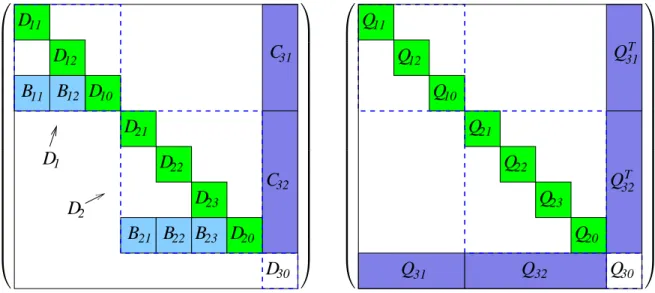
Assume that matrices A and Q are of the structure displayed in Figures 1 and 2, that is a combination of primal-dual block angular, border diagonal and diagonal structures. Then the matrix Φ =

−Q−Θ−1 AT

A 0

can be reordered into the form displayed in Figure 3, i.e. a nested bordered diagonal form (the tilde in ˜C31 for example denotes that this is a part of the

originalC31 matrix). This reordering is generic, i.e. not depending on the particular structure

of Aand Q. In fact it can be seen that the matrix Φ in Figure 3 can be obtained directly from

A/AT and Q in Figures 1/2 by interleaving the matrices. Since Θ is a diagonal matrix and it does not change the sparsity pattern, we do not display it in Figure 3.

It is worth noting that since we use a tree structure to represent our matrices, we need no further memory to store the reordered augmented system matrix Φ. Its leaf node matrices are identical to those already present inAandQ. Hence the reordered augmented system is represented by a new tree, reusing the same leaf node matrices that make upAandQ. Of course, due to this, no physical reordering of memory entries has to be done to obtain the reordered augmented system matrix.

2.3

Symmetric Bordered Block-Diagonal Structure

Suppose a block of the augmented system Φ has the symmetric bordered block-diagonal struc-ture. Φ =        Φ1 BT1 Φ2 BT2 . .. .._. Φn BTn B1 B2 · · · Bn Φ0        , (5)

where Φi ∈ Rni×ni, i = 0, ..., n and Bi ∈ Rn0×ni, i= 1, ..., n. Matrix Φ has then N = Pn

i=0ni

rows and columns. Such blocks will appear as seen in Figure 3 as diagonal blocks or root blocks of the augmented system matrix if its componentA and Qblocks are of block-diagonal and/or block-angular structure.

                        

D

10

D

₃₀

D

20 23

D

22

D

21

D

12

D

11

D

C

B

B

B

B

B

D

₁

D

2 21 23 12 11

C

₃₂ 31 22                         

Figure 1: Example of Block-Structured MatrixA.

                         11

Q

₁₂

Q

10

Q

₂₁

Q

22

Q

₂₃

Q

20

Q

₃₀

Q

Q

Q

Q

Q

T T 31 32 32 31                         

Figure 2: Example of Block-Structured MatrixQ.

                                                         T T

D

11

D

30

D

10

D

12

D

11

D

30

D

30

Q

10

D

12

B

B

T

B

B

B

B

~

Q

31 T T T T T T T T T T T T

B

B

12 11 12 11 T T T

D

D

D

D

D

D

21 21 22 22 23 23

D

D

T 20 20

~

Q

31

Q

~

31

Q

~

32

Q

~

32

Q

~

32

Q

~

32

~

C

₃₁T

C

~

31

C

~

31T

C

~

32

C

~

C

~

C

~

T T 32 32 32

C

~

C

~

C

~

~

Q

~

Q

~

Q

T 32 32 32 32 32 32

~

Q

C

~

~

C

~

C

~

C

~

Q

~

Q

~

Q

31 31 31 32 32 31 31 31

Q

Q

Q

Q

21 22 23 20

Q

Q

11 12

Q

₁₀ 21 22

B

23

B

T T T 23 22 21                                                         

With L=        L1 L2 . .. Ln Ln,1 Ln,2 · · · Ln,n Lc        , D=        D1 D2 . .. Dn Dc        and Φi = LiDiLTi (6a) Ln,i = BiL−i TD− 1 i (6b) C = Φ0− n X i=1 BiΦ−i 1B T i (6c) = LcDcLTc (6d)

matrix Φ can be decomposed as

Φ =LDLT. (7)

Because of this (7) can be seen as a (generalized) Cholesky factorization of Φ. We can use this to compute the solution to the system

Φx=b,

wherex= (x1, . . . , xn, x0)T,b= (b1, . . . , bn, b0)T by the following operations:

zi = L−i 1bi, i= 1, . . . , n (8a) z0 = L−c1(b0− n X i=1 Ln,izi) (8b) yi = D−i 1zi, i= 0, . . . , n (8c) x0 = L−cTy0 (8d) xi = L−_i T(yi−LTn,ix0), i= 1, . . . , n (8e)

It is worth noting that the order in which matrix multiplications are performed in (6) and (8) may have a significant influence on the overall efficiency of the solution of equation Φx=b. The sum to computeCin (6c) is best calculated from terms (L−_i 1BT_i )TD_i−1(L−_i 1B_iT), which in turn is best calculated as sparse outer products of the sparse rows ofL−_i1BT

i . Also the matricesLn,iare best not calculated explicitly. InsteadLn,izi in (8b) is most efficiently calculated asBi(L_i−T(D_i−1zi)) and similarly for LT_n,ix0 in (8e). For these reasons we refer to complex factorizations such as

(6/8) as implicitfactorizations.

Summing up, important savings can be achieved in the storage requirements as well as in the efficiency of computations if the linear algebraic operations exploit the block structure of matrix Φ. Last but not least, exploiting block structure allows an almost straightforward parallelization of many of the computational steps when computing the decomposition of Φ and when solving equations with its factorization.

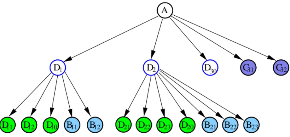
A

D1 D2 D₃₀ C31 C32

D11 D12 D10 B11 B12 D21 D22 D23 D20 B21 B22 B23

Figure 4: Tree Representation of Blocks.

3

Object-Oriented Design

The exploitation of a particular structure could be done with a traditional implementation of IPMs. Then however the code is not easily reusable for other structures. To achieve generality in our design we have followed [15].

There are many structures that can be exploited by an interior-point solver. We restrict our discussion to those in which the matricesAandQare built of blocks and are compatible so that they imply a block structure for the reordered matrix Φ. There are two reasons for that. First, such structures are most often met in practice because they reflect the presence of dynamics, uncertainty, space distribution or other similar factors in the optimization problem. Secondly, block matrix structures can and should be exploited in any optimization algorithm that heavily involves linear algebraic operations, and the interior-point method is such an algorithm.

3.1

Tree Representation of Block-Structured Matrices

With a given block-structured matrix we associate atree that defines the embedding of blocks. Every node in this tree corresponds to a block of the matrix. An arc indicates the embedding of blocks. The root of the tree is the whole matrix, and its leaves correspond to elementary blocks that are not partitioned into smaller entities. Any intermediate node of the tree corresponds to some submatrix that is further partitioned into blocks; the nodes corresponding to these blocks are children of a given node. Figure 4 shows the tree corresponding to the constraints matrixA

in Figure 1.

The tree provides a complete description how the matrix is partitioned. In the example of Fig-ures 1 and 4 the matrix is first partitioned into blocksD1, D2, D30,C31 and C32 corresponding

to dual block-angular structure. Blocks D1 and D2 have primal block-angular structure: they

are partitioned into subblocks D11, D12, D10, B11, B12 and D21, D22, D23, D20, B21, B22, B23,

re-spectively.

With every node of the tree we associate the type of the block-structure. We will say for example that A is a dual block-angular matrix with 2 diagonal blocks, D1 and D2 are primal

block-angular matrices with 2 respectively 3 diagonal blocks, and all the remaining nodes are elementary matrices. Everytype of the block structure corresponds in our layout to a particular implementation of the abstractMatrixinterface .

Observe that the typeof the node determines how the linear algebraic operations for the corre-sponding block of the matrix should be executed. Consider one of the simplest operations such as the matrix-vector product computed with A. The type of node A in the tree implies that the operation will be split into 5 subblocksD1, D2, D30, C31 andC32, corresponding to children

of this node. In cases of nodes D30, C31 and C32 that correspond to elementary blocks, this

operation would invoke a routine appropriate for the given type of the node. For nodesD1 and

D2 the same operation will have to be split further into subblocks — children of nodes D1 and

D2. As seen in Section 2.2 the tree representation of matricesA,Qimplies a tree decomposition

of the augmented matrix Φ.

3.2

Matrix Interface for Augmented System Computations

We use object oriented principles to exploit the structure of matrices A, Q and Φ in the linear algebra operations needed within the interior point method for these matrices. The idea is that linear algebra operations are reduced to operations on nodes of the tree. Every operation for a particular type of matrix is reduced to a combination of operations on the children of this matrix. We have outlined above how this works for matrix-vector products and have given details of the more complexComputeCholeskyandSolveoperations for bordered block-diagonal structure in Section 2.3.

Every type of matrix will correspond to a particular implementation of the abstract Matrix

interface with its particular implementation of the linear algebra methods. In the rest of this section we will discuss the layout of the abstract Matrixinterface .

The abstract Matrix interface provides a general interface to linear algebraic operations sup-ported by any type of matrix. It ensures that every type of matrix supports the same linear algebraic operations and that they can be invoked in a generic way, i.e. without knowing the particular type of the matrix. Every particular type of matrix corresponds to animplementation

of this abstract Matrixinterface , i.e. it provides its specialized implementation of the abstract operations defined in the interface.

To implement an interior point method the following operations with the matrices A, Q and Φ are needed:

• Matrix-vector products M z, MT_{z forA, Q and Φ.} • GivenA, Q and Θ compute Φ.

• Calculate factors Φ =LDLT.

• Solve systemsLz=g,Dz=g and LTz=g.

These operations are an integral part of the abstract Matrix interface used in our solver. It is worth noting that an interior-point algorithm does not need to know how these operations

are executed; it needs to access only theirresults. However this set of routines is not sufficient. This is because the most efficient implementation of some of thesefundamental methods might require further methods to be supported by its child node matrices. E.g. the formation of implicit Cholesky factors by Schur complement (see Section 2.3) requires a method that returns a row or column of the matrix in question.

We therefore introduce a setF_X of methods supported by the abstractMatrixinterface : it has to satisfy a closure condition: any method inF_X can be implemented for any supported matrix structure by only using methods also in F_X on its subblocks.

Below we list the set FX of methods supported by the abstract Matrixinterface : • compute the productM z=g,

• compute the productMT_z=g, • retrieve columnj of M, • retrieve row j ofM, • compute Φ = reorder −Q−Θ−1 AT A 0

for given A,Qand Θ, • compute the inverse representation LDLT = Φ,

• compute the solution of equation Φz=g, • compute the solution of equation Lz=g, • compute the solution of equation Dz=g, • compute the solution of equation LTz=g.

Note that all these operations can be performed by only requiring the results of operations in FX from the subblocks Φi, Bi.

Not all these methods can be sensible used for a particular structure in all circumstances. The “compute Φ” method will only be used if the block is used as part of the constraint matrixA. Similarly the “Compute LDLT” and “Solve” methods will only be applied for blocks used in the augmented system.

3.3

Parallel Implementation

One of the main advantages of an object-oriented linear algebra design is that it lends itself naturally to parallelization. Almost all linear algebra operations for the block-structured matrix types mentioned (e.g. block-bordered diagonal, primal/dual block-angular) can be efficiently computed in parallel, by distributing the blocks among different processors. The object ori-ented design provides a layout that can be adapted for parallel implementation with only minor changes.

Note that we only exploit thiscoarse grain parallelism: In block-structured matrices operations on child-matrices are distributed among processors. No attempt has been made to implement elementary matrices (sparse, dense) in parallel.

4

Asset and Liability Management Problems

There are numerous sources of structured linear programs. Although we have developed a gen-eral structure exploiting IPM solver, we have tested it in the first instance only on Asset/Liability Management (ALM) problems. This section will briefly summarize the structure of these prob-lems. We will follow the problem description of [23, 24] and we refer the reader to [29] and the references therein for a detailed discussion of these problems.

Assume we are interested in finding the optimal way of investing into assets j= 1, . . . , J. The returns on assets are uncertain. An initial amount of cashbis invested att= 0 and the portfolio may be rebalanced at discrete times t= 1, . . . , T. The objective is to maximize the final value of the portfolio at timeT+ 1 and minimize the associated risk measured with the variance of the final wealth. To model the uncertainty in the process we use discrete random eventsωtobserved at times t = 0, . . . , T; each of the ωt has only a finite number of possible outcomes. For each sequence of observed events (ω0, . . . , ωt), we expect one of only finitely many possible outcomes for the next observationωt+1. This branching process creates ascenario treerooted at the initial

event ω0. Let Lt be the level set of nodes representing past observations (ω0, . . . , ωt) at time

t, LT the set of final nodes (leaves) and L = S

tLt the complete node set. In what follows a variable i ∈ L will denote nodes, with i = 0 corresponding to the root and π(i) denoting the predecessor (parent) of node i. Further pi is the total probability of reaching node i, i.e. on each level set the probabilities sum up to one. We draw the reader’s attention to the important issue of scenario tree generation [16].

Let vj be the value of asset j, and ct the transaction cost. It is assumed that the value of the assets will not change throughout time and a unit of assetj can always be bought for (1 +ct)vj or sold for (1−ct)vj. Instead a unit of asset j held in node i (coming from node π(i)) will generate extra returnri,j. Denote byxhi,j the units of assetj held at node iand by xbi,j, xsi,j the transaction volume (buying, selling) of this asset at this node. We assume that we start with zero holding of all assets but with funds b to invest. Further we assume that one of the assets represents cash, i.e. the available funds are always fully invested.

We will now present two slightly different versions of the model resulting from these assumptions. One of them is convex but has a dense Q matrix. The other which is obtained by introducing an extra variable and constraint has a sparseQ matrix at the expense of a nonconvex problem formulation. However the problem is still convex on the null space of the constraints, which is why we use this second formulation due to its sparsity benefits. The non-convexity of the model does not seem to adversely affect the performance of the interior point algorithm.

The objective of the ALM problem is to maximize final wealth while minimizing risk. Final wealthy is simply expressed as the expected value of the final portfolio converted into cash

y=IE((1−ct) J X j=1 vjxhT,j) = (1−ct) X i∈LT pi J X j=1 vjxhi,j,

while risk is expressed as its variance Var((1−ct) J X j=1 vjxhT,j) = X i∈LT pi[(1−ct) X j vjxhi,j−y]2 = X i∈LT pi(1−ct)2[ X j vjxhi,j]2−2y(1−ct) X i∈LT pi J X j=1 vjxhi,j | {z } =y +y2 X i∈LT pi | {z } =1 = X i∈LT pi(1−ct)2[ X j vjxhi,j]2−y2.

The actual objective function of the problem is a linear combination of these two terms as in the Markowitz model [24]. The ALM problem can then be expressed as

max x,y≥0 y−ρ[ X i∈LT pi[(1−ct) X j vjxhi,j]2−y2] s.t. (1−ct) P i∈LTpi P jvjxhi,j = y

(1 +ri,j)xh_π(i),j = xi,jh −xbi,j+xsi,j, ∀i6= 0, j P j(1 +ct)vjxbi,j = P j(1−ct)vjxsi,j, ∀i6= 0 P j(1 +ct)vjxb0,j = b. (9)

If we denotexi= (xsi,1, xbi,1, xhi,1, . . . , xsi,J, xbi,J, xhi,J), and define matrices

A=      1 −1 1 . .. 1 −1 1 −cs₁ cb₁ 0 · · · −cs_J cb_J 0     , Bi =      0 0 1 +ri,1 . .. 0 0 1 +ri,J 0 0 0 · · · 0 0 0      and Qi∈IR3J×3J : (Qi)3j,3k=pi(1−ct)2vjvk, j, k = 1, . . . , J, i∈LT Qi= 0, i6∈LT di∈R1×3J : (di)3j = (1−ct)pivj,

wherecb_j = (1 +ct)vj, csj = (1−ct)vj, we can rewrite problem (9) as max x,y≥0 y−ρ[ X i∈LT xT_i Qixi−y2] s.t. P i∈LTd T i xi = y Bπ(i)xπ(i) = Axi ∀i6= 0 Ax0 = beJ+1. (10)

Now if we assemble the vectorsxi, i∈Landyinto a big vectorx= (y, xσ(0), xσ(1), . . . , xσ(|L|−1))

whereσ is a permutation of the nodes 0, . . . ,|L| −1 in a depth-first order, the problem can be written with a nested block-diagonal Q matrix of the form Q = diag(−1, Qσ(1), . . . , Qσ(|L|−1))

and a constraint matrix Aof the form                      −1 0 di · · · di · · · 0 di · · · di A Bi 0 .. . 0 A Bi A .. . . .. Bi A .. . . .. Bi 0 .. . 0 A Bi A .. . . .. Bi A                      (11)

which is of nested primal/dual block-angular form, resulting in a QP of the form displayed in Figures 1/2/3. However due to the −1 term in the diagonal of Q (while all other Qi — being variance-covariance matrices — are positive semi-definite) this formulation of the problem is not convex.

We can however substitute for the y term in this formulation, using

y2 = [X i∈LT (1−ct)pi J X j=1 vjxhi,j]2 = (1−ct)2 X i∈LT X l∈LT J X j=1 J X k=1 piplvjvkxhi,jxhl,k

resulting in a block-dense Qmatrix with |L| × |L|blocks of the form

Qi,l:    (Qi,l)3j,3k=−(1−ct)2piplvjvk, j, k= 1, . . . , J, i, l∈LT, i6=l (Qi,i)3j,3k= [pi(1−ct)2−(1−ct)2p2i]vjvk, j, k = 1, . . . , J, i∈LT Qi,l= 0, i6∈LT orl6∈LT.

As mentioned before this formulation of the problem is convex (Q now being a variance-covariance matrix) but dense.

Since our algorithm cannot currently exploit the dense Q in this second formulation, we have used the first formulation in our numerical tests. The non-convexity of the problem does not seem to adversely affect the performance of the algorithm.

5

Numerical Results

We shall discuss in this section computational results that illustrate the efficiency of our structure exploiting interior point code for quadratic programming, enabling it to solve QP problems with millions of variables and constraints. Further we demonstrate that the code parallelizes well obtaining almost perfect speed-ups on 2-6 processors.

Problem Stages Blocks Assets Total Nodes constraints variables ALM1 5 10 5 11111 66.667 166.666 ALM2 6 10 5 111111 666.667 1.666.666 ALM3 6 10 10 111111 1.222.222 3.333.331 ALM4 5 24 5 346201 2.077.207 5.193.016 ALM5 4 64 12 266305 3.461.966 9.586.981 UNS1 5 35 5 360152 2.160.919 5.402.296

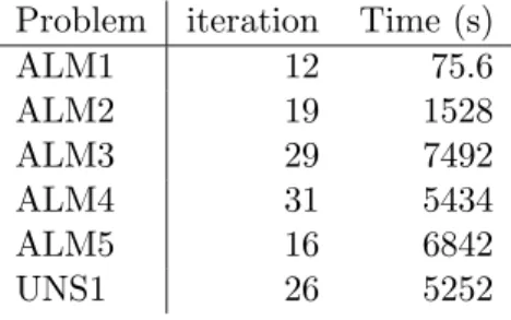
Table 1: Asset and Liability Management Problems: Problem Statistics. Problem iteration Time (s)

ALM1 12 75.6 ALM2 19 1528 ALM3 29 7492 ALM4 31 5434 ALM5 16 6842 UNS1 26 5252

Table 2: Asset and Liability Management Problems: Serial Implementation.

All computations were done on the Sunfire 6800 machine at Edinburgh Parallel Computing Centre (EPCC). This machine features 24 750MHz UltraSparc-III processors and 48GB of shared memory.

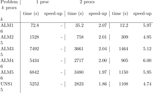
In Table 1 we summarize problem statistics of our test-problems. Further we give solution times and statistics of the serial implementation in Table 2, and finally solution time and speed-up of the parallel implementation is reported in Table 3. While problems ALM1-ALM5 correspond to symmetric scenario trees, problem UNS1 is an example of an unsymmetric scenario tree. In this case the subblocks are distributed among processors by a greedy algorithm (assigning largest subblocks first).

All problems can be solved in a reasonable time and with a reasonable amount of interior point iterations. The speed-up of the parallel implementation is near perfect, due to the exact balance of the blocks treated by each processor and the by far major computational task being distributed amongst the processors. In fact we achieve superlinear speed-up on quite a few problems: we believe this to be the effect of more efficient use of cache when each processor only has to deal with a smaller part of the matrix and the corresponding vectors.

6

Conclusion

We have presented a structure exploiting implementation of an interior point method for quad-ratic programming. Unlike other such implementations which are geared towards one particular type of structure displayed by one particular type of problem, our approach is general enough to exploit any structure and indeed any nested structure. We achieve this flexibility by an object-oriented layout of the linear algebra library used by the method. An additional advantage of

Problem 1 proc 2 procs

kprocs

time (s) speed-up time (s) speed-up time (s) speed-up

k ALM1 72.8 - 35.2 2.07 12.2 5.97 6 ALM2 1528 - 758 2.01 309 4.95 5 ALM3 7492 - 3661 2.04 1464 5.12 5 ALM4 5434 - 2717 2.00 905 6.00 6 ALM5 6842 - 3480 1.97 1150 5.95 6 UNS1 5252 - 2823 1.86 1108 4.74 5

Table 3: Asset and Liability Management Problems: Parallel Implementation.

this layout is that it lends itself naturally to efficient parallelization of the algorithm.

We have given computational results of our algorithm on a selection of randomly generated Asset and Liability Management problems. These problems can be formulated as nonconvex sparse quadratic programs and can be solved very efficiently and with near-perfect speed up in the parallel implementation, enabling us to solve a problem of 10 million variables in about 20 minutes on 6 processors.

References

[1] A. Altman and J. Gondzio,Regularized symmetric indefinite systems in interior point

methods for linear and quadratic optimization, Optimization Methods and Software, 11-12 (1999), pp. 275–302.

[2] E. D. Andersen, J. Gondzio, C. M´esz´aros, and X. Xu,Implementation of interior

point methods for large scale linear programming, in Interior Point Methods in Mathematical Programming, T. Terlaky, ed., Kluwer Academic Publishers, 1996, pp. 189–252.

[3] J. R. Birge,Decomposition and partitioning methods for multistage stochastic linear

pro-grams, Operations Research, 33 (1985), pp. 989–1007.

[4] J. R. Birge and L. Qi,Computing block-angular Karmarkar projections with applications

to stochastic programming, Management Science, 34 (1988), pp. 1472–1479.

[5] J. Blomvall and P. O. Lindberg,A Riccati-based primal interior point solver for

mul-tistage stochastic programming, European Journal of Operational Research, 143 (2002), pp. 452–461.

[6] ,A Riccatibased primal interior point solver for multistage stochastic programming -extensions, Optimization Methods and Software, 17 (2002), pp. 383–407.

[7] S. Bradley and D. Crane, A dynamic model for bond portfolio management, Manage-ment Science, 19 (1972), pp. 139–151.

[8] J. R. Bunch and B. N. Parlett,Direct methods for solving symemtric indefinite systems

of linear equations, SIAM Journal on Numerical Analysis, 8 (1971), pp. 639–655.

[9] D. Cari˜no, T. Kent, D. Myers, C. Stacy, M. Sylvanus, A. Turner, K. Watanabe, and W. Ziemba, The Russel-Yasuda Kasai model: an asset/liability model for Japanese

insurance company using multistage stochastic programming, Interfaces, 24 (1994), pp. 29– 49.

[10] G. Consigli and M. Dempster,Dynamic stochastic programming for asset-liability

man-agement, Annals of Operations Research, 81 (1998), pp. 131–162.

[11] I. S. Duff, A. M. Erisman, and J. K. Reid,Direct methods for sparse matrices, Oxford University Press, New York, 1987.

[12] H. I. Gassmann,MSLiP: A computer code for the multistage stochastic linear programming

problems, Mathematical Programming, 47 (1990), pp. 407–423.

[13] J. Gondzio and A. Grothey,Reoptimization with the primal-dual interior point method, SIAM Journal on Optimization, 13 (2003), pp. 842–864.

[14] J. Gondzio and R. Kouwenberg,High performance computing for asset liability

man-agement, Operations Research, 49 (2001), pp. 879–891.

[15] J. Gondzio and R. Sarkissian, Parallel interior point solver for structured linear

pro-grams, Mathematical Programming, 96 (2003), pp. ??–??

[16] K. Høyland, M. Kaut, and S. W. Wallace,A heuristic for moment-matching scenario

generation, Computational Optimization and Applications, 24 (2003), pp. 169–186.

[17] E. R. Jessup, D. Yang, and S. A. Zenios,Parallel factorization of structured matrices

arising in stochastic programming, SIAM Journal on Optimization, 4 (1994), pp. 833–846. [18] M. Kusy and W. Ziemba, A bank asset and liability model, Operations Research, 34

(1986), pp. 356–376.

[19] J. Linderoth and S. J. Wright,Decomposition algorithms for stochastic programming

on a computational grid, Computational Optimization and Applications, 24 (2003), pp. 207– 250.

[20] J. Mulvey and H. Vladimirou,Stochastic network programming for financial planning

problems, Management Science, 38 (1992), pp. 1643–1664.

[21] P. Parpas and B. Rustem,Decomposition of multistage stochastic quadratic problems in

financial engineering, tech. report, Department of Computing, Imperial College, 2003. Pre-sented at the International Workshop on Comutational Management Science, Economics, Finance and Engineering, Cyprus, 28-30 March, 2003.

[22] A. Ruszczy´nski,A regularized decomposition method for minimizing a sum of polyhedral

functions, Mathematical Programming, 33 (1985), pp. 309–333.

[23] M. Steinbach,Hierarchical sparsity in multistage convex stochastic programs, in Stochastic Optimization: Algorithms and Applications, S. Uryasev and P. M. Pardalos, eds., Kluwer Academic Publishers, 2000, pp. 363–388.

[24] , Markowitz revisited: Mean variance models in financial portfolio analysis, SIAM Review, 43 (2001), pp. 31–85.

[25] R. J. Vanderbei, Symmetric quasidefinite matrices, SIAM Journal on Optimization, 5 (1995), pp. 100–113.

[26] H. Vladimirou and S. A. Zenios,Scalable parallel computations for large-scale stochastic

programming, Annals of Operations Research, 90 (1999), pp. 87–129.

[27] S. J. Wright,Primal-Dual Interior-Point Methods, SIAM, Philadelphia, 1997.

[28] S. Zenios,Asset/liability management under uncertainty for fixed-income securities, An-nals of Operations Research, 59 (1995), pp. 77–97.

[29] W. T. Ziemba and J. M. Mulvey,Worldwide Asset and Liability Modeling, Publications of the Newton Institute, Cambridge University Press, Cambridge, 1998.