A new pattern recognition methodology for classification of load profiles for ships electric consumers

A new pattern recognition

methodology for classification

of load profiles for ships

electric consumers

GJ Tsekouras

1

, IK Hatzilau

1

, JM Prousalidis

1,2

1

_{Hellenic Naval Academy, Department of Electrical Engineering and Computer Science}

2

_{National Technical University of Athens, School of Naval Architecture and Marine}

Engineering, Division of Marine Engineering

In this paper a new pattern recognition methodology is presented for the classification

of the daily chronological load curves of ship electric consumers (equipment) and the

determination of the respective typical load curves of each one of them. It is based on

pattern recognition methods, such as means, adaptive vector quantisation, fuzzy

k-means, self-organising maps and hierarchical clustering, which are theoretically described

and properly adapted. The parameters of each clustering method are properly selected

by an optimisation process, which is separately applied for each one of six adequacy

measures: the error function, the mean index adequacy, the clustering dispersion

indicator, the similarity matrix indicator, the Davies-Bouldin indicator and the ratio of

within cluster sum of squares to between cluster variation. As a study case, this

method-ology is applied to a set of consumers of Hellenic Navy MEKO type frigates.

AUTHORS’ BIOGRAPHIES

Dr GJ Tsekouras (Electrical & Computer Engineer from NTUA/1999, Civil Engineer from NTUA/2004, PhD on Electrical Engineering from NTUA/2006). Adjunct lecturer at the Hellenic Naval Academy, dealing with power system analysis, forecasting and pattern recognition methodologies. Prof Dr-Ing IK Hatzilau (Electrical & Mechanical Engineer from NTUA/1965, Dr-Ing from University of Stuttgart/ 1969). After few years in the industry, he joined the Aca-demic Staff of Dept of Electrical Engineering and Computer Science in Hellenic Naval Academy dealing with marine electrical and control engineering issues. He is representa-tive of Hellenic Navy in NATO AC/141(MCG/6)SG/4 deal-ing with warship-electric systems.

Dr J Prousalidis (Electrical Engineer from NTUA/1991, PhD from NTUA/1997). Assistant Professor at the School of

Naval and Marine Engineering of National Technical Univer-sity of Athens, dealing with electric energy systems and electric propulsion schemes on shipboard installations.

INTRODUCTION

T

he ‘load demand profile’ ie, the chronological energy demand curve is a ‘characteristic para-meter’ of an electric consumer (equipment) of a ship electric network, the value of which vary depending on several factors such as ship type, state, oper-ating modes and mission. In Fig 1 an indicative segment of a daily chronological curve of the refrigeration plant in ship-condition at ‘SHORE’ of HN MEKO type frigate is shown, based on records taken, every 1 min.1

The load demand profile is of primary importance in performing several studies such as load estimation, power sources selection, power cable rating, short circuit analysis,

load shedding, harmonics, modulation etc. The representa-tive load demand profiles of each consumer can be obtained from a classification procedure of its chronological load curves in typical time intervals (also called ‘typical days’). This classification can be conducted by pattern recognition techniques2-6_{, such as:}

- the ‘modified follow the leader’2,4

- the k-means3-4

- the adaptive vector quantisation3 - the fuzzy k-means3-5

- the self-organising map4 - the hierarchical methods3-4.

Regarding adequacy measures commonly used, these can be: - the mean square error3,5

- the mean index adequacy2-3

- the clustering dispersion indicator2-4 - the similarity matrix indicator3

- the Davies-Bouldin indicator3-5

- the modified Dunn index4

- the scatter index4

- the ratio of within cluster sum of squares to between cluster variation.3

Alternatively, the load curves’ classification of consumers can be performed by data mining7_{, wavelet packet}

trans-formation8 _{and Fourier analysis. The last ones are also used}

with simplified clustering models. Conventional tools, like statistical techniques,9 _{need the knowledge of the ‘typical}

days’, which can be defined by experienced ship’s person-nel, eg, chief engineers.

Evidently, one of the major issues of this classification is the definition of the ‘typical day’. In the continental power systems the load curve’s time interval is usually a day for a study time period from a few weeks2to one year.3 In ships’ power systems the corresponding time interval is not defined by any standards, while the total study period can not but be fairly limited (varying from a few days to one month). In this paper the typical time interval is as-sumed to be a day.

In a previous paper,11 _{the authors have thoroughly}

dis-cussed and highlighted the significance of developing such

a methodology in terms of the exploitation of the results yielded to a series of applications and studies of ship systems. In brief, these results, ie, the typical chronological load curves of each consumer, can be used as input infor-mation in:

•

the formalisation of the consumer’s behaviour and the corresponding clustering using the representative load curve of each consumer;

•

the design of the ship’s electric power system estimat-ing the respective total load demand more accurately and, hence selecting the generators properly;

•

the operation of the ship’s power system succeeding more precise short-term load forecasting, increasing the respective reliability and decreasing the respective op-eration cost;

•

the improvement of power factor taking into considera-tion the respective reactive load curves;

•

the load estimation after the application of demand side management programs for each specific consumer, as well as the feasibility studies of the energy efficiency which normalise the total load demand and improve the total load factor;

•

the improvement of the operation of the automatic battle management and load shedding systems, because the automatic supply of the critical consumers in each operating mode is facilitated in case of power system’s fault based on the available generators, the healthy part of the power distribution system and the load demand of each consumer.

The objective of this paper is to present a new methodology for the classification of the daily chronological load curves of ship electric consumers. This method is based on the so-called unsupervised neural networks. More specifically, for each consumer the corresponding set of load curves is organised into well-defined and separate classes, in order to successfully describe the respective demand behaviour with-out any intervention by the user in the classification proce-dure. The proposed methodology compares the results obtained from certain clustering techniques (k-means, adaptive vector quantisation (AVQ), fuzzy k-means, self-organising maps (SOM) and hierarchical methods) using six adequacy measures (mean square error, mean index ade-quacy, clustering dispersion indicator, similarity matrix in-dicator, Davies-Bouldin inin-dicator, ratio of within cluster sum of squares to between cluster variation). The main points of this methodology are:

•

the estimation of the representative typical daily load profiles for each consumer;

•

the modification of the clustering techniques for this kind of classification problem, such as the appropriate weights initialisation for the means and fuzzy k-means;

•

the proper parameters calibration, such as the amount of fuzziness for the fuzzy k-means, in order to fit the classification needs;

•

the comparison of the clustering algorithms perform-ance for each one of the adequacy measures;

•

the selection of the proper adequacy measure.

Fig 1: Indicative chronological energy demand curve of an electric consumer of HN MEKO type frigate

Finally, the results of the application of the developed methodology are thoroughly presented for the case study of six electric consumers of Hellenic Navy MEKO type fri-gates, the chronological load curves of which have been measured within the framework of a research project.1

PROPOSED PATTERN RECOGNITION

METHODOLOGY FOR LOAD CURVES

CLASSIFICATION OF SHIPS ELECTRIC

CONSUMERS

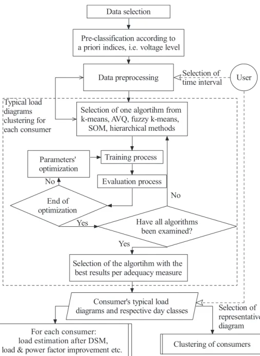
The classification of daily chronological load curves of each ship electric consumer is achieved by applying the pattern recognition methodology shown in Fig 2. The main steps are:

1. Data and features selection: Using electronic meters or ship energy management system for main consumers, the active and reactive power values are recorded (in

kWh and kVArh) for each period in steps of 1min, 15min, etc. The chronological load curves for each individual consumer are determined for each study period (week, month).

2. Consumers’ clustering using a priori indices: Consu-mers can be characterised by their voltage level (high, medium, low), installed power, power factor, load fac-tor, criticality according to ship’s operating mode etc. These indices are not necessarily related to the load curves. They can be used however for the pre-classifi-cation of consumers. It is noted that the load curves of each consumer are normalised using the respective minimum and maximum loads of the period under study.

3. Data preprocessing:The load curves of each consumer are examined for normality, in order to modify or delete the values that are obviously wrong (noise sup-pression). If necessary, a preliminary execution of a pattern recognition algorithm is carried out, in order to trace erroneous measurements or networks faults,

Fig 2: Flow diagram of pattern recognition methodology for the classification of daily chronological load curves of ships electric consumer

which, if uncorrected, will reduce the number of the useful typical time intervals for a constant number of clusters.

4. Typical load curves clustering for each consumer: For each consumer, a number of clustering algorithms (k-means, adaptive vector quantisation, fuzzy k-(k-means, self-organising maps and hierarchical methods) is ap-plied. Each algorithm is trained for the set of load diagrams and evaluated according to six adequacy measures. The parameters of the algorithms are opti-mised, if necessary. The developed methodology uses the clustering methods providing the most satisfactory results. This process is repeated for the total set of consumers under study. Special consumers, such as seasonal or emergency ones (eg, machine tools, fire-pumps, etc) are identified. These results can be com-bined with the ships’ operating mode. At this stage, the size of time interval (1, 2, 3, 4, 6 hours, half or one day) could be investigated, too.

The typical load curves of consumers used are selected by choosing the type of typical time interval (such as the most populated one, the time interval with the peak demand load, etc).

MATHEMATICAL MODELLING OF

CLUSTERING METHODS AND

CLUSTERING VALIDITY ASSESSMENT

General

In the study case of the chronological typical load curves of ship electric consumers, a number ofNanalytical daily load curves is given. The main target is to determine the respec-tive sets of days and load patterns. Generally,N is defined as the population of the input (or training) vectors, which are going to be clustered. ~xx‘¼(x‘1,x‘2,. . .x‘i,. . .x‘d)T

symbolises the‘-th input vector anddits dimension, which equals to 1440 (the load measurements are taken every minute). The corresponding set is given by X ¼ f~xx‘:‘¼1,. . .,Ng. It is worth mentioning that x‘i are

normalised using the higher and lower values of all ele-ments of the original input patterns set, in order to obtain better results from the application of clustering methods.

Each classification process makes a partition of the ini-tial N input vectors to M clusters. The j-th cluster has a representative, which is the respective load profile and is represented by the vector ~wwj¼(wj1,wj2,. . .,wji,. . .,

wjd)T of d dimension. Vector ~wwj expresses the cluster

centre. The corresponding set is the classes set, which is defined by W ¼ f~wwk, k¼1,. . . Mg. The subset of input

vectors~xx‘, which belongs to the j-th cluster, isj and the

respective population of load diagrams is Nj. For the study

and evaluation of classification algorithms the following distance forms are defined:

1. the Euclidean distance between ‘1, ‘2 input vectors of

the setX: dð~xx‘1,~xx‘2Þ ¼ ffiffiffiffiffiffiffiffiffiffiffiffiffiffiffiffiffiffiffiffiffiffiffiffiffiffiffiffiffiffiffiffiffiffiffi 1 d Xd i¼1 x‘1ix‘2i ð Þ2 v u u t (1)

2. the distance between the representative vector ~wwj of

j-th cluster and the subset j, calculated as the

geo-metric mean of the Euclidean distances between~wwjand

each member ofj: d ~wwj,j ¼ ffiffiffiffiffiffiffiffiffiffiffiffiffiffiffiffiffiffiffiffiffiffiffiffiffiffiffiffiffiffiffiffiffiffiffiffiffi 1 Nj X ~xx‘2j d2 ~wwj,~xx‘ s (2)

3. the infra-set mean distance of a set, defined as the geometric mean of the inter-distances between the members of the set, ie, for the subsetj:

^ d dðjÞ ¼ ffiffiffiffiffiffiffiffiffiffiffiffiffiffiffiffiffiffiffiffiffiffiffiffiffiffiffiffiffiffiffiffiffiffiffiffiffiffiffiffi 1 2Nj X ~xx‘2j d2~xx‘,j s (3)

The basic characteristics of the five clustering methods being used are the following.

k-means model

Thek-means method is the simplest hard clustering method, which gives satisfactory results for compact clusters.11 The

k-means clustering method groups the set of the N input vectors to M clusters using an iterative procedure. The re-spective steps of the algorithm are the following:

1. Initialisation of the weights of the M clusters is deter-mined. In the classic model a random choice among the input vectors is used4_{. In the developed algorithm}

thewjiof thej-th centre is initialised as:

w(0)_ji ¼aþb(j1)=(M1) (4) whereaandbare properly calibrated parameters. 2. During training iterationt(called ‘epoch’t,hereinafter)

for each training vector ~xx‘ its Euclidean distances

d(~xx‘,~wwj) are calculated for all centres. The ‘-th input

vector is put in the set (t)_j , for which the distance between ~xx‘ and the respective centre is minimum,

which means:

dð~xx‘,~wwkÞ ¼min

8j d ~xx‘,~wwj

(5) 3. When the entire training set is formed, the new weights

of each centre are calculated as:

~ww(t_jþ1)¼ 1

N(t)_j

X

~xx‘2(jt)

~xx‘ (6)

where N(_jt) is the population of the respective set (_jt) during epocht.

4. Next, the number of epochs is increased by one. This process is repeated (return to step b) until the maxi-mum number of epochs is used or weights do not significantly change, ie, (j~ww(t)_j ~ww(_jtþ1)j,, whereis the upper limit of weight change between sequential iterations). The algorithm’s main purpose is to mini-mise the error functionJ:

J¼ 1

N

XN

‘¼1

d2ð~xx‘,~wwk:~xx‘2kÞ (7)

The main difference with the classic model is that the process is repeated for various pairs of (a,b). The best results for each adequacy measure are recorded for various pairs (a,b).

Kohonen adaptive vector quantisation (AVQ)

This algorithm is a variation of thek-means method, which belongs to the unsupervised competitive one-layer neural networks. It classifies input vectors into clusters by using a competitive layer with a constant number of neurons. Prac-tically in each step all clusters compete with each other for the winning of a pattern. The winning cluster moves its centre to the direction of the pattern, while the rest of the clusters move their centres to the opposite direction (super-vised classification) or remain stable (unsuper(super-vised class-ification). Here, we will use the last unsupervised classification algorithm. The respective steps are the follow-ing:

1. Initialisation of the weights of theM clusters is deter-mined, where the weights of all clusters are equal to 0.5, that isw(0)_ji ¼0:5,8j,i.

2. During epoch t each input vector~xx‘ is randomly

pre-sented and its respective Euclidean distances from every neuron are calculated. In the case of existence of bias factorº, the respective minimization function is:

fwinner_neuronð Þ ¼~xx‘ j: min 8j d ~xx‘,~wwj þºNj=N (8) where Nj is the population of the respective set j

during epocht-1.

The weights of the winning neuron (with the smallest distance) are updated as:

~

w

wð Þ_jtðnþ1Þ ¼~wwð Þ_jtð Þ þn ð Þ t ~xx‘~wwð Þ_jtð Þn

(9) where n is the number of input vectors, which have been presented during the current epoch, and(t) is the learning rate according to:

ð Þ ¼t ₀ exp t

T0

._min (10) where₀,_min and T0 are the initial value, the

mini-mum value and the time parameter respectively. The remaining neurons are unchangeable for ~xx‘, as

intro-duced by the Kohonen winner-take-all learning rule.13,14

3. Next, the number of epochs is increased by one. This process is repeated (return to step b) until either the maximum number of epochs is reached or the weights converge or the error function J does not improve, which means: Jð Þt Jðtþ1Þ Jð Þt ,9for t>Tin (11)

where 9 is the upper limit of error function change

between sequential iterations and the respective criter-ion is activated afterTinepochs.

The algorithm core is executed for a specific number of neurons and the respective parameters ₀,_min and T0 are

optimised for each adequacy measure separately. This pro-cess is repeated fromM1toM2neurons.

Fuzzy k-means

During the application of the k-mean or the adaptive vector quantization algorithm, each pattern is assumed to be in exactly one cluster (hard clustering). In many cases the areas of two neighbour clusters are overlapped, so that there are not any valid qualitative results.

If the condition of exclusive partition of an input pattern to one cluster is to be relaxed, the fuzzy clustering techni-ques should be used. More specifically, each input vector~xx‘

does not belong to only one cluster, but it participates in everyj-th cluster by a membership factoru‘j, where:

XM j¼1

u‘j¼1 & 0<u‘j<1,8j (12)

Theoretically, the membership factor gives more flexibility in the vector’s distribution. During the iterations the follow-ing objective function is minimised:

Jfuzzy¼ 1 N XM j¼1 XN ‘¼1 u‘jd2~xx‘,~wwj (13)

The simplest algorithm is the fuzzy k-means clustering one, in which the respective steps are the following:

1. Initialisation of the weights of the M clusters is deter-mined. In the classic model a random choice among the input vectors is used.5 In the developed algorithm thewjiof thej-th centre is initialised by equation (4).

2. During epoch tfor each training vector~xx‘ the

member-ship factors are calculated for every cluster:

uð_‘t_jþ1Þ¼ 1 XM k¼1 d ~xx‘,~wwt ð Þ j d ~xx‘,~wwð Þ_kt (14)

3. Afterwards the new weights of each centre are calcu-lated as: ~wwð_jtþ1Þ¼ XN ‘¼1 uð_‘t_jþ1Þ q ~xx‘ XN ‘¼1 uð_‘t_jþ1Þ q (15)

where q is theamount of fuzzinessin the range (1,1) which increases as fuzziness reduces.

4. Next, the number of epochs is increased by one. This process is repeated (return to step b) until the maxi-mum number of epochs is used or weights do not significantly change.

This process is repeated for different pairs of (a,b) and for different amounts of fuzziness. The best results for each adequacy measure are recorded for different pairs (a,b) andq.

Self-organising maps (SOM)

The Kohonen SOM13-16 _{is a topologically unsupervised}

neural network that projects a d-dimensional input data set into a reduced dimension space (usually a mono-dimen-sional or bi-dimenmono-dimen-sional map). It is composed of a prede-fined grid containing M31 or M13M2 d-dimensional

neurons ~wwk for mono-dimensional or bi-dimensional map

respectively, which are calculated by a competitive learning algorithm updating not only the weights of the winning neuron, but also the weights of its neighbour units in in-verse proportion of their distance. The neighbourhood size of each neuron shrinks progressively during the training process, starting with nearly the whole map and ending with the single neuron. The training of SOM is divided into two phases:

•

rough ordering, with high initial learning rate, large radius and small number of epochs, so that neurons are arranged into a structure which approximately displays the inherent characteristics of the input data,

•

fine tuning, with small initial learning rate, small radius and higher number of training epochs, in order to tune the final structure of the SOM.

The transition of the rough ordering phase to fine tuning one takes place afterTs0epochs.

It is mentioned that, in the case of the bi-dimensional map, the immediate exploitation of the respective clusters is not a simple problem. The map can be exploited either by inspection or applying a second simple clustering method, such as the simple k-means method.16 _{Here, only the case}

of the mono-dimensional map is examined.

More specifically, the respective steps of the mono-dimensional SOM algorithm are the following:

1. The number of neurons of the SOM’s grid are defined and the initialisation of the respective weights is deter-mined. Thus, the weights can be given by (a)

wki¼0:5,8k,i, (b) the random initialisation of each

neuron’s weight, (c) the random choice of the input vectors for each neuron.

2. The SOM training commences by first choosing an input vector~xx‘, at t epoch, randomly from the input

vectors’ set. The Euclidean distances between the n-th presented input pattern~xx‘ and all ~wwk are calculated, so

as to determine the winning neuroni9 that is closest to

~xx‘ (competition stage). The j-th reference vector is

updated (weights’ adaptation stage) according to:

~ w wð Þ_jtðnþ1Þ ¼~wwð Þ_jtð Þ þn ð Þ t hi9jð Þ t ~xx‘~wwt ð Þ j ð Þn (16) where (t) is the learning rate according to equation (10). During the rough ordering phase, _r,T0 are the

initial value and the time parameter respectively, while

during the fine tuning phase the respective values are

f,T0. The hi9j(t) is the neighbourhood symmetrical

function, that will activate thejneurons that are topolo-gically close to the winning neuron i9, according to their geometrical distance, who will learn from the same ~xx‘ (collaboration stage). In this case the Gauss

function is proposed: hi9jð Þ ¼t exp d2_i9j 22_{ð Þt} " # (17) where di9j¼ k~rri9~rrjk is the respective distance

be-tween i9 andj neurons,~rrj¼(xj, yj) are the respective

co-ordinates in the grid, (t)¼0 exp (t=T0) is the decreasing neighbourhood radius function where0

and T0 are the respective initial value and time para-meter of the radius respectively.

3. Next, the number of the epochs is increased by one. This process is repeated (return to step b) until either the maximum number of epochs is reached or the index

Is gets the minimum value:10

Is(t)¼J(t)þADM tð Þ þTE(t) (18)

where the quality measures of the optimum SOM are based on the quantization error J – given by equation (7), the topographic errorTEand the average distortion measure ADM. The topographic error measures the distortion of the map as the percentage of input vectors for which the first i91 and second i92 winning neuron are

not neighbouring map units:

TE¼X

N

‘¼1

neighb ið91,i92Þ=N (19)

where, for each input vector, neighb(i91,i92) equals

either 1, if i91 and i92 neurons are not neighbours, or 0.

The average distortion measure is given for thetepoch by: ADM tð Þ ¼X N ‘¼1 XM j¼1 hi9!~xx‘,jð Þ t d 2 _~xx ‘,~wwj =N (20)

This process is repeated for different parameters of 0,

f,r,T0, T0 and Ts0. Alternatively, the multiplication factors and are introduced – without decreasing the generalisation ability of the parameters’ calibration:

Ts0¼T0 (21)

T0¼ T0=ln0 (22)

The best results for each adequacy measure are recorded for all parameters0,f,r,T0,and .

Hierarchical agglomerative algorithms

Agglomerative algorithms are based on matrix theory6_{. The}

input is the N3N dissimilarity matrix P0. At each levelt,

when two clusters are merged into one, the size of the dissimilarity matrix Pt becomes (Nt)3(Nt). Matrix

Pt is obtained from Pt-1 by deleting the two rows and

a new row and a new column containing the distances between the newly formed cluster and the old ones. The distance between the newly formed cluster Cq (the result of

mergingCiandCj) and an old clusterCsis determined as:

d Cð q,CsÞ ¼aid Cð i,CsÞ þajd Cð j,CsÞ

þbd Cð i,CjÞ þc d Cð i,CsÞ d Cð j,CsÞ

(23) whereai,aj,b andccorrespond to different choices of the

dissimilarity measure. It is noted that in each level t the respective representative vectors are calculated by (6).

The basic algorithms, which are going to be used in our case, are:

•

thesingle linkalgorithm (SL) – it is obtained from (23) forai¼aj¼0:5,b¼0 andc¼ 0:5: d Cð q,CsÞ ¼mind Cð i,CsÞ,d Cð j,CsÞ ¼ 1 2d Cð i,CsÞ þ 1 2d Cð j,CsÞ 1 2 d Cð i,CsÞ d Cð j,CsÞ (24)

•

the complete linkalgorithm (CL) – it is obtained from (23) forai¼aj¼0:5,b¼0 andc¼0:5: d Cð q,CsÞ ¼max d Cð i,CsÞ,d Cð j,CsÞ ¼ 1 2d Cð i,CsÞ þ 1 2d Cð j,CsÞ þ1 2 d Cð i,CsÞ d Cð j,CsÞ (25)

•

the unweighted pair group method average algorithm (UPGMA):

d Cð q,CsÞ ¼

nid Cð i,CsÞ þnjd Cð j,CsÞ

niþnj

(26) where ni and nj- are the respective members’

popula-tions of clustersCiandCj.

•

the weighted pair group method average algorithm (WPGMA): d Cð q,CsÞ ¼ 1 2 d Cð i,CsÞ þd Cð j,CsÞ (27)

•

the unweighted pair group method centroid algorithm (UPGMC): dð Þ1ðCq,CsÞ ¼ nidð Þ1ðCi,CsÞ þnjdð Þ1ðCj,CsÞ niþnj ð Þ ninj dð Þ1ðCi,CjÞ niþnj ð Þ2 (28) where d(1)(Cq,Cs)¼ k~wwq~wwsk2 and ~wwq is the

repre-sentative centre of the q-th cluster according to the equation (6).

•

the weighted pair group method centroid algorithm (WPGMC): dð Þ1ðCq,CsÞ ¼ 1 2 d 1 ð Þ Ci,Cs ð Þ þdð Þ1ðCj,CsÞ 1 4d 1 ð Þ Ci,Cj ð Þ (29)

•

theWard or minimum variancealgorithm (WARD):

dð Þ2ðCq,CsÞ ¼ niþns ð Þ dð Þ2ðCi,CsÞ þðnjþnsÞ dð Þ2ðCj,CsÞ nsdð Þ2ðCi,CjÞ niþnjþns ð Þ (30) where: dð Þ2ðCi,CjÞ ¼ ninj niþnj dð Þ1ðCi,CjÞ (31)

It is noted that in each leveltthe respective representa-tive vectors are calculated by equation (6).

The respective steps of the respective algorithms are the following:

1. Initialisation: The set of the remaining patterns R₀ for zero level (t¼0 ) is the set of the input vectorsX. The similarity matrix P0¼P(X) is determined. Afterwards

tincreases by one (t¼t+ 1).

2. During level t clusters Ci and Cj are found, for

which the minimisation criterion d(Ci,Cj)¼

minr,s¼1,...,N,r6¼sd(Cr,Cs) is satisfied.

3. Then clusters Ci and Cj are merged into a single

cluster Cq and the set of the remaining patterns Rt is

formed as:R_t¼(R_t1 fCi,Cjg)[ fCqg.

4. The construction of the dissimilarity matrix Pt from

Pt1is realised by applying equation (23).

5. Next, the number of the levels is increased by one. This process is repeated (return to step b) until the remain-ing patterns R_N1 is formed and all input vectors are in the same and unique cluster.

It is mentioned that the number of iterations is determined from the beginning and it equals to the number of input vectors decreased by 1 (N-1).

Adequacy measures

In order to evaluate the performance of the clustering algo-rithms and to compare them with each other, six different adequacy measures are applied. Their purpose is to obtain well-separated and compact clusters, in order to make the load curves self explanatory. The definitions of these meas-ures are the following:

1. Mean square error or error function (J) given by equa-tion (7).

2. Mean index adequacy (MIA)2-3_{, which is defined as the}

average of the distances between each input vector assigned to the cluster and its centre:

MIA¼ ffiffiffiffiffiffiffiffiffiffiffiffiffiffiffiffiffiffiffiffiffiffiffiffiffiffiffiffiffiffiffiffiffiffiffiffi 1 M XM j¼1 d2 ~wwj,j v u u t (32)

3. Clustering dispersion indicator (CDI),2-4 _which

de-pends on the mean infra-set distance between the input vectors in the same cluster and inversely on the infra-set distance between the class representative load curves: CDI ¼ ffiffiffiffiffiffiffiffiffiffiffiffiffiffiffiffiffiffiffiffiffiffiffiffiffiffiffiffi 1 M XM k¼1 ^ d d2ðkÞ v u u t =^dd Wð Þ (33)

4. Similarity matrix indicator (SMI),3 _{which is defined as}

the maximum off-diagonal element of the symmetrical similarity matrix, whose terms are calculated by using a logarithmic function of the Euclidean distance be-tween any kind of class representative load curves:

SMI¼max piq 11 =lnd~wwp,~wwq 1 n o : p, q¼1,. . .,M (34)

5. Davies-Bouldin indicator (DBI)3,5_{, which represents the}

system-wide average of the similarity measures of each cluster with its most similar cluster:

DBI ¼ 1 M XM k¼1 max p6¼q ^ d dðpÞ þ^ddðqÞ d~wwp,~wwq ( ) : p, q¼1,. . ., M (35)

6. Ratio of within cluster sum of squares to between cluster variation (WCBCR)3_{, which depends on the}

sum of the distance square between each input vector and its cluster representative vector, as well as the similarity of the clusters centres:

WCBCR¼X M k¼1 X ~xx‘2k d2ð~wwk,~xx‘Þ XM 1<q,p d2~wwp,~wwq (36)

The success of the various algorithms for the same final number of clusters is expressed by having small values of adequacy measures. By increasing the number of clusters, all measures decrease, except from the similarity matrix indicator. An additional adequacy measure could be the number of thedeadclusters, for which the sets are empty. It is intended to minimise this number. It is noted that in equations (7), (32)-(36),Mis the number of clusters without the dead ones.

APPLICATION OF THE PROPOSED

METHODOLOGY TO A SET OF

CONSUMERS OF HELLENIC NAVY

MEKO FRIGATES

Analysis of the case study

The developed methodology is applied to the measured data of six consumers of HN MEKO type frigates electric

sys-tem, the maximum peak load of which ranges between 3.5kW and 60kW. The respective data are the 1 minute ON/ OFF normalised load values for each individual consumer for a period of eleven days during November 1997 and January 1998.1 _{The respective consumers are:}

•

chiller,

•

HP compressor FWD/AFT,

•

refrigeration plant,

•

LP compressor FWD/AFT,

•

sanitary plant,

•

boiler.

Initially, the analysis of the ‘chiller’ is presented in detail, while additional consumers can be analysed in a similar way. It is supposed that the time interval is a day. The representative consumer’s typical day has been chosen to be the most populated one. The respective set of the daily chronological curves has 11 members. No curves are re-jected through data pre-processing.

Application of k-means

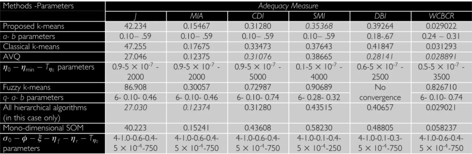
The modified model of thek-means method is executed for different pairs (a,b) from 2 to 10 clusters, where a¼{0.1, 0.11 ,. . ., 0.45} and a + b ¼ {0.54, 0.55, . . ., 0.9}. For each cluster, 1332 different pairs (a, b) are examined. The best results for the six adequacy measures do not refer to the same pair (a, b). From the results of Table 1, it is obvious that the developed k-means is superior to the clas-sical one with the random choice of the input vectors during the centres’ initialisation. For the classical k-means model 100 executions are carried out and the best results for each adequacy measure are recorded. The superiority of the developed model applies in all cases of neurons. A second advantage is the convergence to the same results for the respective pairs (a,b), which can not be achieved using the classical model.

Application of adaptive vector quantisation

The initial value 0, the minimum valuemin and the time

parameter T0 of learning rate must be properly calibrated.

For example in Fig 3 the sensitivity of the ratio of within cluster sum of squares to between cluster variation WCBCR to the ₀ and T0 parameters is presented for 90

experi-ments. The best results of the adequacy measures are not given for the same ₀ and T0, according to the results of

Table 1. The _min value does not practically improve the neural network’s behaviour assuming that it ranges between 10-5_{and 10}-6_.

Application of fuzzy k-means

In the fuzzy k-means method the model is executed for different amount of fuzziness q¼{2, 4, 6}. As an example the WCBCR is presented in Fig 4 for different number of clusters for three cases of q ¼{2, 4, 6}. The best results are given by q¼6, while the respective values forq¼4 is quite similar to those ofq¼6.

Application of mono-dimensional self-organising

maps

Although the mono-dimensional SOM is theoretically well defined, there are several issues that need to be solved for the effective training of SOM. The major problems are:

•

to stop the training process of the optimum SOM. In this case the target is to minimise the index Is

(equation (18)). Generally, it is noticed that the con-vergence is completed after 0.542.0.T0 epochs during fine tuning phase, when T0 has big values (>1000 epochs).

•

the proper calibration of (a) the initial value of the neighbourhood radius 0, (b) the multiplicative factor

between Ts0 (epochs of the rough ordering phase) and T0 (time parameter of learning rate), (c) the Methods -Parameters Adequacy Measure

J MIA CDI SMI DBI WCBCR

Proposed k-means 42.234 0.15467 0.31280 0.35368 0.39264 0.029022 a- bparameters 0.10– .59 0.10– .59 0.10– .59 0.10– .59 0.18-.67 0.24 – 0.31 Classical k-means 47.255 0.17675 0.33473 0.37643 0.41847 0.031293 AVQ 27.046 0.12375 0.31076 0.38665 0.28141 0.028891 0minT0 parameters 0.9-5310 -7 -2000 0.9-5310-7 -2000 0.9-5310-7 -5000 0.1-5310-7 -4000 0.6-5310-7 -2500 0.5-5310-7 -3500 Fuzzy k-means 86.908 0.30057 0.72987 0.90689 No 0.826710 q- a- bparameters 6- 0.10- 0.46 6- 0.10- 0.46 6- 0.10- 0.74 6- 0.28- 0.32 convergence 6- 0.10- 0.74

All hierarchical algorithms (in this case only)

27.030 0.12374 0.31280 0.43515 0.40657 0.029021 Mono-dimensional SOM 40.223 0.15241 0.43608 0.58230 0.48805 0.058237 0 frT0 parameters 4-1.0-0.6-0.4-5310-4_-750 4-1.0-0.6-0.4-5310-4_-750 4-1.0-0.6-0.4-5310-4_-750 4-1.0-0.1-0.4-5310-4_-250 4-1.0-0.1-0.3-5310-4_-750 4-1.0-0.6-0.4-5310-4_-750 Table 1: Comparison of the best clustering models for 4 clusters for the chiller

Fig 3: WCBCRmeasure

of the AVQ method for 4 clusters for the set of 11 training patterns of the chiller with

0¼{0.1, 0.2,. . ., 0.9}, T0¼{500, 1000,. . ., 5000}

Fig 4: WCBCRmeasure of the fuzzy k-means method for 2 to

10 clusters for the set of 11 training patterns of the chiller with q¼2, 4, 6

multiplicative factor between T0 (time parameter of neighbourhood radius) and T0, (d) the proper ini-tial values of the learning rate _r and _f during the rough ordering phase and the fine tuning phase re-spectively. The optimisation process for the mono-dimensional SOM parameters is similar to that one of the application of the adaptive vector quantisation for

0 and T0. The best results for each adequacy

meas-ures are presented in Table 1 for the case of 4 clusters.

•

the initialisation of the weights of the neurons, where the three cases of the theoretical analysis of self-organising maps are examined and the best training behaviour is presented in case (a) (for wki¼0:5,

8k,i).

Application of hierarchical agglomerative algorithms

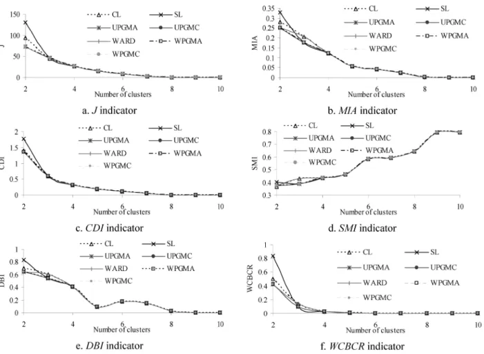
In the case of the seven hierarchical models the best results are given for different models for two and three clusters, while for four clusters or more, all models give the same results, as it is shown in Fig 5. It should be mentioned that there are not any other parameters for calibration, such as maximum number of iterations etc.

Comparison of clustering models for the chiller

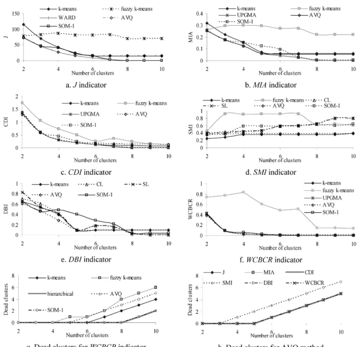
The best results for each clustering method (modified k-means, adaptive vector quantisation, fuzzy k-k-means, self-organised maps and hierarchical methods) are presented in Fig 6. The optimised AVQ and WARD methods present the best behaviour for the mean square error J, the optimised AVQ and the unweighted pair group method average algo-rithm (UPGMA) for the MIA, the optimised AVQ and the modified k-means for the CDI, DBI and WCBCR, the modified k-means for the SMI. All measures (except DBI) show an improved performance, as the number of clusters increases.

The number of dead clusters for the WCBCR indicator for all clustering techniques and for all adequacy measures for AVQ method are shown in Fig 6g and 6h respectively. Here, it is not obvious which measure is the best one because of the extremely small set of training patterns. However, taking into consideration the results3,10_{and noting}

that the basic theoretical advantage of the WCBCR measure is that it combines the distances of the input vectors from the representative clusters and the distances between clus-ters (covering also the J and CDI characteristics), the appli-cation of WCBCR is proposed.

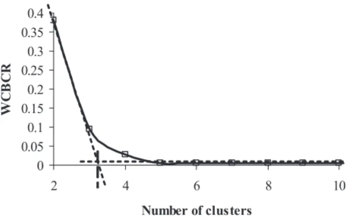
Observing Fig 6f, the improvement of the WCBCR is significant up to 4 clusters. After this value, the behaviour

Fig 5: Adequacy measures of the 7 hierarchical clustering algorithms for 2 to 10 clusters for the set of 11 training patterns of the chiller

Fig 6: Adequacy measures and dead clusters of each clustering method for 2 to 10 clusters for the set of 11 training patterns of the chiller Type Number of clusters Population of the Best clustering Date representative cluster

technique November 1997 January 1998

20 21 22 23 24 25 26 27 1 2 3 a 4 7 AVQ 2nd ₃rd ₃rd ₁st ₄th ₄th ₄th ₄th ₄th ₄th ₄th b 3 9 CL - UPGMC 2nd ₁st ₁st ₁st ₁st ₁st ₁st ₁st ₃rd ₁st ₁st c 4 7 k-means 4th ₃rd ₄th ₄th ₄th ₄th ₄th ₄th ₂nd ₁st ₁st d 4 6 UPGMC 4th ₃rd ₄th ₄th ₁st ₁st ₁st ₁st ₁st ₂nd ₁st e 3 8 All hierarchical 1st ₂nd ₁st ₁st ₁st ₁st ₁st ₃rd ₁st ₂nd ₁st f 4 8 k-means 1st ₂nd ₁st ₁st ₁st ₁st ₁st ₁st ₄th ₃rd ₁st Table 2: Results of the methodology for 6 electrical consumers of HN MEKO Type frigates, where type ‘a’ is the chiller, type ‘b’ the HP compressor FWD/AFT, type ‘c’ the refrigeration plant, type ‘d’ the LP compressor FWD/AFT, type ‘e’ the sanitary plant, type ‘f’ the boiler respectively

of the adequacy measure is gradually stabilised. It can also be estimated graphically, using the ‘knee-rule’, of which gives values between 3 to 4 clusters (see Fig 7). In Fig 8 the typical daily chronological ON/OFF load curves for the

chiller are presented using the AVQ method with the best WCBCR measure for 4 clusters.

The training time for the methods under study has the ratio 0.05:1:22:24:36 (hierarchical: proposed k-means: opti-mised adaptive vector quantisation: mono-dimensional self-organising map: fuzzy k-means for q¼6). Therefore, the k-means, AVQ and hierarchical models have been selected.

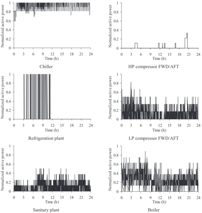
Application of the clustering models for the other

electric consumers

The same methodology is applied to the other five electric consumers. In Table 2, the total number of clusters, the population of the representative cluster, the respective clus-tering technique and the clusters calendar are registered for each consumer. It is obvious that the modified k-means, the AVQ and the hierarchical (especially UPGMC) clustering techniques compete each other, while the fuzzy k-means and self-organising map techniques have poor results in this kind of classification. It is reminded that the representative

Fig 7: WCBCRmeasure of theAVQmodel for 2 to 10 clusters

for the set of 11 training patterns of the chiller and the use of the tangents for the estimation of the knee

Fig 8: The typical daily chronological ON/OFF load curves for the chiller for four clusters using AVQ method

cluster is the most populated one. In Fig 9, the respective representative typical load diagrams are presented.

CONCLUSIONS

This paper presents an efficient pattern recognition method-ology for the study of the load demand behaviour of elec-trical consumers of ships. Unsupervised clustering methods can be applied, such as the k-means, adaptive vector quanti-sation (AVQ), fuzzy k-means, mono-dimensional self-orga-nising maps (SOM) and hierarchical methods. The performance of these methods is evaluated by six adequacy measures: mean square error, mean index adequacy, cluster-ing dispersion indicator, similarity matrix indicator, Davies-Bouldin indicator, the ratio of within cluster sum of squares to between cluster variation. Finally, the representative daily load diagrams along with the respective populations per each consumer are calculated. This information is valuable for ship engineers, because it facilitates the formalisation of

the electrical consumer’s load behaviour, the design, the operation and the reliability of the ship’s power system and the improvement of the operation of the automatic battle management system for a battleship.

From the respective application for six consumers of HN MEKO type frigates electric system for a small dataset (only 11 training sets), it is concluded that three to four clusters suffice for the satisfactory description of the daily load curves of each consumer. It is also concluded that the optimal clustering technique is the modified k-means, the AVQ and the hierarchical clustering techniques, while the optimal adequacy measure is the ratio of within cluster sum of squares to between cluster variation.

These results surely depend on the population of the data set, the ship operating mode (‘anchor’, ‘shore’, ‘at sea’, ‘general quarter’) and the load curve’s time interval (in this case study, it was a day). In the future, it should be investigated in larger datasets for longer study periods with different time intervals (from few hours to days).

REFERENCES

1. Hatzilau IK, Perros S, Karamolegos G, Galanis K, Dalakos A, Anastasopoulos K, Kavousanos A and Eno-tiadis X. 1998. Load estimation of MEKO Class frigates – Field measurements, results. Proceedings of the Inter-national Conference on The Naval Technology for the 21st _{Century, pp225-232, 29-30 June 1998, Pireaus,}

Greece.

2. Chicco G, Napoli R, Postolache P, Scutariu M and Toader C. 2003, Customer characterisation for improving the tariff offer, IEEE Transactions Power Systems, 18-1: 381-387.

3. Tsekouras GJ, Hatziargyriou ND and Dialynas EN. 2007. Two-stage pattern recognition of load curves for classification of electricity customers. IEEE Transactions Power Systems, 22-3: 1120-1128.

4. Gerbec D, Gasperic S, Smon I and Gubina F. 2005.

Allocation of the load profiles to consumers using probabil-istic neural networks. IEEE Transactions Power Systems, Vol 20-2: 548-555.

5. Chicco G, Napoli R and Piglione F. 2006. Compari-sons among clustering techniques for electricity customer classification. IEEE Transactions Power Systems, Vol 21-2: 933-940.

6. Theodoridis S and Koutroumbas K. 1999. Pattern Recognition, 1st_{ed. New York: Academic Press.}

7. Figueiredo V, Rodrigues F, Vale Z, Gouveia JB. 2005.

An electric energy consumer characterization framework based on data mining techniques. IEEE Trans. Power Syst, Vol. 20-2: 596-602.

8. Petrescu M, Scutariu M. 2002.Load diagram charac-terisation by means of wavelet packet transformation. 2nd

Balkan Conference, Belgrade, Yugoslavia, June 2002. 9. Chen C S, Hwang J C, Huang C W. 1997.Application of load survey systems to proper tariff design. IEEE Trans. Power Syst,Vol. 12-3: 1746-1751.

10. Tsekouras GJ, Kotoulas PB, Tsirekis CD, Dialynas EN, Hatziargyriou ND. 2008.A pattern recognition method-ology for evaluation of load profiles and typical days of large electricity customers. Electrical Power Systems Re-search, Vol. 78-9: 1494-1510.

11. Hatzilau IK, Tsekouras GJ, Prousalidis J, Gyparis IK. On electric load characterization and categorization in ship electric installations. INEC-2008, 1-3 April 2008, Hamburg, Germany.

12. Duda RO, Hart PE, Stork DG. 2001. Pattern Classi-fication. 1st edition, A Wiley-Interscience Publication.

13. Haykin S. 1994. Neural networks: A comprehensive foundation. 2nd Edition, Prentice Hall, NJ, 1994.

14. Kohonen T. 1989. Self–organization and associative memory. 2nd Edition, Springer-Verlag, NY.

15. SOM Toolbox for MATLAB 5. 2000. Helsinki, Fin-land: Helsinki Univ. Technology.

16. Chicco G, Napoli R, Piglione F, Scutariu M, Post-olache P, Toader C. 2002. Options to classify electricity customers. Med Power 2002, 4-6 November, Athens, Greece

17. Hand D, Manilla H, Smyth P. 2001. Principles of data mining. The MIT Press, Cambridge, Massachusetts, London, England.