Analysing the impact of decoupling at a regional level in Ireland:
A farm level dynamic linear programming approach
Shailesh Shrestha and Thia Hennessy
Rural Economy Research Centre, Teagasc, Athenry, Co Galway, Ireland Contact email: [email protected]
Contributed paper prepared for presentation at the Ineternational Association of Agricultural Economists Conferece, Gold Coast, Australia, August 12-18, 2006
Copyright 2006 by Shailesh Shrestha and Thia Hennessy. All rights reserved. Readers may make verbatim copies of this document for non-commercial purposes by any means, provided that this copyright notice appears on all such copies.
Introduction
In Ireland, all direct payments made to farmers were completely decoupled from production in January 2005. A single payment is paid to the farmers based on payments they received in a historical reference period. There have been earlier studies on possible impacts of decoupling on Irish farms (Breen et al., 2005; Breen and Hennessy 2003). The results from these studies showed that decoupling was likely to accelerate the pace of structural change in Irish farming for instance, thirty-two percent of dairy farms were projected to exist the sector and ten percent of cattle farms are likely to become entitlement farmers that is using their land to claim the decoupled payment but not actually produce any tangible products. However, these studies took a generalized view of farms in Ireland and didn’t address the regional differentiation that may arise as a result of decoupling. It is fair to say that the impact of a policy change may be different at different regional levels. Any possible changes especially land use and milk quota structures are highly depended on geographical location of farms. For example, milk quota trade in Ireland is restricted within a region or a co-operative. This paper describes a methodology that was used in a study to determine impacts of decoupling of farm payments at the regional level in Ireland and provides an example with the results from one of the regions.
Methodology
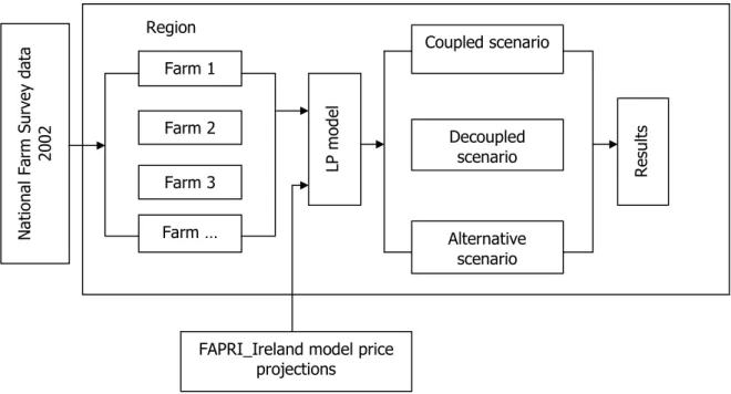
The methodology outlined in this paper is shown in figure 1. The first step of the methodology involves a collation of farm level data on physical entities of a farm,
such as farm size and animal numbers; farming activities which takes place on farm such as dairying activities, beef activities; and farm accounting details such as input costs, revenues received. The study used Irish National Farm Survey Data from 2002 (NFS), a part of Farm Accountancy Data Network (FADN), which is a survey to collect accountancy data carried out by the member states of the European Union.
The second step of the methodology involves a selection of representative farms and separation of farms into groups with similar characteristics. Clustering techniques namely hierarchical, non-hierarchical, iterative partitioning and factor analytic techniques are available for this purpose.
Figure 1: A schematic diagram of the methodology
A number of variables such as total farm area, gross margins, animal number, milk yield, labour units, productivity (per hectare area and per labour unit) are used to group farms into clusters. The identification of farm variables to include in the cluster analysis is largely arbitrary but one should take care to use variables which are directly related to the criteria on which grouping is based. For example, if dairy farms are to be clustered together, the most obvious variables to be chosen are dairy numbers, milk yield, total milk production and milk quota number. Cluster analysis measures the degree of similarity between two or more unrelated objects in terms of the number of variables they possess. This method enables the formation of groups of objects with homogenous characteristics within the groups and heterogeneous characteristics between the groups (Everitt, 1993). The clusters in this study were formed using an agglomerative hierarchical cluster technique. In
this technique, all farms are placed in different groups at the beginning and after that, farms closer to each other are grouped together in a stepwise fashion. It follows then that all farms should be placed in one single group at the end. Hierarchical cluster analysis has been used to form groups in different farm level analyses (Rey and Das, 1997; Kirke and Moss, 1987; Solano et al., 2001). Within the hierarchical method, there are a number of techniques to measure the distance between to variables and link them if they are similar. The Squared Euclidean Distance Method was used in this study to measure distance between variables and the Ward method was used to link similar variables. These methods are useful when there are multi-dimensional variables such as farm size and milk yield (Solano et al., 2001). Once the farms were clustered in different groups, average values from each farm group were taken and used as inputs to the base year 2002 in the study.
The third step of the methodology involves in developing an optimising mathematical programming model which maximises an objective function within a number of limiting constraints. There are a number of optimising models such as Linear Programming, Positive Mathematical Programming, Non Linear Programming which can be used for this purpose. This study used a farm level dynamic linear programming model to maximise regional gross margin; first, under a baseline scenario where payments were coupled with production and second, under an alternative scenario where payments were decoupled and a single farm payment was introduced. A brief description of the model is given below to explain how it was used.
The model used a time frame of 15 years and had an objective function to maximise farm gross margins within a set of constraints. It consisted of all possible farm enterprises (i.e., dairy, beef, sheep and tillage) for each type of farms present in a region. However, all the farming activities in individual farms were independent to each other and a farm could not start a new enterprise without investing a starting capital if that enterprise did not exist in the base year i.e., year 1 of the model run. The only link between different farms within a region was through land and milk quota transfer. If there was no transfer of these two components between the farms, the objective function of the model was the cumulative gross margins of individual farm types within that region. In the model, farmland was comprised of grassland, permanent pasture and arable land (in the case of tillage farms). Grassland was further divided into grazing land and silage land with silage land restricted to a maximum of 50% of total grassland. Livestock were constrained under a fixed stocking rate (as recorded in the base year) over grazing land. Land transfer was constrained in a way that a farm could only lease in land if another farm was leasing out land. At the equilibrium, total rented in land was equal to total leased out land. Grassland could not be converted to arable land, however, arable land was allowed to transfer to grassland or could be leased out.
Livestock numbers present on the farm type was first initialised in the base year according to the survey data. In subsequent years, the number of livestock in year Y was dependent on the number of livestock in period Y-1 plus purchased animals less animals that had been sold. Livestock replacements were reared from the herd or alternatively may be purchased. Dairy animals were culled every five years,
whereas calves, beef, lamb and ewe could be sold whenever it was most profitable. Total feed used on the farm depended on the energy, protein and dry matter requirements of each animal and the content in each feed type. Feed requirements were based on growth, maintenance, pregnancy and production levels. There were three types of feed available; fresh grass, grass silage and concentrate feed in this study. At least a minimum level of grass silage and concentrate feed based on the survey data was maintained on a farm.
Milk production linked different types of dairy farms in a region by allowing milk quota transfer between dairy farms. Dairy farms had a fixed quantity of owned quota as recorded in the base year. Total milk production was a function of cow numbers and was equal to quota owned in the base year. However, flexibility in milk production was allowed in the model through leasing and renting of milk quota. A farm could rent in quota only if leased out quota was available from another dairy farm within the same region.
The model did not include a crop rotation constraint because tillage farming was not an important activity in Ireland. In this model, the crop choice set consisted only of the crops grown in the base year was considered. Set aside land was constrained between 5% (obligatory level) and 25% (voluntary level) of the total arable land. Crop variable costs including fertiliser costs, seeds costs and insecticides costs, were taken from published data. All machinery operations required for arable crops were contracted in and used as contract costs in the model. There were two types of labour present on farms; family and hired labour. Labour was used in livestock
enterprises only as arable activities had been contracted in. Total labour used on farm was a function of the labour requirements by each enterprise.
Prices of different farm commodities and costs of different farm inputs such as fertiliser and seed costs, transport costs etc were the averaged values in each farm group generated in the cluster analysis. As the model used in this study was a dynamic model, these prices and costs were required to be projected over 15 years. Price indices from the FAPRI-Ireland model1 were used in the study. The FAPRI_Ireland model is a partial equilibrium model which econometrically estimates prices of different agricultural commodities over a length of time taking account of the world and EU prices. Two sets of price projection were generated by the FAPRI_Ireland model; one under the baseline scenario which was a continuation of AGENDA 2000 policies and the second, under a decoupled scenario, which was the 2003 MTR of the CAP. The current study used the price and cost projections emanating from the FAPRI-Ireland baseline and MTR scenarios and applies these projections to the farm level data.
The final step of the analysis involved in running the model for the baseline and the MTR scenarios. The Baseline scenario used the farm level data taken from each farm groups and the set of projected prices for the baseline scenario. The farm data used in that scenario included all farm payments received by a farm in 2002. For the MTR scenario, all the payments received by a farm in 2002 were summed up and paid to the farm as a single payment. The payment was linked to land and was paid
1
FAPRI-Ireland model is a part of FAPRI model which was established in the Universities of Iowa and Missouri in 1984 and uses partial equilibrium models of agricultural markets to show the effects of policy change on commodity prices, volumes of production and trade and many other economic indicators. For a description of the Irish model see Binfield et al (2003)
on a per hectare basis and therefore claiming of payments was a land using activity in the model. The single farm payment was calculated on per hectare of farmland basis and then added to the annual margins. This scenario used the set of price projection for the MTR scenario. Besides payments and prices, values for all other farm variables and parameters remained same as under the baseline scenario so that the difference between the results in these two scenarios could be concluded as the impact of decoupling. The results of the model for the Border region are described below.
Results
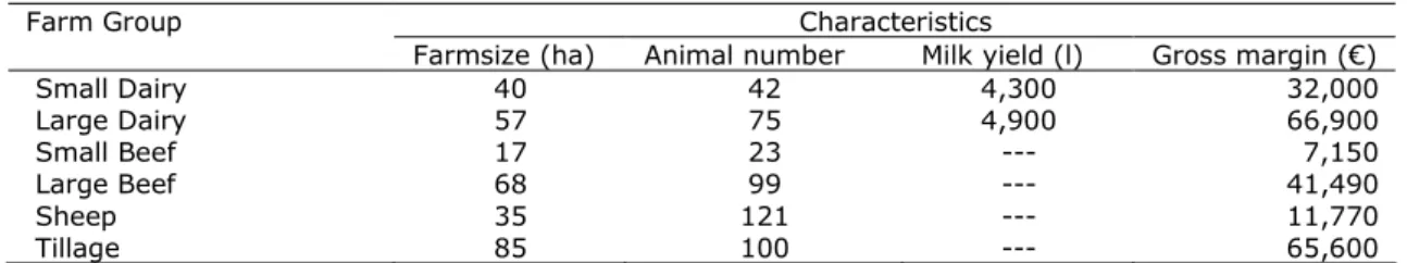
The Border region consists of 6 counties; Louth, Leitrim, Sligo, Donegal, Cavan and Monaghan. As mentioned earlier, farm level data for the farms in the region are drawn from the 2002 Irish National Farm Survey data (NFS). The farm survey, surveys a stratified random sample of approximately 200 farms each year in this region. Within the survey, farms are already separated into 4 different farming systems; dairy, beef, sheep and tillage, according to the contribution of an enterprise to the farm gross margin. The cluster analysis resulted in 10 farm groups in this region; three dairy groups, five beef groups and one sheep group and one tillage group. The characteristics of major farm groups in the region are as shown in Table 1.
Table 1: Farm groups in Region 1 and their characteristics
Validation
Validation is one of the important aspects in modelling work. Model results need to be validated to see if model behaves as been expected. In this study, the model results for the annual margins for each farm in the base year were compared with the gross margin of each farm groups as recorded in the NFS. Figure 2 shows a comparison between the actual and projected margins for 2002.
Figure 2: The percentage change in the model gross margins compared to the NFS gross margins in selected farm groups
The results showed that the model was over-estimating farm margin in dairy farms whereas underestimating in all other farm groups especially in tillage farms where model results were 37% lower than the actual figures. This difference in gross margin could be due to the method of calculation employed in the model. For example, the gross margin in the model did not include special payments such as REPS, DACAS but they were included in the survey data. The difference in the gross margin was much smaller when these payments are included in the model.
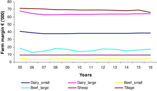
Baseline scenario
In the baseline scenario, the annual margins of all farms groups remained almost constant over 12 years projection period after year 2005 (Figure 3). The initial changes in farm margins were due to adjustment of animals on farms. Sheep farms and Small beef farms had the lowest annual margin whereas tillage farms and large dairy farms had the largest annual farm margins in this region.
Figure 3: Gross margin in selected farm types under baseline scenario
Decoupled scenario
Under the decoupled scenario, the gross margin on small dairy farm was projected to decrease by 6.5% compared to the margin with coupled farm payments. The small dairy farms were less efficient with lower yielding cows and higher input costs. Furthermore, they also received lower milk and having a small number of beef animals in the base year, received a smaller single farm payment. It was projected that 14% of grassland move away from these farms and it was optimal for these farms to decrease the number of dairy animals on the farm. In contrast, large dairy farms are projected to slightly increase in herd size under the decoupled scenario. There was a projection of 4% increase in farm gross margin on these farms. The results therefore suggested that decoupling was likely to result in the greater concentration of milk production on to fewer farms in the Border region. Figure 4 shows that after decoupling, the margins in dairy farms are projected to decrease by 10% over 12 years time period. Much of this decrease is due to a decrease in milk price (-10%) and increase in livestock variable costs (+20%) over the same period.
Gross margins were projected to decrease in beef farms after decoupling of the payments. The margins in the decoupled scenario were much lower compared to the margins under the baseline scenario. This was because beef numbers in these farms under the decoupled scenario were lower than the baseline scenario as the payments were based on the number of animals in the base year only. Once the payments were decoupled from production, beef animals were less profitable and it
was optimal for the farms to decrease animal numbers to reduce input costs. However, beef farms especially large beef farms showed signs of recovery as beef prices begin to increase again after the initial decoupling shock. At this stage, the beef farms in the model did not change to other enterprise because of the investment constraints on changing enterprise. To change to dairy, there was a starting cost constraint where as sheep wasn’t profitable enough for the change. Figure 4: Gross margins in the selected farm types under decoupled scenario
There was an increase in annual margins for the tillage farms in the decoupled scenario relative to the baseline scenario. Tillage farms in the region continued spring wheat production which remained profitable to some extent after decoupling. However, when the projected wheat price dropped beyond profitability (after year 2012), all arable area is transferred to grassland and arable farms moved into sheep farming. Arable farms benefit financially from decoupling because they retained their payments and reducing crop variable costs by decreasing crop production. They also benefited from an increase in the sheep price.
The farm margins in sheep farms were projected to increase slightly over the years in the decoupled compared to the baseline scenario over the years which was due to an increase in sheep numbers responding to a projection of higher sheep price.
Conclusion
The impact of a policy change differs widely between farm types and farm location. A farm level analysis of policy change at a regional level provides an opportunity to compare the impact of a policy change on farms between different regions. Furthermore, if the study regions, such as NUTS regions, are internationally recognised then it is possible to compare the effect of a EU wide policy change in a region of one country with regions in other countries. The example provided in this paper, although just for one region in Ireland, can be compared to the results for other regions in Ireland as well as other European regions.
Reference
Binfield, J., T. Donnellan, K. Hanrahan and P. Westhoff, 2003. The Luxembourg CAP Reform Agreement: Implication for EU and Irish Agriculture. The Luxembourg CAP Reform Agreement: Analysis of the Impact on EU and Irish Agriculture, pp. 1-69, Teagasc, Dublin.
Breen, J. P., and T. C. Hennessy, 2003. The impact of the MTR and the WTO reform on Irish farms. Outlook 2003, Medium Term Analyisi for the Agri-Food Sector, Teagasc, Dublin, 78-92.
Breen, J. P., T. C. Hennessy, and F. S. Thorne, 2005. The effect of decoupling on the decision to produce: An Irish case study. Food Policy 30: 129-144.
Everitt, B., 1993. Cluster analysis (3rd Ed.). Edward Arnold, London.
Kirke, A. W. and J. E. Moss. 1987. A linear programming study of family-run dairy farms in Northern Ireland. Journal of Agricultural Economics 38:257-269.
Rey, B. and S. M. Das. 1997. A system analysis of inter-annual changes in the pattern of sheep flock productivity in Tanzanian livestock research centres. Agricultural Systems. 53: 175-189.
Solano, C., H. Leon, E. Perez, and M. Herrero. 2001. Characterising objectives profiles of Costa Rican dairy farmers. Agricultural Systems. 67: 153-179.
Figure 1: A schematic diagram of the methodology N a ti o n a l F a rm S u rv e y d a ta 2 0 0 2 Farm 1 Farm 2 Farm 3 Farm … Region L P m o d e l Coupled scenario Decoupled scenario Alternative scenario R e su lt s
FAPRI_Ireland model price projections
Table 1: Farm groups in Region 1 and their characteristics
Farm Group Characteristics
Farmsize (ha) Animal number Milk yield (l) Gross margin (€)
Small Dairy 40 42 4,300 32,000 Large Dairy 57 75 4,900 66,900 Small Beef 17 23 --- 7,150 Large Beef 68 99 --- 41,490 Sheep 35 121 --- 11,770 Tillage 85 100 --- 65,600 0 20 40 60 80
Dairy_small Dairy_large Beef_small Beef_large Sheep Tillage
Farm types € ( '0 0 0 ) Model NFS '02
Figure 2: The percentage change in the model gross margins compared to the NFS gross margins in selected farm groups
0 10 20 30 40 50 60 70 80 05 06 07 08 09 10 11 12 13 14 15 16 Years F a rm m a rg in € ( '0 0 0 )
Dairy_small Dairy_large Beef_small
Beef_large Sheep Tillage
Figure 3: Gross margin in selected farm types under baseline scenario
0 10 20 30 40 50 60 70 05 06 07 08 09 10 11 12 13 14 15 16 Years F a rm m a rg in s € ( '0 0 0 )
Dairy_small Dairy_large Beef_small
Beef_large Sheep Tillage