BestPeer++: A Peer-to-Peer based Large-scale
Data Processing Platform
Gang Chen
#†1, Tianlei Hu
#†2, Dawei Jiang
‡3, Peng Lu
‡4, Kian-Lee Tan
‡5, Hoang Tam Vo
‡6, Sai Wu
∗‡7 #NetEase.com Inc., †Zhejiang University1,2{cg, htl}@cs.zju.edu.cn
∗BestPeer Pte. Ltd., ‡National University of Singapore 3,4,5,6,7{
jiangdw, lupeng, tankl, voht, wusai}@comp.nus.edu.sg
Abstract— The corporate network is often used for sharing information among the participating companies and facilitating collaboration in a certain industry sector where companies share a common interest. It can effectively help the companies to reduce their operational costs and increase the revenues. However, the inter-company data sharing and processing poses unique challenges to such a data management system including scalability, performance, throughput, and security. In this paper, we present BestPeer++, a system which delivers elastic data sharing services for corporate network applications in the cloud based on BestPeer – a peer-to-peer (P2P) based data management platform.
By integrating cloud computing, database, and P2P tech-nologies into one system, BestPeer++ provides an economical, flexible and scalable platform for corporate network applications and delivers data sharing services to participants based on the widely accepted pay-as-you-go business model. We evaluate BestPeer++ on Amazon EC2 Cloud platform. The benchmarking results show that BestPeer++ outperforms HadoopDB, a recently proposed large-scale data processing system, in performance when both systems are employed to handle typical corporate network workloads. The benchmarking results also demonstrate that BestPeer++ achieves near linear scalability for throughput with respect to the number of peer nodes.
I. INTRODUCTION
Companies of the same industry sector are often connected into a corporate network for collaboration purposes. Each company maintains its own site and selectively shares a portion of its business data with the others. Examples of such corporate networks include supply chain networks where organizations such as suppliers, manufacturers, and retailers collaborate with each other to achieve their very own business goals including planning production-line, making acquisition strategies and choosing marketing solutions.
From a technical perspective, the key for the success of a
corporate network is choosing the rightdata sharingplatform,
a system which enables the shared data (stored and maintained by different companies) network-wide visible and supports efficient analytical queries over those data. Traditionally, data sharing is achieved by building a centralized data warehouse, which periodically extracts data from the internal production systems (e.g., ERP) of each company for subsequent querying. Unfortunately, such a warehousing solution has some deficien-cies in real deployment.
First, the corporate network needs to scale up to support thousands of participants, while the installation of a large-scale centralized data warehouse system entails nontrivial costs including huge hardware/software investments (a.k.a Total Cost of Ownership) and high maintenance cost (a.k.a Total Cost of Operations) [12]. In the real world, most companies are not keen to invest heavily on additional information systems until they can clearly see the potential return on investment (ROI) [16]. Second, companies want to fully customize the access control policy to determine which business partners can see which part of their shared data. Unfortunately, most of the data warehouse solutions fail to offer such flexibilities. Finally, to maximize the revenues, companies often dynamically adjust their business process and may change their business partners. Therefore, the participants may join and leave the corporate networks at will. The data warehouse solution has not been designed to handle such dynamicity.
To address the aforementioned problems, this paper presents BestPeer++, a cloud enabled data sharing platform designed for corporate network applications. By integrating cloud com-puting, database, and peer-to-peer (P2P) technologies, Best-Peer++ achieves its query processing efficiency and is a promising approach for corporate network applications, with the following distinguished features.
• BestPeer++ is deployed as a service in the cloud. To
form a corporate network, companies simply register their sites with the BestPeer++ service provider, launch BestPeer++ instances in the cloud and finally export data to those instances for sharing. BestPeer++ adopts the pay-as-you-go business model popularized by cloud computing [5]. The total cost of ownership is therefore substantially reduced since companies do not have to buy any hardware/software in advance. Instead, they pay for what they use in terms of BestPeer++ instance’s hours and storage capacity. The BestPeer++ service provider elastically scales up the running instances and makes them always available. Therefore, companies can use the ROI driven approach to progressively invest on the data sharing system.
• BestPeer++ extends the role-based access control for the
Through a web console interface, companies can easily configure their access control policies and prevent unde-sired business partners to access their shared data.
• BestPeer++ employs P2P technology to retrieve data
between business partners. BestPeer++ instances are or-ganized as a structured P2P overlay network named BATON [9]. The data are indexed by the table name, column name and data range for efficient retrieval.
• BestPeer++ employs a hybrid design for achieving high
performance query processing. The major workload of a corporate network is simple, low-overhead queries. Such queries typically only involve querying a very small number of business partners and can be processed in short time. BestPeer++ is mainly optimized for these queries. For infrequent time-consuming analytical tasks, we provide an interface for exporting the data from BestPeer++ to Hadoop and allow users to analyze those data using MapReduce.
In summary, the main contribution of this paper is the design of BestPeer++ system that provides economical, flexible and scalable solutions for corporate network applications. We demonstrate the efficiency of BestPeer++ by benchmarking BestPeer++ against HadoopDB [2], a recently proposed large-scale data processing system, over a set of queries designed for data sharing applications. The results show that for sim-ple, low-overhead queries, the performance of BestPeer++ is significantly better than HadoopDB.
The rest of the paper is organized as follows. Section II presents the overview of BestPeer++ system. We subsequently describe the design of BestPeer++ core components, including the bootstrap peer in Section III and the normal peer in Section IV. The pay-as-you-go query processing strategy adopted in BestPeer++ is presented in Section V. Section VI evaluates the performance of BestPeer++ in terms of efficiency and through-put. Related work are presented in Section VII, followed by conclusion in Section VIII.
II. OVERVIEW OF THEBESTPEER++ SYSTEM
In this section, we first describe the evolution of BestPeer platform from its early stage as an unstructured P2P query processing system to BestPeer++, an elastic data sharing services in the cloud. We then present the design and overall architecture of BestPeer++.
BestPeer1 data management platform. While traditional
P2P network has not been designed for enterprise applications, the ultimate goal of BestPeer is to bring the state-of-art database techniques into P2P systems. In its early stage, Best-Peer employs unstructured network and information retrieval technique to match columns of different tables automatically [11]. After defining the mapping functions, queries can be sent to different nodes for processing. In its second stage, BestPeer introduces a series of techniques for improving query performance and result quality to enhance its suitability for
1http://www.comp.nus.edu.sg/∼bestpeer/
corporate network applications. In particular, BestPeer pro-vides efficient distributed search services with a balanced tree structured overlay network (BATON [9]) and partial indexing scheme [20] for reducing the index size. Moreover, BestPeer develops adaptive join query processing [21] and distributed online aggregation [19] techniques to provide efficient query processing.
BestPeer++, a cloud enabled evolution of BestPeer.Now
in the last stage of its evolution, BestPeer++ is enhanced with distributed access control, multiple types of indexes, and pay-as-you-go query processing for delivering elastic data sharing services in the cloud. The software components of
BestPeer++ are separated into two parts: core and adapter.
The core contains all the data sharing functionalities and is designed to be platform independent. The adapter contains one abstract adapter which defines the elastic infrastructure service interface and a set of concrete adapter components which implement such an interface through APIs provided by specific cloud service providers (e.g., Amazon). We adopt this “two-level” design to achieve portability. With appropriate adapters, BestPeer++ can be ported to any cloud environments (public and private) or even non-cloud environment (e.g., on-premise data center). Currently, we have implemented an adapter for Amazon cloud platform. In what follows, we first present this adapter and then describe the core components.
A. Amazon Cloud Adapter
The key idea of BestPeer++ is to use dedicated database servers to store data for each business and organize those database servers through P2P network for data sharing. The Amazon Cloud Adapter provides an elastic hardware in-frastructure for BestPeer++ to operate on by using Ama-zon Cloud services. The infrastructure service that AmaAma-zon Cloud Adapter delivers includes launching/terminating dedi-cated MySQL database servers and monitoring/backup/auto-scaling those servers.
We use Amazon EC2 service to provision the database server. Each time a new business joins the BestPeer++ net-work, we launch a dedicated EC2 virtual server for that busi-ness. The newly launched virtual server (called a BestPeer++ instance) runs a dedicated MySQL database software and the BestPeer++ software. The BestPeer++ instance is placed in a separate network security group (i.e., a VPN) to prevent invalid data access. Users can only use BestPeer++ software to submit queries to the network.
We use Amazon Relational Data Service (RDS) to back
up and scale each BestPeer++ instance2. The whole MySQL
database is backed up to Amazon’s reliable EBS storage devices in a four minute window. There will be no service interrupt during the process since the backup operation is performed asynchronously. The scaling scheme consists of two dimensions: processing and storage. The two dimensions can be independently scaled up. Initially, each BestPeer++ instance 2Actually, the server provisioning is also through RDS service which internally calls EC2 service to launch new servers.
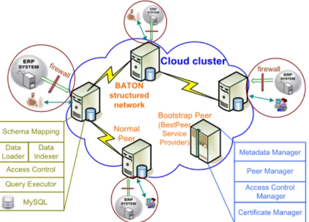
BATON structured network Cloud cluster Normal Peer (BestPeer Service Provider) Metadata Manager Peer Manager Access Control Manager Certificate Manager Bootstrap Peer fire wall Data Loader Schema Mapping MySQL Query Executor Data Indexer Access Control firewall
Fig. 1. The BestPeer++ network deployed on Amazon Cloud offering
is launched as am1.smallEC2 instance (1 virtual core, 1.7
GB memory) with 5GB storage space. If the workload grows, the business can scale up the processing and the storage. There is no limitation on the resources used.
Finally, the Amazon Cloud Adapter also provides automatic fail-over service. In a BestPeer++ network, a special Best-Peer++ instance (called bootstrap peer) monitors the health of all other BestPeer++ instances, by querying the Amazon CloudWatch service. If the bootstrap peer finds another in-stance fails to respond (e.g., crashed), it calls Amazon Cloud Adapter to perform fail-over for that instance. The details of fail-over are presented in Section III.
B. The BestPeer++ Core
The BestPeer++ core contains all platform-independent logic, including query processing and P2P overlay. It runs on top of adapter and consists of two software components:
bootstrap peer and normal peer. A BestPeer++ network can only have a single bootstrap peer instance which is always launched and maintained by the BestPeer++ service provider and a set of normal peer instances. The architecture is depicted in Figure 1. This section briefly describes the functionalities of these two peers. Individual components and data flows inside these peers are presented in the subsequent sections.
The bootstrap peer is the entry point of the whole network. It has several responsibilities. First, the bootstrap peer serves for various administration purposes, including monitoring and managing normal peers registration and also scheduling vari-ous network management events. Second, the bootstrap peer acts as a central repository for storing meta data of corpo-rate network applications, including shared global schema, participant normal peer list, and role definitions. In addition, BestPeer++ employs the standard PKI encryption scheme to encrypt/decrypt data transmitted between normal peers in order to further increase the security of the system. Thus, the bootstrap peer also acts as a Certificate Authority (CA) center for certifying the identities of normal peers.
Normal peers are the BestPeer++ instances launched by businesses. Each normal peer is owned and managed by a unique business and serves the data retrieval requests issued from the users of the owning business. To meet the high
throughput requirement, BestPeer++ does not rely on a cen-tralized server to locate which normal peer hold which tables. Instead, the normal peers are organized as a balanced tree peer-to-peer overlay based on BATON [9]. The query processing is, thus, performed in entirely a distributed manner. Details of query processing is presented in Section V.
III. BOOTSTRAPPEER
The bootstrap peer is run by the BestPeer++ service provider, and its main functionality is to manage the Best-Peer++ network. This section presents how bootstrap peer performs various administrative tasks.
A. Managing Normal Peer Join/Departure
Each normal peer which wants to join an existing corporate network must first connect to the bootstrap peer. If the join request is permitted by the service provider, the bootstrap peer will put the newly joined peer into the peer list of the corporate network. At the same time, the joined peer will receive the corporate network information including the current participants, global schema, role definitions, and an issued certificate. When the normal peer needs to leave the network, it will also notify the bootstrap peer. The bootstrap peer will put the departure peer on the black list and mark the certificate of the departing peer invalid. Then, the bootstrap peer will release all resources allocated for the departing peer back to the cloud and finally remove the departing peer from the peer list.
B. Auto Fail-over and Auto-Scaling
In addition to managing peer join and peer departure, the bootstrap peer is also responsible for monitoring the health of normal peers and scheduling fail-over and auto-scaling events. The bootstrap periodically collects performance metrics of each normal peer. If some peers are malfunctioned or crashed, the bootstrap peer will trigger an automatic fail-over event for each failed normal peer. The automatic fail-over is performed by first launching a new instance from the cloud. Then, the bootstrap peer asks the newly launched instance to perform database recovery from the latest database backup stored in Amazon EBS. Finally, the failed peer is put into the blacklist. On the other hand, if any normal peer is overloaded (e.g., CPU is over-utilized or free storage space is low), the bootstrap peer triggers an auto-scaling event to either upgrade the normal peer to a larger instance or allocate more storage spaces. At the end of each maintenance epoch, the bootstrap releases the resources in the blacklist and notifies the changes to all participants.
IV. NORMALPEER
The normal peer software consists of five components: schema mapping, data loader, data indexer, access control, and query executor. We present the first four components in this section. Query processing in BestPeer++ will be presented in the next section.
As shown in Figure 2, there are two data flows inside the normal peer: an offline data flow and an online data flow.
Local Business Data Management System BestPeer Node firewall data exporting BootStrap schema mapping
(a)Offline Data Flow
BestPeer Node (Query Processor)
BootStrap shuffled data
BestPeer Node BestPeer Node BestPeer Node ... metadata shuffled data shuffled data user
(b)Online Data Flow
Fig. 2. Data Flow in BestPeer++
In the offline data flow, the data are extracted periodically by a data loader from the business production system to the normal peer instance. In particular, the data loader extracts the data from the business production system, transforms the data format from its local schema to the shared global schema of the corporate network according to the schema mapping, and finally stores the results in the MySQL databases hosted in the normal peer.
In the online data flow, user queries are first submitted to the normal peer and then processed by the query processor. The query processor performs user queries by a fetch and processing strategy. The query processor first parses the query and then employs the BATON search algorithm to identify the peers that hold the data related to the query. Then, the query executor employs a pay-as-you-go query processing strategy, which will be described in Section V in detail, to process those data and return the results to the user.
A. Schema Mapping
Schema mapping is a component that defines the mapping between the local schema employed by the production system of each business and the global shared schema employed by the corporate network. Currently, BestPeer++ only supports relational schema mapping, namely both local schema and the global schema are relational. The mapping consists of metadata mappings (i.e., mapping local table definitions to global table definitions) and value mappings (i.e., mapping local terms to global terms). In general, the schema mapping process requires human to be involved and is time consuming. However, it only needs to perform once. Furthermore, Best-Peer++ adopts templates to facilitate the mapping process. For each popular production system (i.e., SAP or PeopleSoft), we provide a mapping template which defines the transformation of local schema of those systems to the global schema. The business only needs to modify the mapping template to meet its own needs. We found that this mapping template approach works well in practice and significantly reduces the service setup efforts.
B. Data Loader
Data Loader is a component that extracts data from produc-tion systems to normal peer instances according to the schema
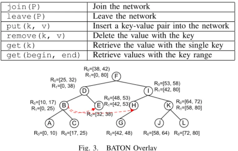
TABLE I BATON INTERFACE
join(P) Join the network
leave(P) Leave the network
put(k, v) Insert a key-value pair into the network
remove(k, v) Delete the value with the key
get(k) Retrieve the value with the single key
get(begin, end) Retrieve values with the key range
F D I B E H K A C J L R0=[0, 10) R0=[10, 17) R1=[0, 25) R0=[17, 25) G R0=[25, 32) R1=[0, 38) R0=[32, 38) R0=[38, 42) R1=[0, 80] R0=[42, 48) R0=[48, 53) R1=[42, 53) R0=[53, 58) R1=[42, 80] R0=[58, 64) R0=[72, 80] R0=[64, 72) R1=[58, 80]
Fig. 3. BATON Overlay
mappings. While the process of extracting and transforming data is straightforward, the main challenge is in maintaining the consistency between raw data stored in the production systems and extracted data stored in the normal peer instance (and subsequently data indices created from these extracted data) when the raw data are updated inside the production systems.
We solve the consistency problem by the following ap-proach. When the data loader first extracts data from the production system, besides storing the results in the normal peer instance, the data loader also creates a snapshot of
the newly inserted data 3. After that, at interval times, the
data loader re-extracts data from the production system to create a new snapshot. This snapshot is then compared to the previously stored snapshot to detect data changes. Finally, the changes are used to update the MySQL database hosted in the normal peer.
Given two consecutive data snapshots, we employ a similar algorithm as the one proposed in [4]. In our algorithm, the system first fingerprints every tuple of the tables in the two snapshots to a unique integer. We use 32Bits Rabin fingerprinting method [14]. Then, each table is sorted by the fingerprint values. Finally, the algorithm executes the sort merge algorithm on the tables in both snapshots. The resultant table after sorting reveals changes in the data.
C. Data Indexer
In the BestPeer++, the data are stored in the local MySQL database hosted by each normal peer. Thus, to process a query, we need to locate which normal peers host the tables involved in the query. For example, to process a simple query like
select R.a from R where R.b=x, we need to know
which peers store tuples belonging to the global tableR. We adopt the peer-to-peer technology to solve the data locating problem and only send queries to normal peers which
host related data. In particular, we employ BATON [9], a
balanced binary tree overlay protocol to organize all normal peers. Figure 3 shows the structure of BATON. Given a value 3The snapshot is also stored in the normal peer instance but in a separate database.
domain [L, U], each node in BATON is responsible for two
ranges. The first range, R0, is the sub-domain maintained by
the node. The second range,R1, is the domain of the subtree
rooted at the node. For example,R0andR1are set to[25,32)
and[0,38)for nodeD, respectively. For a keyk, there is one
unique peer presponsible for k and kis contained by p.R0.
For a range[l, u], there is also one unique peerp¯for it and 1) [l, u] is a sub-range of p.R¯ 1; and 2) if [l, u] is contained by
b
p.R1,pbmust be p¯’s ancestor node.
If we traverse the tree via in-order, we can access the values in consecutive domains. In BATON, each node maintains
log2N routing neighbors in the same level, which are used to
facilitate the search process in this index structure. For details about BATON, readers are referred to [7], [9].
In BestPeer++, the interface of BATON is abstracted as Table I. We provide three ways to locate data required for query evaluation: table index, column index, and range index. Each of them is designed for a separate purpose.
Table Index.Given a table name, a table index is designed
for searching the normal peers hosting the related table. A
table index is of the form IT(key, value) where the key is
the table name andvalueis a list of normal peers which store
data of the table.
Column Index. Column index is a supplementary index
to table index. This index type is designed to support queries
over columns. A column indexIC(key, value)includes a key,
which is the column name in the global shared schema, and a value, which consists of the identifier of the owner normal peer and a list of tables containing the column in the peer.
Range Index. Range indices are built on specific columns
of the global shared tables. One range index is built for one
column. A range index is of the form ID(key, value) where
keyis the table name and the value is a list. Each item in the
list consists of the column name denoting which column the range index is built on, a min-max value which encodes the minimum and maximum value in the column being indexed, and the normal peer which stores the table.
Table II summarizes the index formats in BestPeer++. In query processing, the priorities of indices are (Range
Index>Column Index>Table Index). We will use the more
accurate index whenever possible. ConsiderQ1of the TPC-H
benchmark:
SELECT l orderkey, l receiptdate FROM LineItem WHERE l shipdate > Date(1998-11-05) AND
l commitedate > Date(1998-09-29)
If the range index has been built for l shipdate, the
query processor can know which peers have the tuples with l shipdate > Date(1998-11-05). Otherwise, if col-umn index is available, the query processor only knows which
peers have the LineItem table and their l shipdate
columns have valid values.4In the worst case, when only table
index is available, the query processor needs to communicate with every peer that has part of the lineitem table.
4In multi-tenant scenario, even the companies share the same schema, they may have different set of columns.
TABLE II INDEXFORMATSUMMARIES
Type Key Indexed Value
Table Index Table Name A normal peer list
Column Index Column Name A list of peer-table pairs
Range Index Table Name A list of column-range pairs
Since machine failures in cloud environment are not un-common, BestPeer++ employs replication of index data in the BATON structure to ensure the correct retrieval of index data in the presence of failures. Specifically, we use the two-tier partial replication strategy to provide both data availability and load balancing, as proposed in our recent study [18]. The complete method for system recovery from various types of node failures is also studied in this work.
D. Distributed Access Control
The access to multi-businesses data shared in a corporate network needs to be controlled properly. The challenge is for BestPeer++ to provide a flexible and easy-to-use access control scheme for the whole system; at the same time, it should enable each business to decide the users that can access its shared data in the inherent distributed environment of corporate networks. BestPeer++ develops a distributed role-based access control scheme. The basic idea is to use roles as templates to capture common data access privileges and allow businesses to override these privileges to meet their specific needs.
Definition 1: Access Role
The access role is defined asRole={(ci, pj, δ)|ci∈Sc∧pj ∈
Sp∧δ∈Sv}, whereSc is the set of columns,Spis the set of privileges andSv is the range conditions.
For example, suppose we have created a role
Rolesales={(lineitem.extendedprice, read∧write, [0, 100]), (lineitem.shipdate, read, null) } and a user is assigned the role Rolesales. He can only access two columns. For the
shipdate column, he can access all values, but cannot update them. For the extendedprice column, the user can read and modify the values in the range of[0,100].
When setting up a new corporate network, the service provider defines a standard set of roles. The local administrator at each normal peer can assign the new user with an existing role if the access privilege of that role is applicable to the new user. If none of the existing roles satisfies the new user, the
local administrator can create new roles by three operators:`,
−and+.
• Rolei ` Rolej: Rolej inherits all privileges defined by
Rolei.
• Rolej =Rolei−(ci, pj, δ):Rolej gets all privileges of
Rolei with the exception of(ci, pj, δ).
• Rolej =Rolei+ (ci, pj, δ):Rolej gets all privileges of
Rolei and a new access rule(ci, pj, δ).
The roles are maintained locally and used in the query processing to rewrite the queries. Specifically, given a query
retrieval request to the involved peers. The peer, upon
receiv-ing the request, will transform it based on u’s access role.
The data that cannot be accessed by u will not be returned.
For example, if a user assigned to Rolesale tries to retrieve
all tuples from lineitem, the peer will only return values
from two columns: extendedpriceand shipdate. For
extendedprice, only values in[0,100]are shown, the rest are marked as “NULL”.
Note that BestPeer++ does not collect the information of existing users in the collaborating ERP databases, since it will lead to potential security issues. Instead, the user management module of BestPeer++ provides interfaces for the local administrator at each participating organization to create new accounts for users who desire to access BestPeer++ service. The information of the users created at one peer is forwarded to the bootstrap peer and then broadcasted to other normal peers also. In this manner, each normal peer will eventually have enough user information of the whole network, and therefore the local administrator at this peer can easily define the role-based access control for any user.
V. PAY-AS-YOU-GOQUERYPROCESSING
BestPeer++ provides two services for the participants: the storage service and search service, both of which are charged in a as-you-go model. This section presents the pay-as-you-go query processing module which offers an optimal performance within the user’s budget. We begin with the presentation of histogram generation, a building block for estimating intermediate result size. Then, we present the query processing strategy.
Before discussing the details of query processing, we first define the semantics of query processing in the BestPeer++. After data are exported from the local business system into a BestPeer++ instance, we apply the schema mapping rules to transform them into the predefined formats. In this way, given
a tableT in the global schema, each peer essentially maintains
a horizontal partition of it. The semantics of queries is defined as
Definition 2: Query Semantic
For a query Q submitted at time t, let T denote the tables involved inQ. The result ofQis computed onS
∀Ti∈T St(Ti), where St(Ti)is the snapshot of tableTi at timet.
When a peer receives a query, it compares the timestamp (t0) of its database with the query’s timestamp (t). If t0 ≤t, the peer processes the query and returns the result. Otherwise, it rejects the query and notifies the query processor, which will terminate the query and resubmit it.
A. The Histogram
In BestPeer++, histograms are used to maintain the statistics of column values for query optimization. Since attributes in a relation are correlated, single-dimensional histograms are not sufficient for maintaining the statistics. Instead, multi-dimensional histograms are employed. BestPeer++ adopts MHIST [13] to build multi-dimensional histograms adaptively. Each normal peer invokes MHIST to iteratively split the
attribute which is most valuable for building histograms until enough histogram buckets are generated. Then, the buckets (multi-dimensional hypercube) are mapped into one dimen-sional ranges using iDistance [8] and we index the buckets in BATON based on their ranges.
Once the histograms have been established, we can estimate the size of a relation and the result size of joining two relations as follows.
Estimation of a Relation Size.Given a relationR and its
corresponding histogram H(R),ES(R) =P
iH(R)i, where
H(R)i denotes the value of theithbucket in H(R).
Estimation of Pairwise Joining Result Size. Given two
relations Rx, Ry, their corresponding histograms H(Rx),
H(Ry) and a query q = σp(Rx ./Rx.a=Ry.b Ry), where
p=Rx.a1∧· · ·∧Rx.an−1∧Ry.b1∧· · ·∧Ry.bn−1, to estimate
the joining result size of a query, we first estimate the number of data in each histogram belonging to the queried region(QR)
defined by the predicatepas follows.
EC(H(Rx)) = X i H(Rx)i× Areao(H(Rx)i, QR) Area(H(Rx)i) EC(H(Ry)) = X i H(Ry)i× Areao(H(Ry)i, QR) Area(H(Ry)i)
Where Area(H(Rx)i) and Areao(H(Rx)i, QR) denote the
region covered by theithbuckets ofH(Rx)and the
overlap-ping region between this region andQR. A similar explanation
is applied forArea(H(Ry)i)andAreao(H(Ry)i, QR).
Based on EC(H(Rx)) and EC(H(Ry)), the estimated
result size of qis calculated as follows.
ES(q) =EC(H(Rx))Q×EC(H(Ry))
iWi
whereWi is the width of the queried region at dimensioni.
B. Basic Processing Approach
BestPeer++ employs two query processing approaches: ba-sic processing and extended processing. The baba-sic query pro-cessing strategy is similar to the one adopted in the distributed databases domain. Overall, the query submitted to a normal
peer P is evaluated in two steps: fetching and processing.
In the fetching step, the query is decomposed into a set of subqueries which are then sent to the remote normal peers that host the data involved in the query (the list of these normal peers is determined by searching the indices stored in BATON, cf. Section IV-C). The subquery is then processed by each remote normal peer and the intermediate results are shuffled
to the query submitting peer P.
In the processing step, the normal peer P first collects all
the required data from the other participating normal peers.
To reduce I/O, the peer P creates a set of MemTables to
hold the data retrieved from other peers and bulk inserts these
data into the local MySQL when theMemTableis full. After
receiving all the necessary data, the peer P finally evaluates
the submitted query.
The system also adopts two additional optimizations to speed up the query processing. First, each normal peer caches
sufficient table index, column index, and range index entries in memory to speed up the search for data owner peers, instead of traversing the BATON structure. Second, for equi-join queries, the system employs bloom join algorithm to reduce the volume of data transmitted through the network.
During the query processing, BestPeer++ charges the user for data retrieval, network bandwidth usages and query
pro-cessing. SupposeN bytes of data are processed and the query
consumes tseconds, the cost is represented as:
Cbasic= (α+β)N+γt (1)
whereαandβ denote the cost ratio of local disk and network
usages respectively and γ is the cost ratio for using a
pro-cessing node for a second. Suppose one propro-cessing node can
handle θbytes data per second, the above equation becomes
Cbasic= (α+β)N+γ
N
θ (2)
One problem of the basic approach is the inefficiency of
query processing. The performance is bounded by Nθ, as only
one node is used. We have also developed a more efficient query processing approach that uses more processing nodes. However, the approach will cost more.
C. A Parallel Processing Approach
Aggregation queries and join queries can benefit from
parallel processing 5. By using more processing nodes, we
can achieve a much better query performance. Figure 4 shows an example of the parallel approach. Instead of sending all data to one processing node, we organize multiple processing nodes as a graph and shuffle the data and intermediate results between the graph nodes.
... ...
Basic Approach Extended Approach
Fig. 4. Two query processing approaches.
Definition 3: Processing Graph
Given a query Q, the processing Graph G = (V, E) is generated as follows:
1) For each node vi ∈ V, we assign a level ID to vi, denoted asf(vi).
2) Root nodev0represents the peer that accepts the query, which is responsible for collecting the results for the user.f(v0) = 0.
3) Suppose Q involves x joins and y “Group By” at-tributes, the maximal level of the graph L satisfies
L≤x+f(y)(f(y) = 1, ify≥1. Otherwisef(y) = 0). In this way, we generate a level of nodes for each join operator and the “Group By” operator.
5For simple selection queries, we retrieve data from the remote peers’ databases in parallel.
4) Except for the root node, all other nodes only process one join operator or the “Group By” operator.
5) Nodes of level L accept input data from the Best-Peer++’s storage system (e.g. local databases). After completing its processing, nodevi sends its data to the nodes in levelf(vi)−1.
6) All of operators that are not evaluated in the non-root node are processed by the root.
The processing graph, in fact, defines a query plan, where its non-root nodes are used for improving the query performance via parallelism. Levelirefers to an operator opi. All nodes in
the level are employed to evaluate opi against the input from
leveli+ 1. Letg(i)denote the selectivity ofopi, which can be
estimated via the histograms, the shuffling cost between level
iandi+ 1is estimated as
C(i)s=βΠjL=ig(j)N (3)
Similarly, let D denote the average network bandwidth, the
shuffling time is
T(i)s=
ΠLj=ig(j)N
D (4)
Let mi denotes the number of nodes in level i. The total
number of used nodes is M = PL
i=0mi. Using the same
notion as Equation 2, the processing time is estimated as: Textend= N θM +L L X i=1 T(i)s (5)
And the total cost is estimated as: Cextend= (α+β)N+
L
X
i=1
C(i)s+γM Textend (6)
In our estimation, to simplify the search space, we setmi =
mi+1 for i > 0. Namely, except for level 0, all other levels
have the same number of nodes. In Equation 6, increasing the number of processing nodes leads to a better query per-formance, but also incurs more processing cost. BestPeer++’s query engine adopts an adaptive strategy to follow the pay-as-you-go model.
Definition 4: Pay-As-You-Go Querying Processing
LetT denote the QoS set by the user. The query latency must be less than T seconds with high probability. BestPeer++ generates a plan to minimizeCextend, while guaranteeing that
Textend< T.
BestPeer++’s query engine iterates possible query plans and selects the optimal one. The iteration algorithm is similar to the one used in conventional DBMS and thus is not repeated in the paper. The intuition of the query engine is to exploit the parallelism to meet the QoS and reduce the cost as much as possible.
VI. BENCHMARKING
This section evaluates the performance and throughput of BestPeer++ on Amazon cloud platform. For the performance
benchmark, we compare the query latency of BestPeer++ with HadoopDB using five queries selected from typical corporate network applications workloads. For the throughput bench-mark, we create a simple supply-chain network consisting of suppliers and retailers and study the query throughput of the system.
A. Performance Benchmarking
This benchmark compares the performance of BestPeer++ with HadoopDB. We choose HadoopDB as our benchmark target since it is an alternative promising solution for our problem and adopts an architecture similar to ours. Comparing the two systems (i.e., HadoopDB and BestPeer++) reveals the performance gap between a general data warehousing system and a data sharing system specially designed for corporate network applications.
1) Benchmark Environment: We run our experiments
on Amazon m1.small DB instances launched in the
ap-southeast-1 region. Each DB small instance has
1.7GB memory, 1 EC2 Compute Unit (1 CPU virtual core). We attach each instance with 50GB storage space. We observe that the I/O performance of Amazon cloud is not stable. The hdparm reports that the buffered read performance of each instance ranges from 30MB/sec to 120MB/sec. To produce a consistent benchmark result, we run our experiments at the weekend when most of the instances are idle. Overall, the buffered read performance of each small instance is about 90MB/sec during our benchmark. The end-to-end network
bandwidth between DB small instances, measured byiperf,
is approximately 100MB/sec. We execute each benchmark query three times and report the average execution time. The benchmark is performed on cluster sizes of 10, 20, 50 nodes. For the BestPeer++ system, these nodes are normal peers. We launch an additional dedicated node as the bootstrap peer. For HadoopDB system, each launched cluster node acts as a worker node which hosts a Hadoop task tracker node and a PostgreSQL database server instance. We also use a dedicated node as the Hadoop job tracker node and HDFS name node.
2) BestPeer++ Settings: The configuration of a BestPeer++ normal peer consists of two parts: the underlying MySQL database server and the BestPeer++ software. For MySQL database, we use the default MyISAM storage engine which is optimized for read-only queries since no transactional process-ing overhead is introduced. We set up a large index memory buffer (500MB) and the maximum number of tables to be concurrently opened (50 tables). For BestPeer++ software,
we set the maximum memory consumed by the MemTable
to be 100MB. We also configure each normal peer to use 20 concurrent threads for fetching data from remote peers. Finally, we configure each normal peer to use the basic query processing strategy.
3) HadoopDB Settings: We carefully follow the instruc-tions presented in the original HadoopDB paper to configure HadoopDB. The setting consists of the setup of a Hadoop cluster and the PostgreSQL database server hosted at each worker node. We use Hadoop version 0.19.2 running on Java
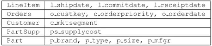
TABLE III
SECONDARYINDICES FORTPC-H TABLES
LineItem l shipdate, l commitdate, l receiptdate
Orders o custkey, o orderpriority, o orderdate
Customer c mktsegment
PartSupp ps supplycost
Part p brand, p type, p size, p mfgr
1.6.0 20. The block size of HDFS is set to be 256MB. The replication factor is set to 3. For each task tracker node, we run one map task and one reduce task. The maximum Java heap size consumed by the map task or the reduce task is 1024MB. The buffer size of read/write operations is set to 128KB. We also set the sort buffer of the map task to 512MB with 200 concurrent streams for merging. For reduce task, we set the number of threads used for parallel file copying in the shuffle phase to be 50. We also enable the buffer reuse between the shuffling phase and the merging phase. As a final optimization, we enable JVM reuse.
For the PostgreSQL instance, we run PostgreSQL version 8.2.5 on each worker node. The shared buffers used by PostgreSQL is set to 512MB. The working memory size is 1GB. We only present the results for SMS-coded HadoopDB, i.e., the query plan is generated by HadoopDB’s SMS planner.
4) Datasets: Our benchmark consists of five queries, de-noted as Q1, Q2, Q3, Q4, and Q5 which are performed on the TPC-H datasets. We design the benchmark queries by ourselves since the TPC-H queries are complex and time-consuming queries and thus are not suitable for benchmarking corporate network applications.
The TPC-H benchmark dataset consists of eight tables. We use the original TPC-H schema as the shared global schema. HadoopDB does not support schema mapping and access control. To benchmark the two systems in the same environ-ment, we perform additional configurations on BestPeer++ as follows. First, we set the local schema of each normal peer to be identical to the global schema. Therefore, the schema mapping is trivial and can be bypassed. We, thus, let the data loader directly load the raw data into the global table without any transformations. Second, we create a unique role
R at bootstrap peer. The unique role is granted full access to
all eight tables. A benchmark user is created at one normal peer for query submitting. All normal peers are configured to
assign the role R to the benchmark user. In summary, in the
performance benchmark, each normal peer contributes data to all eight tables. As a result, to evaluate a query, the query submitting peer will retrieve data from every normal peer.
Finally, we generate the datasets using TPC-H dbgen tool
and produce 1GB data per node. Totally, we generate datasets of 10GB, 20GB, and 50GB for cluster sizes of 10, 20, 50 nodes.
5) Data Loading: The data loading process of BestPeer++ is performed by all normal peers in parallel and consists of two steps. In the first step, each normal peer invokes the data loader to load raw TPC-H data into the local MySQL databases. In addition to copying raw data, we also build indices to speedup
query processing. First, we build a primary index for each TPC-H table on the primary key of that table. Second, we build additional secondary indices on selected columns of TPC-H tables. Table III summarizes the secondary indices that we built. After the data is loaded into the local MySQL database, each normal peer invokes the data indexer to publish index entries to the BestPeer++ network. For each table, the data indexer publishes a table index entry and a column index entry for each column. Since the values in TPC-H datasets follow uniform distribution, each normal peer holds approximately the same data range for each column of the table, therefore, we do not configure normal peer to publish range index.
For HadoopDB, the data loading is straightforward. For each worker node, we just load raw data into the local PostgreSQL database instance by SQL COPY command and build corresponding primary and secondary indices for each table. We do not employ the Global Hasher and Local Hasher to further co-partition tables. HadoopDB co-partitions tables
among worker nodes in order to speed up join processing 6.
However, in a corporate network, the data is fully controlled by each business. The business does not allow moving data to normal peers managed by other businesses. Therefore, we disabled this co-partition function for HadoopDB.
6) The Q1 Query Results: The first benchmark query Q1
evaluates a simple selection predicate on the l shipdate
and l commitdate attributes from the LineItem table. The predicates yields approximately 3,000 tuples per normal peer.
SELECT l orderkey, l receiptdate FROM LineItem WHERE l shipdate > Date(1998-11-05) AND
l commitedate > Date(1998-09-29)
The BestPeer++ system evaluates the query by fetching and processing strategy described in Section V. The query executor
first searches for those peers that hold the LineItemtable.
In our settings, the search will return all normal peers since each normal peer hosts all eight TPC-H tables. Then, the query executor generates a subquery for each normal peer by pushing the selection and projection clause into that peer. The final results are produced by merging partial results returned from data owner peers.
HadoopDB’s SMS planner generates a single MapReduce job to evaluate the query. The MapReduce job only consists of a map function which takes the SQL query, generated by SMS planner, as input, executes the query on local PostgreSQL instance and writes the results into a HDFS file. Similar to BestPeer++, HadoopDB’s SMS planner also pushes projection and selection clause to remote worker nodes.
The performance of each system is presented in Figure 5. Both systems (HadoopDB and BestPeer++) perform this query within a short time. This is because both systems
benefit from the secondary indices built on l shipdate
and l commitdatecolumns. However, the performance of BestPeer++ is significantly better than HadoopDB. The perfor-mance gap between HadoopDB and BestPeer++ is attributed to 6If two tables are co-partitioned on the join column, the join over the two tables can be performed locally without shuffling.
the startup costs of MapReduce job introduced by the Hadoop layer, including the cost of scheduling map tasks on available task tracker nodes and the cost of launching a fresh new Java process on each task tracker node to perform the map task. We note that independent of the cluster size, Hadoop requires approximately 10∼15 seconds to launch all map tasks. This startup cost, therefore, dominates the query processing. BestPeer++, on the other hand, has no such startup cost since it does not require a job tracker node to schedule tasks among normal peers. Moreover, to execute a subquery, the remote normal peer does not launch a separate Java process. Instead, the remote normal peer just forwards that subquery to the local MySQL instance for execution.
7) The Q2 Query Results: The second benchmark query Q2 involves computing the total prices over the qualified tuples
stored in LineItem table. This simple aggregation query
represents another kind of typical workload in a corporate network.
SELECT l returnflag, l linestatus SUM(l extendedprice)
FROM LineItem
WHERE l shipdate > Date(1998-09-01) AND l discount < 0.06 AND
l discount > 0.01 GROUP BY
l returnflag, l linestatus
The query executor of BestPeer++ first searches for peers
that host theLineItemtable. Then, it sends the entire SQL
query to each data owner peer for execution. The partial aggregation results are then sent back to the query submitting peer where the final aggregation is performed.
The query plan generated by the SMS planner of HadoopDB is identical to the query plan employed by BestPeer++’s query executor described above. The SMS compiles this query into one MapReduce and pushes the SQL query to the map tasks. Each map task, then, performs the query over its local PostgreSQL instance and shuffles the results to the reducer side for final aggregation.
The performance of each benchmarked system is presented in Figure 6. BestPeer++ still outperforms HadoopDB by a factor of ten. The performance gap between HadoopDB and BestPeer++ comes from two factors. First, the startup costs introduced by Hadoop layer still dominates the execution time of HadoopDB. Second, Hadoop (and generally MapReduce) employs a pull based method to transfer intermediate data between map tasks and reduce tasks. The reduce task must pe-riodically queries the job tracker for the map completion events and start to pull data after it has retrieved these completion events. We observe that, in Hadoop, there is a noticeable delay between the time point of map completion and the time point of those completion events being retrieved by the reduce task. Such delay slows down the query processing. The BestPeer++ system, on the other hand, has no such delay. When a remote normal peer completes its subquery, it directly sends the results back to the query submitting peer for final processing. That is, BestPeer++ adopts a push based method to transfer intermediate data between remote normal peers and the query
0 5 10 15 20 25 30 50 20 10 Time (sec)
Number of Normal Peers HadoopDB
BestPeer++
Fig. 5. Results for Q1
0 5 10 15 20 25 30 35 40 50 20 10 Time (sec)
Number of Normal Peers HadoopDB
BestPeer++
Fig. 6. Results for Q2
0 10 20 30 40 50 60 70 50 20 10 Time (sec)
Number of Normal Peers HadoopDB
BestPeer++
Fig. 7. Results for Q3
0 10 20 30 40 50 60 50 20 10 Time (sec)
Number of Normal Peers HadoopDB
BestPeer++
Fig. 8. Results for Q4
0 50 100 150 200 250 300 50 20 10 Time (sec)
Number of Normal Peers HadoopDB
BestPeer++
Fig. 9. Results for Q5
6000 8000 10000 12000 14000 16000 18000 20000 5 10 15 20 25 Number of Queries Number of Suppliers Throughput
Fig. 10. Throughput of Suppliers
500 1000 1500 2000 2500 3000 5 10 15 20 25 Number of Queries Number of Retailers Throughput
Fig. 11. Throughput of Retailers
submitting peer. We observe that, for short queries, the push approach is better than pull approach since the push approach significantly reduces the latency between the data consumer (query submitting peer) and the data producer (remote normal peer).
8) The Q3 Query Results: The third benchmark query Q3 involves retrieving qualified tuples from joining two tables,
i.e., LineItemandOrders.
SELECT l orderkey, l shipdate FROM LineItem, Orders
WHERE l orderkey = o orderkey AND
l receiptdate < Date(1994-02-07) AND l receiptdate > Date(1994-01-01) AND o orderdate < Date(1994-01-31) AND o orderdate > Date(1994-01-01)
To evaluate this query, BestPeer++ first identifies the peers
that host LineItem andOrders tables. Then, the normal
peer retrieves qualified tuples from those peers and performs the join.
The query plan produced by SMS planner of HadoopDB is similar to the one adopted by BestPeer++. The map tasks
retrieve qualified tuples of LineItem and Orders tables
and sort those intermediate results based onl orderkey(for
LineItem tuples) and o orderkey (for Orders tuples). The sorted tuples are joined at reducer side using a merge-join algorithm. By default, the SMS planner only launches one reducer to process this query. We found that the default setting yields poor performance. Therefore, we manually set the number of the reducers to be equal to the number of worker nodes and only report results with this manual setting.
Figure 7 presents the performance of both systems. From Figure 7, we can see that the performance gap between BestPeer++ and HadoopDB becomes smaller. This is because this query requires to process more tuples than previous queries. Therefore, the Hadoop startup costs is amortized by the increased workload. We also see that as the number of nodes grows, the scalability of HadoopDB is slightly better than BestPeer++. This is because BestPeer++ performs the final join processing at the query submitting peer. Therefore, the data which are required to process at the query submitting peer grows linearly with the number of normal peers, resulting
in performance degradation. HadoopDB, however, can dis-tribute the final join processing to all worker nodes and thus insensitive to data volume needed to be processed. We should note that, in real deployment, we can boost the performance of BestPeer++ by scaling-up the normal peer instance.
9) The Q4 Query Results: The fourth benchmark query Q4 is as follows.
SELECT p brand, p size, SUM(ps avialqty), SUM(ps supplycost)
FROM PartSupp, Part
WHERE p partkey = ps partkey AND p size < 10 AND ps supplycost < 50
AND p mfgr = ’Manufacturer#3’ GROUP BY p brand, p size
The BestPeer++ system evaluates this query by first fetching qualified tuples from remote peers to query submitting peer
and storing those tuples in MemTables. The BestPeer++,
then, joins tuples stored in theMemTables and produces the
final aggregation results.
The SMS planner of HadoopDB compiles the query into two
MapReduce jobs. The first job joins PartSupp and Part
tables. The SMS planner pushes selection conditions to the map tasks in order to efficiently retrieve qualified tuples by using indices. The join results are then written to HDFS. The second MapReduce job is launched to process the joined tuples and produce the final aggregation results.
Figure 8 presents the performance of both system. We can see that BestPeer++ still outperforms HadoopDB. But the performance gap between the two systems are much smaller. Also, HadoopDB achieves better scalability than BestPeer++. This is because HadoopDB can benefit from parallelism by distributing the join and aggregation processing among worker nodes. However, to achieve that, we must manually set the number of reducers to be equal to the number of worker nodes. BestPeer++, on the other hand, only performs the join and the final aggregation at the query submitting peer. As more nodes are involved, more data need to be processed at the query submitting peer, resulting in that peer to be over-loaded. Again, the performance problem of BestPeer++ can be mitigated by upgrading the normal peer to a larger instance.
10) The Q5 Query Results: The final benchmark query Q5 involves a muti-tables join and is defined as follows.
SELECT c custkey, c name,
SUM(l extendedprice * (1 - l discount)) as R FROM Customer, Orders, LineItem, Nation WHERE c custkey = o custkey
AND l orderkey = o orderkey AND c nationkey = n nationkey AND l returnflag = ’R’
AND o orderdate >= date(1993-10-01) AND o orderdate < date(1993-12-01) GROUP BY c custkey, c name
BestPeer++ evaluates this query by first fetching all qual-ified tuples to the query submitting peer and then do the final join and aggregation processing. HadoopDB compiles this query into four MapReduce jobs with the first three jobs performing the joins and the final job performing the final aggregation.
Figure 9 presents the results of this benchmark. Overall, HadoopDB performs better than BestPeer++ in evaluating this query. The fetching phase of BestPeer++ dominates the query processing since it needs to fetch all qualified tuples to the query submitting peer. HadoopDB, however, can utilize multiple reducers for transferring the data in parallel.
B. Throughput Benchmarking
This Section studies the query throughput of BestPeer++. HadoopDB is not designed for high query throughput, there-fore, we intentionally omit the results of HadoopDB and only present the results of BestPeer++.
1) Benchmark Settings: We establish a simple supply-chain network to benchmark the query throughput of the BestPeer++ system. The supply-chain network consists of a group of
suppliersand a group ofretailerswhich query data from each other. Each normal peer either acts as a supplier or a retailer. We set the number of suppliers to be equal to the number of retailers. Thus, in the cluster with 10, 20, and 50 normal peers, there are 5, 10, and 25 suppliers and retailers respectively.
We still use the TPC-H schema as the global shared schema, but partition the schema into two sub-schema, one for suppliers and the other for retailers. The supplier schema
consists of the following tables:Supplier,PartSupp, and
Part. The retailer schema involves LineItem, Orders,
and Customer tables. The Nation and Region tables
are commonly owned by both supplier peers and retailers peers. We partition the TPC-H datasets into 25 datasets, one dataset for each nation, and configure each normal peer to only host data from a unique nation. The data partition is
performed by first partitioning Customer and Supplier
tables according to their nation keys. Then, joining each SupplierandCustomerdataset with the other four tables
(i.e., Part, PartSupp, Orders, LineItem respectively,
the joined tuples in those tables finally form the corresponding partitioned datasets. To reflect the fact that each table is partitioned based on nations, we modify the original TPC-H schema and add a nation key column in each table. Eventually, we generate a 50GB raw TPC-H dataset and partition the
dataset into 25 supplier datasets and 25 retailer datasets. For a benchmark performed on 10 normal peers, we set 5 normal peers to be suppliers, each of which hosts a unique supplier dataset, and 5 normal peers to be retailers, each of which hosts a unique retailer dataset. The same configuration rule is applied to other cluster sizes in this experiment.
We configure the access control module as follows. We set up two roles: supplier and retailer. The supplier role is granted full access to tables hosted by retailer peers. The retailer role is granted full access to tables hosted by supplier peers. We should not be confused with the supplier role and the supplier peer. The supplier peer is a BestPeer++ normal peer which
hosts tables belonged to a supplier (i.e., Supplier, Part,
PartSupptables). The supplier role is an entity in the access control policy which will be used by a local administrator of a retailer peer to grant users of supplier peers to access tables
(i.e., LineItem, Orders, Customer) hosted at the local
MySQL instance. We also create a throughput test user at each normal peer (either supplier peer or retailer peer) for query submission. Each retailer peer is tasked to assign the supplier role to users from supplier peers. We also let each supplier peer assign the retailer role to users of retailer peers. In this setting, users in retailer peers can access data stored in supplier peers but cannot access data stored in other retailers.
2) Data Loading: The data loading process is similar to the loading process described in Section VI-A.5. The only difference is that in addition to publishing the table indices and column indices, we also build a range index on the nation key column of each table in order to avoid accessing suppliers or retailers which do not host data of interest.
3) Results for Throughput Benchmark: The throughput benchmark queries of suppliers and retailers are as follows:
SELECT s name, s address
FROM Supplier, PartSupp, Part
WHERE p type like ’MEDIUM POLISHED%’ AND p size < 10 AND p availqty < 300 AND s suppkey = ps suppkey AND
p partkey = ps partkey
SELECT l orderkey, o orderdate, o shippriority, SUM(l extendedprice)
FROM Customer, Orders, LineItem WHERE c mktsegment = ’BUILDING’ AND
o orderdate < Date(1995-03-15) AND l shipdate > Date(1995-03-15) AND c custkey = o custkey AND
l orderkey = o orderkey
GROUP BY l orderkey, o orderdate, o shippriotiy
The above queries omit the selection clauses on nation key column to save space. In the actual benchmark, we append a
nation key clause (e.g.,s nationkey = 0) for each table
to restrict the data access on a single supplier or retailer. The benchmark is performed in two rounds: supplier round and retailer round. In the supplier round, the throughput test user at each supplier peer sends retailer benchmark queries to retailer peers. In the retailer round, the throughput test user at each retailer peer sends supplier benchmark queries to supplier peers. In each round, the nation key is randomly
chosen among available nations. Each benchmark query only queries data stored in one retailer or supplier’s database. Each round begins with a 20 minutes warming up. The throughput, namely the number of queries being processed, are collected from the next 20 minutes benchmark.
The supplier benchmark query is light weight. On average, each query is completed in 0.5∼0.6 seconds. The retailer benchmark query, however, is heavy weight, consuming 5∼6 seconds in average per query. We, therefore, benchmark the system in different workloads.
Figure 10 and Figure 11 present the results of this bench-mark. For each setting, the results are presented in separate figures for suppliers and retailers, respectively (e.g., in a 50 node cluster, we have 25 supplier peers and 25 retailer peers). We can see that BestPeer++ achieves near linear scalability in both heavy-weight workloads (i.e., retailer queries) and light-weight workloads(i.e., supplier queries). The main reason for this is that BestPeer++ adopts a single peer optimization. In our benchmark, all queries will only touch just one normal peer. In the peer searching phase, if the query executor finds that a single normal peer hosts all required data, the query executor employs the single peer optimization and sends the entire SQL to that normal peer for execution. The results returned by that normal peer are directly sent back to the user. The final processing phase is entirely skipped.
VII. RELATEDWORK
To enhance the usability of conventional P2P networks, database community have proposed a series of PDBMS (Peer-to-Peer Database Manage System) by integrating the state-of-art database techniques into the P2P systems. These PDBMS can be classified as the unstructured systems such as PIAZZA [17], Hyperion [15] and PeerDB [11], and the structured systems such as PIER [6]. The work on unstructured PDBMS focus on the problem of mapping heterogeneous schemas among nodes in the systems. PIAZZA introduces two materialized view approaches, namely Local As View (LAV) and Global As View (GAV). PeerDB employs information retrieval technique to match columns of different tables. The main problem of unstructured PDBMS is that there is no guarantee for the data retrieval performance and result quality. The structured PDBMS can deliver search service with guaranteed performance. The main concern is the possibly high maintenance cost [1]. To address this problem, partial indexing scheme [20] is proposed to reduce the index size. Moreover, adaptive query processing [21] and online aggre-gation [19] techniques have also been introduced to improve query performance.
The techniques of PDBMS are also adopted in cloud systems. In Dynamo [3], Cassandra [10], and ecStore [18], a similar data dissemination and routing strategy is applied to manage the large-scale data.
VIII. CONCLUSION
We have discussed the unique challenges posed by sharing and processing data in an inter-businesses environment and
proposed BestPeer++, a system which delivers elastic data sharing services, by integrating cloud computing, database, and peer-to-peer technologies. The benchmark conducted on Amazon EC2 cloud platform shows that our system can efficiently handle typical workloads in a corporate network and can deliver near linear query throughput as the number of normal peers grows. Therefore, BestPeer++ is a promising solution for efficient data sharing within corporate networks.
ACKNOWLEDGMENT
This work was in part supported by the Singapore Ministry of Education Grant No. R252-000-454-112. We would also like to thank anonymous reviewers for insightful comments.
REFERENCES
[1] K. Aberer, A. Datta, and M. Hauswirth. Route Maintenance Overheads in DHT Overlays. In The 6th Workshop on Distributed Data and Structures, 2004.
[2] A. Abouzeid, K. Bajda-Pawlikowski, D. J. Abadi, A. Rasin, and A. Sil-berschatz. HadoopDB: An Architectural Hybrid of MapReduce and DBMS Technologies for Analytical Workloads.PVLDB, 2(1):922–933, 2009.
[3] G. DeCandia, D. Hastorun, M. Jampani, G. Kakulapati, A. Lakshman, A. Pilchin, S. Sivasubramanian, P. Vosshall, and W. Vogels. Dynamo: Amazon’s Highly Available Key-Value Store. InSOSP, pages 205–220, 2007.
[4] H. Garcia-Molina and W. J. Labio. Efficient Snapshot Differential Algorithms for Data Warehousing. Technical report, Stanford, CA, USA, 1996.
[5] Google Inc. Cloud Computing-What is its Potential Value for Your Company? White Paper, 2010.
[6] R. Huebsch, J. M. Hellerstein, N. Lanham, B. T. Loo, S. Shenker, and I. Stoica. Querying the Internet with PIER. InVLDB, pages 321–332, 2003.
[7] H. V. Jagadish, B. C. Ooi, K.-L. Tan, Q. H. Vu, and R. Zhang. Speeding up Search in Peer-to-Peer Networks with a Multi-Way Tree Structure. InSIGMOD, 2006.
[8] H. V. Jagadish, B. C. Ooi, K.-L. Tan, C. Yu, and R. Zhang. iDistance: An adaptive b+-tree based indexing method for nearest neighbor search. ACM Trans. Database Syst., 30:364–397, June 2005.
[9] H. V. Jagadish, B. C. Ooi, and Q. H. Vu. BATON: A Balanced Tree Structure for Peer-to-Peer Networks. InVLDB, pages 661–672, 2005. [10] A. Lakshman and P. Malik. Cassandra: structured storage system on a
p2p network. InPODC, pages 5–5, 2009.
[11] W. S. Ng, B. C. Ooi, K.-L. Tan, and A. Zhou. PeerDB: A P2P-based System for Distributed Data Sharing. InICDE, pages 633–644, 2003. [12] Oracle Inc. Achieving the Cloud Computing Vision. White Paper, 2010. [13] V. Poosala and Y. E. Ioannidis. Selectivity estimation without the attribute value independence assumption. In VLDB, pages 486–495, 1997.
[14] M. O. Rabin. Fingerprinting by Random Polynomials, 1981. Harvard Aiken Computational Laboratory TR-15-81.
[15] P. Rodr´ıguez-Gianolli, M. Garzetti, L. Jiang, A. Kementsietsidis, I. Kiringa, M. Masud, R. J. Miller, and J. Mylopoulos. Data Sharing in the Hyperion Peer Database System. InVLDB, pages 1291–1294, 2005. [16] Saepio Technologies Inc. The Enterprise Marketing Management
Strat-egy Guide. White Paper, 2010.
[17] I. Tatarinov, Z. G. Ives, J. Madhavan, A. Y. Halevy, D. Suciu, N. N. Dalvi, X. Dong, Y. Kadiyska, G. Miklau, and P. Mork. The piazza peer data management project.SIGMOD Record, 32(3):47–52, 2003. [18] H. T. Vo, C. Chen, and B. C. Ooi. Towards elastic transactional cloud
storage with range query support. PVLDB, 3(1):506–517, 2010. [19] S. Wu, S. Jiang, B. C. Ooi, and K.-L. Tan. Distributed online
aggregation. PVLDB, 2(1):443–454, 2009.
[20] S. Wu, J. Li, B. C. Ooi, and K.-L. Tan. Just-in-time query retrieval over partially indexed data on structured p2p overlays. InSIGMOD, pages 279–290, 2008.
[21] S. Wu, Q. H. Vu, J. Li, and K.-L. Tan. Adaptive multi-join query processing in pdbms. InICDE, pages 1239–1242, 2009.