In: Proceedings of the fifth international conference on adaptive computing in design and manufacture (ACDM 2002)
Full Elite Sets for Multi-objective
Optimisation
Richard M. Everson, Jonathan E. Fieldsend, Sameer Singh Department of Computer Science
University of Exeter, Exeter, EX4 4PT, UK.
{R.M.Everson,J.E.Fieldsend,S.Singh}@exeter.ac.uk
Abstract
Multi-objective evolutionary algorithms frequently use an archive of non-dominated solutions to approximate the Pareto front. We show that the truncation of this archive to a limited number of solutions can lead to oscillating and shrinking estimates of the Pareto front. New data structures to permit efficient query and update of the full archive are proposed, and the superior quality of frontal estimates found using the full archive is illustrated on test problems.
1 Introduction
Genetic algorithms and evolutionary techniques have been successfully used for a number of years for the optimisation of single objectives. However, one often desires the optimisation of more than one objective, for example, product performance and cost of production. In [1], for example, multi-objective optimisation is applied to four performance measures of a gas turbine, and in [2] different loads in trusses are the competing objectives to be minimised. Recently different measures of a neural network’s performance for financial prediction have been optimised [3]. In all these cases a single solution will seldom optimise all objectives, and the goal of optimisation methods is to discover solutions that lie on the curve (for two objectives) or surface (more than two objectives) that describes the optimal trade-off possibilities between objectives. This surface is known as the Pareto front and solutions lying on it are known as non-dominated solutions. A non-dominated solution lying on the Pareto front cannot improve any objective without degrading at least one of the others, and, given the constraints of the model, no solutions exist beyond the Pareto front.
Although evolutionary methods have been used in multi-objective optimisation for many years, there has been recent renewed practical and theoretical interest in multi-objective genetic algorithms (MOEAs) [1, 4, 5, 6]. In a comparative study Zit-zler et al. [7] show that their Strength Pareto Evolutionary Algorithm (SPEA) out-performs other algorithms on a variety of standard test problems.
Laumanns et al. [8] have presented a unified model for multi-objective evolution-ary algorithms (UMMEA), of which SPEA is an example. Algorithms in this class extend the notion of elitism to multi-objective algorithms by maintaining an archive or frontal set,Ft,of non-dominated solutions, in addition to the usual GA population, Bt. As the evolutionary algorithm proceeds this archive set comprises the current es-timate of the Pareto front. It is also actively used in the search process as part of the cross-over process to generate new individuals, rather than being a mere static store of the best solutions found.
For computational reasons the archive is of fixed size in SPEA: if it were allowed to grow without bound the cost of searching it to discover whether new solutions should be added to it becomes prohibitive. However, fixing the size of the archive can lead to defects in the the speed and stability of the SPEA and algorithms like it, manifest in the form of shrinking, oscillating and retreating estimates of the Pareto front. In this paper we describe some of the problems inherent in representing the Pareto front by a limited number of solutions, and we present a novel data structure, the dominated tree, for storing the non-dominated solutions.
2 Background
The notions of non-dominance and Pareto optimality, which we briefly review, are central to most MOEAs. Without loss of generality we assume that the multi-objective problem seeks to minimise D objectives, yi = fi(x), i = 1, . . . , D, where each objective depends onx, aP-dimensional vector of parameters. The multi-objective optimisation problem may be succinctly stated as:
Minimise y=f(x) = (f1(x), . . . , fD(x)) (1) subject to e(x) = (e1(x), . . . , eJ(x))≥0 (2)
wherex = (x1, x2, . . . , xP)andy = (y1, y2, . . . , yD)andej(x), j = 1, . . . , J are
constraints upon the solution.
When there is more than one objective to be minimised it is clear that there may be solutions for which performance on one objective cannot be improved without sacrificing performance on at least one other. Such solutions are said to be Pareto optimal [9] and the set of all Pareto optimal solutions is said to form the Pareto front. The notion of dominance may be used to make Pareto optimality more precise. A decision vectoruis said to strictly dominate anotherv(denotedu≺v) iff
fi(u)≤fi(v) ∀i= 1, . . . , D (3) and fi(u)< fi(v) for some i (4) Less stringently,uweakly dominatesv(denoteduv) iff
fi(u)≤fi(v) ∀i= 1, . . . , D (5) A set ofM decision vectors{wi}is said to be a non-dominated set (an estimate of the Pareto front) if no member of the set is dominated by any other member:
t:= 0 (F0, B0, pe0) =initialise() whileterminate(Ft, Bt, pe t) =false: t:=t+ 1 Ft0 :=update(Ft−1, Bt−1) Ft:=truncate(Ft0) pet :=adapt(Ft, Bt−1, pet−1) Bt:=vary(sample(evaluate(Ft, Bt, pet))) end
Figure 1. The sequential unified multi-objective evolutionary algorithm [8]. Ft denotes the
elite archive,Btthe general population andpet the elitism intensity at generationt.
3 UMMEAs
Laumanns et al. [8] have described a general framework for multi-objective evolu-tionary algorithms incorporating elitism. Fig. 1 summarises the sequential UMMEA framework in terms of various stochastic operators. The general genetic population B0is initialised, together with the elite setF0which is generally initialised to be the
empty set. At each generation, the elite set is augmented to formFt0by incorporating those solutions inBt−1which are not dominated any member ofFt−1∪Bt−1; also any
elements of theFt−1which are dominated by members ofBt−1are deleted fromFt0. For computational reasons, the updated frontal set is then truncated (usually to some fixed size). In the SPEA this truncation is achieved by clustering. In the final stage of the algorithm the fitness of individuals is evaluated and used to control the sampling of individuals from both the frontal set and the search population for crossover and mutation to yield an offspring populationBt. The crossover and mutation operators are abstractly represented by the vary() operator. In SPEA [10] and a recent extension to SPEA [11] fitness ofxis evaluated according to the number of individuals inFt dominatingx.
The ‘elitism intensity’,pe
t,controls the probability that an individual from the elite archive set will be selected for the binary tournament [8]. A straight-forward scheme is to choosepe
t =|Bt|/|Ft|so that equal numbers of individuals are chosen fromBt andFt. In [11] a more sophisticated method for sampling fromFtis described which ensures that all regions of the front are equally well represented in the population entering the binary tournament. This prevents the search from concentrating in regions in which there are already many individuals and thus forces exploration along the entire estimated Pareto front.
3.1 Truncation
The archive of elite solutions forms the best estimate of the Pareto front at any stage. It should therefore ‘advance’ in the sense that no individual inFtshould be dominated by any member of an earlier frontal set, F0, . . . , Ft−1. Informally, we say that an
Figure 2. A retreating archive set produced by clustering. Panels illustrate the elite set at successive generations. Elements ofFtare shown as open circles, those entering are shown as
filled circles, and elements to be clustered are circled.
individualxlies behind the front if a member of the frontal set dominatesx.
The truncation stage of UMMEAs, introduced to control the size ofFtand thus the space required to store it, and, more crucially, the time required to search it, can be deleterious: in particular, the front can fail to advance and instead may retreat or oscillate.
In SPEA, for example,Ftis truncated by clustering members ofFtaccording to their separation in objective space and then replacing clusters with the member closest to the cluster centroid.
The effect of clustering is illustrated in Fig. 2. Fig. 2a illustrates an archive set with a maximum ofM = 6members. In Fig. 2b a new non-dominated member (drawn as a filled circle) has entered the set. Since there are now7elements in the frontal set, one must be removed by clustering; the pair of solutions nearest each other form a cluster of two and one of them (chosen at random) is deleted, resulting in the set shown in Fig. 2c. If at a subsequent generation a new element enters the frontal set (Fig. 2d), the clustering process will reduce the frontal set as shown in Fig. 2e to yield a frontal set (Fig. 2f) containing an element that lies behind (is dominated by) elements of the original frontal set (Fig. 2a). Repeated occurrences of this process can lead to the estimated front retreating or, more commonly, oscillating as the front advances in the search stage but retreats during clustering.
This artifact has two principal consequences. First, search time is wasted ‘redis-covering’ individuals and regions that have been eliminated by clustering. Secondly, numerical simulations show that this oscillation is particularly serious when the es-timated front lies close to the true front; the oscillation can prevent convergence to
the true front, leading to poor estimates and difficulties in assessing convergence. Al-though the artifact has been illustrated here using clustering to limit|Ft|other trunca-tion methods suffer from the same artifacts.
In order to counter this artifact we propose that all non-dominated solutions are retained to form the archive or frontal setFt. Such a frontal set has the desirable property that it cannot retreat or oscillate. The frontal set therefore always moves towards the true Pareto front. In addition to improving the efficiency of the algorithm, this property also permits sensible convergence criteria to be defined.
4 Dominated trees
As the frontal set contains all the currently non-dominated decision vectors found, it may become very large as the search progresses. Since, at each generation, Ft must be queried to discover whether elements of it are dominated by elements of the search population and vice versa, linear-time query, deletion and insertion can become prohibitive. Data structures to facilitate searchingFtin logarithmic time are the dominated and non-dominated trees.1
Sun & Steuer have also described a modification to quadtrees for maintaining non-dominated sets [12], and the PAES [13] and PEAS [14] algorithms are both based upon recursively dividing objective space into hyper-rectangles that could be supported by quadtrees; however, both algorithms truncate the archive set.
Here it is convenient to regard members of the frontal set and individuals from the search population as pointsy in D-dimensional space. Geometrically, finding individuals inFthat dominateyamounts to finding frontal individuals that lie to the ‘south-west’ or ‘left and below’y.
The ‘dominates’ relation imposes a partial order on individuals. However, since the elements ofF are mutually non-dominating, this relation cannot be used directly to construct, for example, a binary tree to enable fast searching.
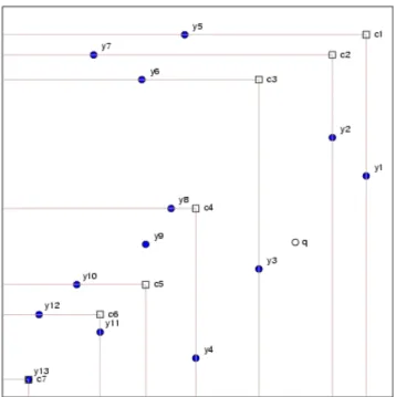
The dominated tree consists of an ordered list of composite points (usually stored as binary tree). Each composite point represents (upto)Delements ofF and compos-ite points are defined so that they are ordered by the weakly-dominates relation,. An example of a dominated tree is shown in Fig. 3.
The essential property of dominated trees is that the composite points are ordered:
cicj iffi > j (7)
Usually, the stronger condition,ci ≺cj iffi > j, will hold. In addition, ifcj ci then the constituent points ofci also dominatecj. Thus, for example, in Fig. 3 the constituent points ofc4,c5c6 andc7 dominatec3. Note, however, that they do not
necessarily dominate the constituent points ofc3,namelyy3andy6.
It should be emphasised that the points forming the tree in Fig. 3 do not form a non-dominated set. This is for expository purposes, because non-dominated sets in two dimensions have the peculiar property that listing the points in order of increasing
1An example implementation of dominated and non-dominated trees is available fromhttp://www.
Figure 3. A dominated tree. 13 pointsymin two dimensions and the composite pointsci
(squares) forming a dominated tree. The open circle,q, marks a query point. Composite nodes listed are: c1 = (y1,y5) c2 = (y2,y7) c3 = (y3,y6) c4 = (y4,y8) c5 = (y9,y10)c6= (y11,y12)c7= (y13,y13).
first coordinate (objective), y1, is equivalent to listing them in order of decreasing
second coordinate,y2. With more than two objectives this is no longer the case and
the points illustrated in Fig. 3 are more akin to the general case.
Construction. Construction of a dominated tree fromM =|F|pointsF ={ym}M1
proceeds as follows. The first composite pointc1is constructed by finding the point
ymwith maximum first coordinate; this value forms the first coordinate of the com-posite point:
c1,1= max
F ym,1 (8)
This pointymis now associated withc1and deleted fromF. Likewise, the second coordinate ofc1 is the maximum second coordinate of the points remaining in F, thusc1,2 = maxFym,2. In this manner each coordinate of c1 is defined in turn.
The process is then repeated to constructc2and subsequent points untilF is empty.
Note that in construction of the final composite point, (that is, the composite point that dominates all other composite points)Fmay be empty before theDcoordinates of the composite point have been defined. As illustrated byc7in Fig. 3, in this case theym (y13in Fig. 3) already comprising the composite point serve to define the coordinates
Since (except possibly for the dominating composite point)Delements ofF are used in the construction of each composite point, the maximum number of composite points isdM/De.
Although we have described the construction of a dominated tree from a static frontal set, dynamic insertion and deletion are straight-forwardly accomplished, to-gether with a rebalancing or ‘cleaning’ operation [11].
Query. Given a test pointq, the properties of dominated trees can be used to dis-cover which points inFdominateq. Although the dominated tree may conveniently be implemented as a binary tree, the query procedure is most easily described in terms of an ordered list ofL=dM/Decomposite points. First, the list is searched to find the indiceshandlof composite pointschandclthat dominate and are dominated by
qrespectively: l= 0ifc1≺q max{i : ci≺q} otherwise (9) and h= L+ 1ifciq min{i : ciq} otherwise (10) Also, denote bycH the ‘least’ composite point that strictly dominatesch:
H = min{i : ci ≺ch} (11) For the query point illustrated in Fig. 3,l = 2,h= 5andH = 6. (Note that it is not necessarily true thatH =h+ 1.) Sincech≺qit is clear that all the constituent points of the composite pointsci that dominatech,H ≤ i ≤ L, also dominateq. (Note that the constituent points ofch(and indeed andci) that only weakly dominate
ch, need not dominate q; in Fig. 3 c5 ≺ q, but y9 ⊀ q.) Also, since q ≺ cl and the constituent points ofclhave at least one coordinate equal to a coordinate of
cl, it may be concluded thatqis not dominated by any of the constituent points of
c1, . . .cl. Each constituent pointciwithl < i < Hmust be checked individually to determine whether it dominatesq; in Fig. 3 the pointsy3,y6,y4,y8,y9,y10must be
individually checked.
Note that when determining whetherqis to be included in F,qcan be imme-diately rejected ifh < L because it is certainly dominated by at least one of the constituents ofcL.
Since the composite points are arranged as a sorted list, determination of l and htakesO(lg(M/D))comparisons each. Hence the total number of comparisons re-quired isO(2 lg(M/D)+K), whereKis the number of points that have to be checked individually. Clearly, certain configurations ofF andqcan result in all elements ofF being checked — in linear time. However, such arrangements are seldom encountered in practice and the logarithmic query time permits the use of very large frontal sets.
If it is determined that qis to be included in F (because it is not dominated by any element ofF), those elements ofFwhich are dominated byqmust be identified and deleted fromF. Queries about which elements ofF are dominated byqcan be answered using the dominated tree, however, it may be inefficient. This is because
althoughq ≺ ci for i ≤ l,qneed not dominate the constituent points of these ci and the constituent points must therefore be checked individually. Thus in Fig. 3,
q ≺c2 ≺c1, buty5andy7are not dominated byq. The non-dominated tree is a data structure which permits this sort of query to be answered efficiently.
Non-dominated are analogous to dominated trees. A non-dominated tree consists of a ordered composite points, ci cj iffi < j, with the additional property that ifci cj, then the constituent points ofcj are also dominated byci. Construction and querying of non-dominated trees is analogous to dominated trees and they are not discussed further here.
5 Numerical example
We briefly illustrate the benefits of retaining all non-dominated solutions by com-paring the performance of SPEA [10] and E-SPEA [11], a modification of SPEA which retains all non-dominated solutions. Although standard benchmark functions for MOEAs exist [7], these are peculiar in that the first objective,y1depends solely
on the single parameterx1. We therefore prefer to use the more severe test functions
which are defined in terms of the following five base functions: B1(x) = P X i=1 |xi− 1 3expi/m 2 |12 B2(x) = P X i=1 [xi−1 2(cos (10π(i/m)) + 1)] 2 B3(x) = P X i=1 xi−sin2(i−1) cos2(i−1) 1 2 B4(x) = P X i=1 |xi−1 4(cos (i−1) cos (2 (i−1)) + 2)| 1 2 B5(x) = P X i=1 [xi− 1 2(sin (1000π(i/m)) + 1)] 2
where m = 30 andxi∈[0,1]. We then define the following two-dimensional test func-tions: F1(x) = (B1(x), B2(x)),F2(x) = (B3(x), B4(x)),F3(x) = (B3(x), B5(x)),
the three-dimensional objective function,F4(x) = (B1(x), B4(x), B5(x))and the
four-dimensional functionF5(x) = (B1(x), B3(x), B4(x), B5(x)).
A detailed discussion of measures for comparing non-dominated sets is given in [11]. Here we compare two non-dominated sets,AandB, byV(A, B)∈[0,1]which measures the fraction of the volume of the minimum hypercube containing both fronts that is strictly dominated by members ofAbut is not dominated by members ofB.
V(A, B)is defined as follows. For any set ofD-dimensional vectorsY, letHY denote the smallest axis-parallel hypercube containingY:
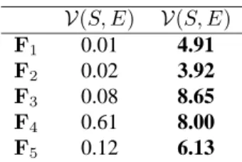
V(S, E) V(S, E) F1 0.01 4.91 F2 0.02 3.92 F3 0.08 8.65 F4 0.61 8.00 F5 0.12 6.13
Table 1. Comparison of SPEA and E-SPEA on five test functions. V(S, E) measures the percentage of objective space dominated by the SPEA front but not dominated by the E-SPEA front, whileV(S, E)measures the fraction dominated by the E-SPEA front but not by the SPEA front. Figures in bold are significant at the 2% level (Wilcoxon signed ranks test).
Now denote byhY (y) :HY 7→[0,1]D the normalising scaling and translation that mapsHY onto the unit hypercube. This transformation serves to remove the effects of scaling the objectives. Finally, let
DY (A) ={z∈[1,0]D : z≺hY (a), a∈A} (13) be the set of points in the unit cube which are dominated by the normalised elements ofA. ThenV(A, B)is defined as
V(A, B) =λ DAS
B(A)\DAS
B(B)
(14) whereλ(A)denotes the Lebesgue measure ofA.
Despite this awkward definition, V(A, B)andV(B, A)are easily calculated by Monte Carlo sampling ofHASBand counting the fraction of samples that are
domi-nated exclusively byAorB.V(A, B)is insensitive to spatial distribution of elements in the setsAandB, as well as rescaling of the objective axes. Note, however, that
V(A, B)6=V(B, A)sinceAmay dominate parts ofBwhileBdominates parts ofA. Also note that ifW is a non-dominating set, andA⊆W andB ⊆W,V(A, B)and
V(B, A)may both be positive.
5.1 Results
Table 1 shows a comparison of the fronts found by an implementation of SPEA [10] and E-SPEA, an extended version of ESPEA which retains all non-dominated solu-tions [11].
The two EAs were each executed 30 times on each test problem, and the resultant non-dominated solutions saved at the end of each run. In the case of E-SPEA these were simply those individuals residing inFat the end of run, whereas an off-line store of the non-dominated solutions discovered by SPEA was kept. For both algorithms the|Bt| = 80. In SPEAFtwas limited to 20 individuals (the same number as used in SPEA studies [7]), all of whom were entered into the binary tournament selection for breeding; in E-SPEA 20 individuals for breeding were selected quasi-randomly, ensuring a spatially uniform distribution across the front (see [11] for details). Both algorithms used single point crossover with a crossover rate of 0.8 and a mutation rate
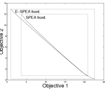
Figure 4. Empirical fronts. The two estimated Pareto fronts generated by SPEA and E-SPEA for test functionF1. The non-dominated individual from 30 separate runs of 2500 generations
are plotted.
of 0.01. In each of the 30 different runs E-SPEA and SPEA were initialised from identical decision vector populations, andx0
i ∼U(0,1).
Denoting the aggregate frontal set after 2500 generations from SPEA and E-SPEA bySandErespectively, table 1 showsV(S, E)andV(E, S). These results indicate that the E-SPEA frontal set lies substantially ‘in front’ of that found by SPEA, al-though the fact thatV(S, E)>0indicates that there are regions were the SPEA front is ‘in front’. Fig. 5.1 shows the two estimated Pareto fronts for test functionF1. It is clear that not only is the E-SPEA front substantially ‘in front’ of the SPEA front, it is also of wider extent: another artifact of truncation is that the front tends to shrink as extremal solutions are discarded by clustering and other forms of truncation.
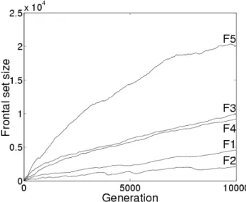
It is worth noting that although the frontal set may become large, its rate of increase is at most linear, because at most|Bt|individuals may be added at any generation. Indeed Fig. 5 shows that the rate is far smaller than this maximum. Nonetheless Fig. 5 indicates that frontal sets of several hundreds are quickly encountered, necessitating efficient structures for manipulating them.
6 Conclusion
We have argued that truncation of the archive of non-dominated solutions in MOEAs is detrimental to their performance. Truncation is detrimental to both the quality of the approximation to the true Pareto front and to the rate of convergence. The theoretical argument is supported by empirical results on realistic test functions. Truncation is usually introduced for computational expediency, to avoid the expense of searching
Figure 5. Size of frontal set. Number of non-dominated individuals located by E-SPEA versus generation.
through a large archive of non-dominated solutions at each generation. To relieve the burden of a linear search we have introduced the dominated and non-dominated tree data structures which permit logarithmic time search.
Retaining all non-dominated solutions confers a desirable property on the frontal set, namely that it can only ‘advance’: solutions in the archive cannot be dominated by any solution from a previous generation. This property, in turn, permits the introduc-tion of robust stopping criteria that have so far been absent from the MOEA literature [11].
References
[1] C.M. Fonseca and P.J. Fleming. Genetic Algorithms for Multiobjective Opti-mization: Formulation, Discussion and Generalization. In Proceedings of the Fifth International Conference on Genetic Algorithms, pages 416–423, San Ma-teo, California, 1993. Morgan Kaufmann. URLciteseer.nj.nec.com/ fonseca93genetic.html.
[2] P. Hajela and C-Y. Lin. Genetic search strategies in multicriterion optimal de-sign. Structural Optimization, 4:99–107, 1992.
[3] J.E. Fieldsend and S. Singh. Pareto Multi-Objective Non-Linear Regression Modelling to Aid CAPM Analogous Forecasting. In Proc. IEEE Intl. Conf. on Computational Intelligence for Financial Engineering, 2002.
for Multiobjective Optimization. In Proceedings of the First IEEE Conference on Evolutionary Computation, IEEE World Congress on Computational Intel-ligence, volume 1, pages 82–87, Piscataway, New Jersey, 1994. IEEE Service Center. URLciteseer.nj.nec.com/horn94niched.html.
[5] J.D. Schaffer. Multiple objective optimization with vector evaluated genetic al-gorithms. In Proc. of the First Int. Conf. on Genetic Algorithms, pages 99–100, 1985.
[6] N. Srinivas and K. Deb. Multiobjective Optimization Using Nondominated Sort-ing in Genetic Algorithms. Evolutionary Computation, 2(3):221–248, 1995. URLciteseer.nj.nec.com/srinivas94multiobjective.html. [7] E. Zitzler, K. Deb, and L. Thiele. Comparison of Multiobjective Evolutionary Algorithms: Empirical Results. Evolutionary Computation, 8(2):173–195, 2000. URLciteseer.nj.nec.com/zitzler99multiobjective.html. [8] M. Laumanns, E. Zitzler, and L. Thiele. A Unified Model for Multi-Objective
Evolutionary Algorithms with Elitism. In Proc. of the 2000 Congress on Evol. Comp., pages 46–53. IEEE, 2000.
[9] D. Van Veldhuizen and G. Lamont. Multiobjective Evolutionary Algorithms: Analyzing the State-of-the-Art. Evolutionary
Com-putation, 8(2):125–147, 2000. URL citeseer.nj.nec.com/
vanveldhuizen00multiobjective.html.
[10] E. Zitzler. Evolutionary Algorithms for Multiobjective Optimization: Methods and Applications. PhD thesis, Swiss Federal Institute of Technology Zurich (ETH), 1999. Diss ETH No. 13398.
[11] J.E. Fieldsend, R.M. Everson, and S. Singh. Extensions to the Strength Pareto Evolutionary Algorithm. IEEE Trans. Evol. Comp., 2001. URLwww.dcs.ex. ac.uk/people/reverson. (submitted).
[12] M. Sun and R.E. Steuer. InterQuad: An interactive quad tree based procedure for solving the discrete multiple criteria problem. European Journal of Operational Research, 89:462–472, 1996.
[13] Joshua D. Knowles and David Corne. Approximating the nondom-inated front using the pareto archived evolution strategy. Evolution-ary Computation, 8(2):149–172, 2000. URL citeseer.nj.nec.com/ knowles00approximating.html.
[14] D. W. Corne, J. D. Knowles, and M. J. Oates. The pareto envelope-based se-lection algorithm for multiobjective optimization. In Hans-Paul Schwefel Marc Schoenauer, Kalyanmoy Deb, Günter Rudolph, Xin Yao, Evelyne Lutton, Juan Julian Merelo, editor, Parallel Problem Solving from Nature - PPSN VI 6th International Conference, Paris, France, 16-20 2000. Springer Verlag. URL citeseer.nj.nec.com/corne00pareto.html.