San Jose State University
SJSU ScholarWorks
Master's Projects Master's Theses and Graduate Research
Spring 2018
Image Spam Classification using Deep Learning
Ajay Pal Singh
San Jose State UniversityFollow this and additional works at:https://scholarworks.sjsu.edu/etd_projects
Part of theComputer Sciences Commons
This Master's Project is brought to you for free and open access by the Master's Theses and Graduate Research at SJSU ScholarWorks. It has been accepted for inclusion in Master's Projects by an authorized administrator of SJSU ScholarWorks. For more information, please contact
Recommended Citation
Singh, Ajay Pal, "Image Spam Classification using Deep Learning" (2018).Master's Projects. 641. DOI: https://doi.org/10.31979/etd.wehw-dq4h
Image Spam Classification using Deep Learning
A Project Presented to
The Faculty of the Department of Computer Science San Jose State University
In Partial Fulfillment
of the Requirements for the Degree Master of Science
by Ajay Pal Singh
c ○2018 Ajay Pal Singh ALL RIGHTS RESERVED
The Designated Project Committee Approves the Project Titled
Image Spam Classification using Deep Learning
by Ajay Pal Singh
APPROVED FOR THE DEPARTMENT OF COMPUTER SCIENCE
SAN JOSE STATE UNIVERSITY
May 2018
Dr. Katerina Potika Department of Computer Science
Dr. Mark Stamp Department of Computer Science
ABSTRACT
Image Spam Classification using Deep Learning by Ajay Pal Singh
Image classification is a fundamental problem of computer vision and pattern recognition. Spam is unwanted bulk content and image spam is unwanted content embedded inside the images. Image spam creates threat to the email based communi-cation systems. Nowadays, a lot of unsolicited content is circulated over the internet. While a lot of machine learning techniques are successful in detecting textual based spam, this is not the case for image spams, which can easily evade these textual-spam detection systems. In this project, we explore and evaluate four deep learning tech-niques that detect image spams. First, we study neural networks and the deep neural networks, which we train on various image features. We explore their robustness on an improved dataset, which was especially build in order to outsmart current image spam detection techniques. Finally, we design two convolution neural network ar-chitectures and provide experimental results for these alongside the existing VGG19 transfer learning model for detecting image spams. Our work offers a new tool for detecting image spams and is compared against recent related tools.
ACKNOWLEDGMENTS
I would like to express my gratitude to my advisor, Prof. Katerina Potika and my committee members Prof. Robert Chun and Prof. Mark Stamp for investing their time in this work and giving their valuable feedback. I would like to thank the staff members of computer science department at San Jose State University for their guidance. I am grateful to my peer students and friends who helped me in providing suggestions and feedback regarding my work. Finally I would like to thank my family members: my parents and my sisters for their constant support and motivation which helped me spiritually and mentally throughout this project and my life in general.
TABLE OF CONTENTS
CHAPTER
1 Introduction . . . 1
2 Problem Statement and Motivation . . . 3
2.1 Problem Statement . . . 3 2.2 Motivation . . . 4 3 Background . . . 5 3.1 Spam Categories . . . 5 3.2 Classification Techniques . . . 6 3.2.1 Neural Networks . . . 6
3.2.2 Deep Neural Networks . . . 7
3.2.3 Convolution Neural Networks . . . 8
3.2.4 Transfer Learning . . . 11 3.3 Other Terminologies . . . 12 4 Related Work . . . 15 5 Framework . . . 18 5.1 Datasets . . . 18 5.1.1 Dredze Dataset . . . 18
5.1.2 Image Spam Hunter (ISH) . . . 18
5.1.3 Improved Dataset . . . 19
5.1.4 Combined dataset . . . 19
5.3 Image Features . . . 20 5.3.1 Metadata Properties . . . 20 5.3.2 Color Properties . . . 21 5.3.3 Texture Properties . . . 22 5.3.4 Shape Properties . . . 22 5.3.5 Noise Properties . . . 24 5.4 Techniques Used . . . 25 5.4.1 Neural Networks . . . 26
5.4.2 Deep Neural Networks . . . 26
5.4.3 Convolution Neural Network . . . 27
5.4.4 Transfer Learning . . . 29
6 Experimental Results . . . 31
6.1 Neural Network . . . 31
6.1.1 Image Spam Hunter Dataset . . . 31
6.1.2 Dredze Dataset . . . 33
6.2 Deep Neural Network . . . 36
6.2.1 Image Spam Hunter . . . 36
6.2.2 Dredze Dataset . . . 37
6.3 Convolution Neural Network & Transfer Learning . . . 39
7 Conclusion & Future Work . . . 42
LIST OF FIGURES
1 A multi-layer perceptron with one hidden layer . . . 7
2 Visualization of 5x5 filter convolving around input volume and pro-ducing activation map . . . 10
3 Maxpooling of 2x2 filter and a stride of 2 . . . 11
4 A simple CNN architecture composed of different layers . . . 11
5 A Confusion Matrix [1] . . . 13
6 SPAM vs HAM RGB’s histogram . . . 21
7 SPAM vs HAM HSV’s histogram . . . 22
8 a) HAM original Image b) HAM Grayscale Image c) HAM HOG d) HAM Canny edges . . . 23
9 a) SPAM original Image b) SPAM Grayscale c) SPAM HOG d) SPAM Canny edges . . . 24
10 Different Image Features . . . 25
11 NN Architecture . . . 26
12 VGG19 architecture . . . 30
13 ROC curve for NN trained on ISH dataset . . . 32
14 Confusion Matrix for ISH trained on NN . . . 32
15 ROC curve for NN when trained on Improved dataset combined with ISH dataset . . . 33
16 ROC & Confusion Matrix for Dredze dataset trained on NN . . . 34
17 ROC curve for Dredze dataset combined with improved dataset on NN . . . 34
19 ROC & Confusion Matrix for ISH dataset trained on DNN . . . . 36
20 ROC curve for ISH dataset combined with improved dataset and trained on DNN . . . 37
21 ROC & Confusion Matrix for Dredze dataset trained on DNN . . 38
22 ROC curve for Dredze dataset combined with improved dataset on DNN . . . 38
23 Summarized Result of DNN trained on different datasets . . . 39
24 Accuracy vs Loss for CNN1 model . . . 40
CHAPTER 1 Introduction
Over the last decade, email and internet is flooded with spam content. A spam can be defined as unwanted content, distributed mostly via emails. Due to the efflu-ence of spam emails over the Internet a lot of techniques have surfaced which classify the spam from the valid content. Reports from Symantec [2] indicated that 90.4% of the emails includes spam content. These spam emails can include phishing links, malwares, advertisements, adult content, etc., which may impose a significant threat to the security of the user’s privacy.
Spam in its initial days was only in the form of texts. With the advent of machine learning, many classifiers were developed to filter such spam based on email content. Lai and Tsai [3] used four different machine learning techniques including K-Nearest Neighbors (KNN), Support Vector Machines (SVM) and Naïve Bayes, which used email messages to filter spam emails. These classifiers were able to classify text based spam with approximately 95% accuracy. Hence, over the years detecting content based spam emails became very easy. Google, Microsoft, Yahoo used techniques which perform very accurately to classify spam emails from the authentic emails.
However, over the time, spammers came up with novel ideas to fool these content based classification techniques. Thus, image spam was developed, where unwanted textual information was delivered in the form of images. To detect these type of image text, optical character recognition (OCR) techniques [4] were developed which were able to extract the text from the images. It involves segmentation of the textual region within the images and using techniques to extract text from these regions. However,
text based classifier were not successful in detecting image spam. One reason was that segmentation of textual area within these images in itself is a difficult task [5]. Also, spammers started using obfuscation techniques, which made the OCR techniques less effective.
A more direct approach was used by Annadatha et al. [6] and Aneri Chavda et al. [1], where they considered properties of the image itself to classify spam images. They used image processing techniques in conjunction with various machine learning models. In this project, we used different deep learning techniques on various image properties as compared to previous work [6] [1]. We trained neural networks and deep neural networks on these image properties instead of the machine learning techniques that were used previously [1]. We then divulge deeper and experiment with other deep learning techniques, such as convolutional neural networks (CNN) based on raw images. Finally, we discuss the use of transfer learning and train a VGG19 model on our dataset. A main focus of this project is to quantify the robustness of these techniques on an improved spam dataset created by Aneri et. al [1].
The remainder of the report is organized as follows. In Chapter 2, we discussed the problem statement and the motivation behind it. Chapter 3 focuses on the related work done so far in this domain. Chapter 4 will describe the essential background, topics and terminologies needed to understand this project. Chapter 5 discusses the various datasets used in this project, steps involved in pre-processing these dataset and architecture used to train the machine learning and deep learning models. Chap-ter 6 presents the experimental results and finally ChapChap-ter 7 will conclude the project and will provide scope for future work.
CHAPTER 2
Problem Statement and Motivation
This chapter defines the problem statement and scope for this project. It also focuses on the motivation and purpose of solving this problem statement.
2.1 Problem Statement
The project focuses on two types of image classification. Anything that contains the marketing, sexual or other unwanted content embedded within the images is called a SPAM image whereas anything other than that is considered the HAM images. HAM is not a keyword specified in the computer science terminology but the keyword was used in previous papers [1] [6], so in order to maintain the consistency this project also used the same terminology.
The purpose of the project is to use specifically Neural Networks and Deep Neural Networks on the problem of spam image classification in order to obtain better results as obtained in the previous papers so far. There are two main parts to this project:
∙ Classification based on image features: This section includes the extraction of 38 features from the images as described in the previous paper [1] and then use the different Neural Networks and Deep Neural Network architectures with the motive to provide better results.
∙ Use of Raw Images: This section includes the usage of deep learning techniques such as Convolution Neural Networks with different architectures and then with pre-built models based on transfer learning on the spam image classification.
Using different approaches as mentioned above the results are presented in the form of tables, graphs and other metrics to give a quantification of improvement over previous work.
2.2 Motivation
The internet is flooded with spam content, whether it is in the form of text or unwanted text in the images. Previous techniques are good to detect textual spam but the spammers are coming up with new ways to fool such techniques. This project tries to solve one such hard problem of image spams. This project discusses the results obtained to classify spam images by leveraging the power of neural networks and deep learning. Since the advent of deep learning, there is not much research done on this domain using them. By using such techniques users of email systems or other systems can minimize the spam content even embedded in the images.
CHAPTER 3 Background
This chapter presents the essential background and information needed to un-derstand the project.
3.1 Spam Categories
In general spam detection techniques are categorized into following two cate-gories:
∙ Content based spam: This includes spam in emails in textual form. Classifiers in this case deal with the actual content of the email extracted from email headers, keywords, body of email, etc. Wide variety of machine learning techniques are available for such spam classification [7].
∙ Non - content based spam: These includes advanced forms of email spams. One such category includes image spam. For image spam classification we can look at the properties of am image or with the advent of deep learning we can use images as raw byte form. There are different generation of image spams ranging from first generation to third generation. Images in first generation contains plain spam images, but in second and third generation images are obfuscated using noise and by overlaying background of images to make them more resistant to optical character recognition (OCR) techniques. OCR techniques are capable of segmenting the part of the images that contains specific object for further purposes, for example extraction of text or object detection.
3.2 Classification Techniques
This section discusses the techniques in general that are used in this project and for the experiments described in Chapter 5.
3.2.1 Neural Networks
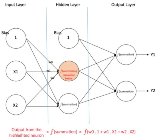
Artificial neural networks (ANNs) are algorithms that are modeled on neuronal structure of cerebral cortex of human brain, but on much smaller scales. A neural network (NN) structure is divided into different layers: the input layer, one or many hidden layers and the output layer. Each layer comprises of nodes or neurons. A basic unit of computation in neural network is a neuron, which receives an input from previous layer nodes along with their specific weights and perform a function on them. This function is also called the activation function. These neurons are activated by using different activated functions. Some examples of the activation functions include the sigmoid, tanh and Relu function. A bias is usually added with each layer to provide regularization and move the function graph by some constant from the center. The goal of the ANN’s is to decrease the loss function which is derived from the dataset. An example of mean square loss function used in the output layer is given by
𝐸(𝑦, 𝑦′) = 1
2||𝑦−𝑦
′||2 (1)
As compared to SVM which uses only one function, the neural network provides non-linearity due to its structure of layers. There are different types of neural net-works, for example feedforward NN, single layer perceptron, multi-layer perceptron 1 and so on. The output layer in case of classification usually consists of sigmoidal
ac-Figure 1: A multi-layer perceptron with one hidden layer
tivation function to provide probability for different classes or labels for the datasets.
3.2.2 Deep Neural Networks
They are differentiated from the basic neural networks by their depth; that is, the number of node layers through which data passes in a multi-step process of pat-tern recognition. In this each layer of network is supposed to learn specific features as received from the previous layers. The further the layer is, nodes are able to un-derstand more complex features, since they aggregate and recombine those features from previous layers. Deep-learning networks perform automatic feature extraction
without human intervention, unlike most traditional machine-learning algorithms.
3.2.3 Convolution Neural Networks
The idea behind Convolution Neural Networks(CNN) was derived from neural networks with neurons that learns from weights and biases. In this also each layer calculates a non-linear function using dot product and some activations. CNN’s work on the images itself in the input layer. The normal NN’s does not scale very well from the raw images because they are not able to learn enough features from them. The architecture of CNN’s introduced different types of layers which learns specific features from the previous layer. Thus in a generic idea the starting layers are able to learn more generic features such as the curves and edges from the images then as the architecture grows these layers becomes more specific, for example detecting the ears of an animal. Unlike a NN a CNN have neurons arranged in 3 dimensions namely width, height and depth. The depth here refers to the channels in an image, for a color image the depth is 3 whereas for a grayscale image it is 1. A ConvNet architecture is built from different type of layers which are repeated as necessary to build the deep ConvNet. These layers are:
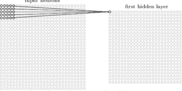
1. Convolutional Layer: The Convolution layer tries to learn the features from the images by preserving the spatial relationship between the pixels. It uses the concept of filters. On a broad idea the images are divided in small squares on which these filters are projected. These filters contains different values of pixels, for example a filter can be used to find edges of text in spam images. So, if there is such edges in the speculated square of images, those pixels are activated. The pixels on filter are multiplied on the input image area under consideration and a sum is performed over those activated pixels within the filter to check the
intensity of the filter. These filters work in sync with the depth of images, so if the image is RGB then there are 3 filters used for each depth of given sizes. There are three parameters that control the size of the Convolution layer. These are stride, depth and padding. The depth of the Convolution layer is mostly determined by the depth of the raw images or based on the previous layer input. The stride defines the number of pixels the filters are slided from left to right. Sometimes the input layer features are padded with zeros to maintain proportion with the size of the filter and to control the size of the output layer.After sliding the filter over all locations of input array we get an activation map or feature map. A Figure 2 below depicts an activation map generated from an image of 1 depth. The output dimension of a convolution layer is given by
𝑂= 𝑊 −𝐾+ 2𝑃
𝑆 + 1 (2)
where 𝑂 is output height or width, 𝑊 is the input height or width, 𝐾 is the filter size, 𝑃 is padding, and 𝑆 is the stride
2. RELU (Rectified Linear Units) Layer: To provide non-linearity after each Con-volution layer it is suggested to apply a RELU layer. A RELU layer works far better in terms of performance as compared to the sigmoid or tanh functions without compromising the accuracy. This layer also overcomes the problem of vanishing gradient. In vanishing gradient the lower layers train much slowly because the gradient due to back-propagation decreases exponentially through the layers. The RELU function is given as
Figure 2: Visualization of 5x5 filter convolving around input volume and producing activation map
This function changes all negative values to 0 and increases the non-linearity of the model without affecting the output of the Convolution layer.
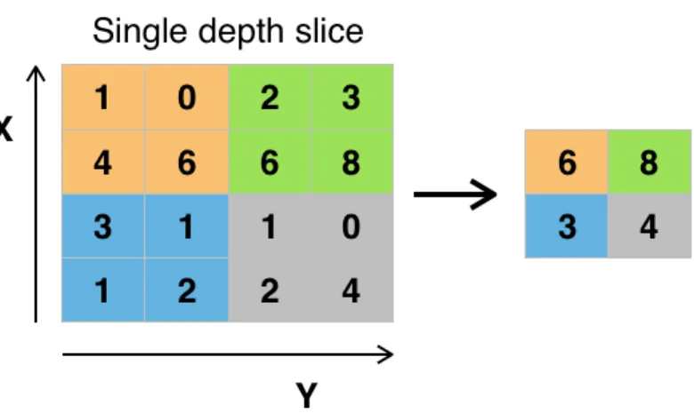
3. Pooling Layer: It is also known as the down-sampling layer. It uses a filter of given size, moves across the input from previous layer and applies a given function. For example in max pooling layer a max of all the filter values is given as output. There are other types of pooling layers as well such as average pooling and L2-norm pooling. This layer serves two purposes. One, it decreases the amount of computation by decreasing the amount of parameters of weights. It also overcomes overfitting in the model. The Figure 3 below shows the max pooling example.
4. Dropout layers: This layer helps in overcoming the problem of overfitting. Over-fitting means the weights and parameters are so tuned to the training examples after training the network, that they perform very bad on the new examples.
Figure 3: Maxpooling of 2x2 filter and a stride of 2
So this layer drops out a random set of activation in a given layer by setting there values to 0 [8].
5. Fully Connected Layer: This layer takes as input from any of the Convolu-tion layer, Pooling or RELU layer and outputs a N dimensional vector. This N depends on the number of classes you want to classify. In case of Spam classification the value of N = 2 i.e. weather the image is a SPAM or a HAM.
Thus a classic CNN architecture is composed of the above layers repeated in some fashion as necessary. A simple example of such architecture is given below 4.
Figure 4: A simple CNN architecture composed of different layers
3.2.4 Transfer Learning
Data is an essential part of deep learning community. As you train your net-works on large amount of data the network becomes more redundant and efficient in generalizing the results to new datasets. Thus in case you have a small amount of
dataset to actually work on, transfer learning overcomes this caveat. It is a process of using pre-trained models, which are trained on millions or billions of samples of generalized datasets and then fine-tune these models on your own datasets. Rather than training the whole network we use a pre-trained model weights and freeze them and focus on training only specific lower level of layers which are more specific to our dataset. If your dataset is different from the pre-trained model dataset then in that case training more layers of the model is preferred. This project focused on using two such pre-trained models VGG16 and VGG19.
A technique called data augmentation is widely used in overcome the problem of having less samples of dataset. It performs different image transformation on the images to produce new images and hence augment the dataset. Some transformations may include scaling the image by some ratio, rotating them, skewing, flipping and cropping the images.
3.3 Other Terminologies
This project also uses the following terms to quantify the results:
∙ True Positive (TP): The image is the SPAM image and classifier mark it is as a SPAM
∙ True Negative (TN): The image is the HAM image and classifier mark it is as a HAM
∙ False Positive (FP): The image is the HAM image and classifier mark it is as a SPAM
∙ False Negative (FN): The image is the SPAM image and classifier mark it is as a HAM
∙ Confusion Matrix: This is a matrix between TP, TN, FP and FN. A Figure 5 taken from [1] is shown below.
Figure 5: A Confusion Matrix [1]
∙ Accuracy: It is a metric used to determine how well a classifier works. It is defined as:
𝐴𝑐𝑐𝑢𝑟𝑎𝑐𝑦= 𝑇 𝑃 +𝑇 𝑁
𝑃 +𝑁 (4)
where P (Positive) = TP+FN and N (Negative) = TN+FP
∙ ROC and AUC: ROC (Receiver Operating characteristics) and (AUC) Area
under the Curve can be obtained from a trained classifier. A ROC curve is plotted against TPR (True positive rate) and FPR (False Positive rate) for varied threshold values. An area under this ROC curve is known as AUC value. TPR and FPR is determined as:
𝑇 𝑃 𝑅= 𝑇 𝑃
𝑃 =
𝑇 𝑃
𝑇 𝑃 +𝐹 𝑁 (5)
An AUC close to 1 for a classifier is considered as a good classifier.
∙ K-fold cross validation: In this technique the classifier is trained K times. The dataset is divided into K subsets. Each time a classifier is trained, one of the k subsets is used for the validation or test set and the remaining k-1 subsets are used for the training set. The accuracy over all these K classifiers is averaged to provide the average accuracy. Cross validation techniques are generally used to overcome over-fitting within the datasets.
∙ Stratified K-fold cross validation: It is a slight variation in the K-fold cross validation technique. In this each fold is created in such a fashion that each subset contains approximately same percentage of each target class. This is used in cases where the dataset classes are skewed i.e one class predominates the other.
CHAPTER 4 Related Work
Image spam detection can be done using various techniques. One such approach is to use content based detection i.e. to segment the content using OCR techniques and then classify it. Other approaches include to detect image spams based on the properties or features extracted from these images. Different machine learning algo-rithms are also used in conjunction with image processing to generate strong classi-fiers. Also deep learning techniques such as CNN can also be used on the raw images to detect image spams.
A content based image spam detection technique is discussed in [6] which uses OCR techniques on spam images. Then it extracts the text from the segmented image and perform textual analysis on the text to determine weather the image is spam or not. Another paper by Gevaryahu, Elias-Bachrach et al. [4] used the image meta data properties such as file size and other properties to detect spam images. The work presented in [9] used probabilistic boosting trees for classification by working on color and gradient histogram features and achieved an accuracy of 94%.
Sanjushree, Suhasini et al. [10] uses support vector machines and particle swarm optimizations (PSO) on ten metadata features and three textual features for image spam classification. Using the combination of these techniques they were able to achieve 90% accuracy on the Dredze dataset (discussed below) using 380 test and 300 training images. The authors of this [9] used cluster based filtering techniques using client and server based models and claimed to achieve 99% accuracy.
and they claim to have achieved an accuracy of 85%. Annadatha et al. [6] used linear SVM classifier on 21 image properties and each property was associate with a weight for classification. The author performed feature reduction and selection based on these weights. Two datasets [9] [4] was used by them and they achieved an accuracy of 97% and 99% on them. They also developed a new challenging dataset to challenge their classifier.
Aneri et al. [1] used 38 features extracted from Dredze and Image Spam hunter (ISH) datasets (discussed below) and used SVM kernels and achieved an accuracy of 97% with linear, 96% with RBF and 95% with polynomial kernel on ISH dataset and 98% using linear, 98% using RBF and 95% using polynomial kernel on Dredze dataset. They also used feature reduction techniques like univariate feature selection (UFS) and recursive feature elimination (RFE) to reduce the 38 features and provide better results. Expectation and Maximization (EM) clustering techniques was also used by them which did not performed well and achieved an accuracy of 87% on ISH and 70% on Dredze dataset. They also created a new challenging dataset which is also used in this paper, but were not able to provide good results for it 52%. This paper used Dredze, ISH and improved dataset for different techniques. The number of samples used in this project are relatively large from these datasets as a big part of this project also discusses the data processing techniques used to extract images from the spam archive, which was an unprocessed dataset provided by Dredze. Hence the amount of data the experiments and results are based on are large as compared to all previous papers so far in this domain.
Soranamageswari et al [12] used back-propagation neural network based on only color features and was able to achieve 92.82% accuracy. Another interesting aspect used in this paper was of splitting the image into different blocks and using them as
a feature, but they were only able to achieve 89.32% accuracy with this approach. Hong-Gang Zhang and Er-Xin Shang [13] used convolution neural networks to classify 7 categories of unwanted content embedded in images. The worked on a dataset containing around 52K images. The 7 categories targeted by them included commodities, spam images, political content images, adult content, recipe images , scenes and everything else. They used 5 convolution alongside max pooling layers. The output of these layers is given to the fully connected layer and a SVM classifier is used on this N sized feature vector. They resized all the images to 256x256 size and were able to achieve an average accuracy of 75.1% accuracy for the same. This project also used a custom CNN architecture, but only works on 2 categories classification that is SPAM and HAM.
CHAPTER 5 Framework
5.1 Datasets
This project uses 3 different datasets used by Aneri et al. [1]. However the number of images used in this project is much larger as compared to the images used in their paper. This project focused on making use of different formats of images such as gif, jpeg, jpg, png, tif and bmp. The gif images were processed and the first frame were extracted from gif images and converted to png files.
5.1.1 Dredze Dataset
Dredze et al. created a image spam archive dataset [4]. Dredze created a spam archive as well as a personalized spam images. Additional, the spam archive contained lot of unprocessed files in different formats such as gif, txt, jpg etc. We preprocessed this archive as well to augment our dataset. Then the experiments were performed on the combination of dredze spam archive and dredze personalized data set. Earlier papers [6] [1] focused only a subset of the personalized spam images. After prepro-cessing, the personalized spam images obtained were 3165 with 1760 HAM images and the spam archive images obtained were 10937.
5.1.2 Image Spam Hunter (ISH)
Image spam hunter dataset contained both ham and spam images [9]. We ex-tracted and processed 922 Spam and 820 Ham images.
5.1.3 Improved Dataset
This dataset was created by Aneri et al. [1]. This dataset was created by per-forming transformation on the ham images to make them look like spam. The ham images were resized to the size of spam images to align there metadata features. Noise was introduced in the spam images to make there edge detection difficult, since spam images generally have less noise as compared to ham images. These noise induced spam images were overlay on top of the ham images to generate the improved dataset. We experimented with 1030 improved spam images.
5.1.4 Combined dataset
Since we also used convolution neural networks for our experiments and in general CNN requires large amount of datasets to converge and perform better. So instead of experimenting with individual datasets mentioned above we combined together all these datasets to augment the number of spam samples. In order to account for the ham images we downloaded images belonging to different categories that are not spam to make our dataset balanced. Hence we were able to accumulate 11440 spam and 11267 ham images.
5.2 Data Pre-Processing
The Dredze dataset archive contained a lot of unwanted files and corrupted im-ages from which features could not be extracted. There were a lot of imim-ages in different formats and almost 60-70% of the images were in GIF formats. These gif images were processed to extract the first frame and then saved as a png format which helped in augmenting out dataset. The following steps in order to achieve this objective:
1. All unwanted formats such as .txt were removed.
2. All .gif images were converted to png files. All frames of the .gif images were extracted and first frame was saved as the spam image. The rest of the frames did not contained the spam image and were discarded.
3. All corrupted files were removed.
In order to achieve the above objectives, different proof of concepts were run. We created bash scripts to perform all above steps and keep track of the results after each step to get a clean augmented spam images.
5.3 Image Features
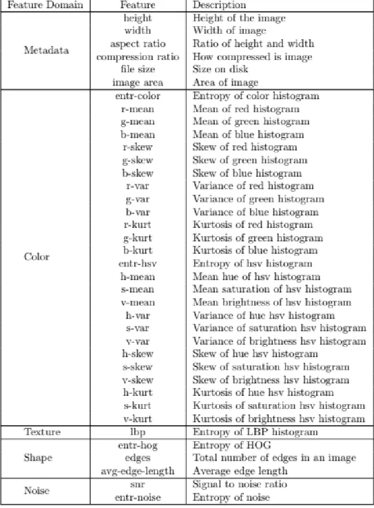
The first part of the experiments used neural networks and deep neural networks on features extracted from the images from different datasets as mentioned above. This project uses 38 features as mentioned in previous work [1]. The features are classified in 5 categories namely metadata, color, texture, shape and noise features. Figure 10 below describes the different features belonging to each categories taken from this paper [1]. The different categories of features is discussed below
5.3.1 Metadata Properties
These properties contain the image height, width, aspect ratio, bit depth and compression ration of the image files. Compression of an image is defined as
Compression Ratio= height*width*channels
5.3.2 Color Properties
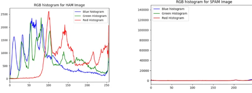
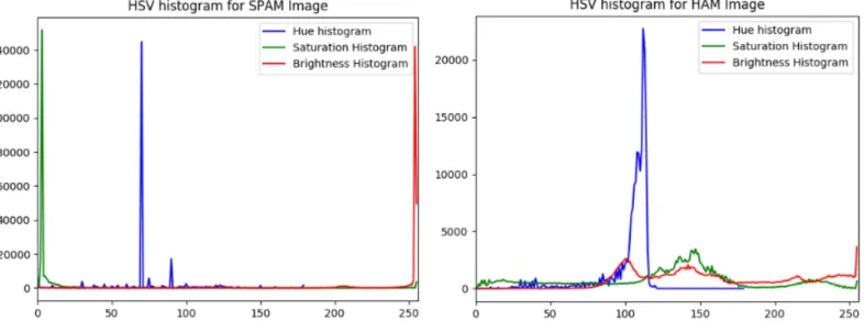
These properties include mean, skew, variance and entropy values of different properties of an image such as RGB colors, kurtosis, hue, brightness and saturation. Mean can be a basic color feature that represents the average pixel value of the image. That is, it is useful for determining an image background. A spam and a ham image has different histogram properties for these features as depicted in the Figure 6 below. These histograms shows the reasoning behind selecting these properties of color for classification. Similarly, Figure 7 below shows the histogram for HSV’s values of spam and ham images. In images, glossier surfaces has more positive skew values as compared to lighter and matte surfaces. Hence we can use skewness in making judgments about image surfaces. Kurtosis values are interpreted in combination with noise and resolution measurement. High kurtosis values goes hand in hand with low noise and low resolution. Spam images usually have high kurtosis values.
Figure 7: SPAM vs HAM HSV’s histogram
5.3.3 Texture Properties
The LBP (Local Binary Pattern) is used to determine similarity and information of adjacent pixels. The LBP would appear to be a strong feature for detecting image spam that is simply text set on a white background. In case of spam images these histograms will be having high intensity for specific values rather than being scattered.
5.3.4 Shape Properties
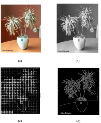
HOG (Histogram of Oriented Gradients) determines how intensity gradient changes in an image. HOG descriptors are mainly used to describe the structural shape and appearance of an object in an image, making them excellent descriptors for object classification. Edges are one of the most important features to detect spam images. They serves to highlight the boundaries in an image. Canny edge filters are used to find the edges. Figure 8 below shows the contrast in canny edges for spam
and ham images. Figure 8 and 9 shows the hog features for ham and spam images.
Figure 8: a) HAM original Image b) HAM Grayscale Image c) HAM HOG d) HAM Canny edges
Figure 9: a) SPAM original Image b) SPAM Grayscale c) SPAM HOG d) SPAM Canny edges
5.3.5 Noise Properties
These features include signal to noise ratio (SNR) and entropy of noise. Spam images tend to have lesser noise as compared to ham images. SNR is defined as the ratio of mean to standard deviation of an image.
Figure 10: Different Image Features
5.4 Techniques Used
5.4.1 Neural Networks
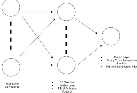
A back-propagation neural network with 1 hidden layer with 20 neurons was used. The input layer consisted of the 38 features as mentioned above . The hidden layer used the RELU activation function and the output layer consists of sigmoid activation function with one neuron. A K-fold stratified cross validation with K = 10 was used with this. An architecture of the model is shown in Figure 11.
Figure 11: NN Architecture
5.4.2 Deep Neural Networks
In this the simple neural network was extended to introduce another hidden layer with 10 neurons and with RELU activation function. Binary crossentropy was used as the loss function with K-fold stratified cross validation.
5.4.3 Convolution Neural Network
This project discusses two CNN architectures. We named it as CNN1 and CNN2. CNN1 was trained for 30 iterations whereas CNN2 was run with 25 iterations. Both of them was trained with a batch size of 64 images. The training set contained 19924 images whereas the validation set contained 2681 images.
5.4.3.1 CNN1 architecture
CNN1 architecture as defined below was used as the third model to draw results. The images were first rescaled to 128 x 128 x 3 and then fed to the network.
1. 96 filters of size 3 x 3 x 3 were used to the input layer with a stride of 1 followed by the rectilinear linear operator (RELU) function.
2. On the output of 96 x 126 x 126 from previous layer a max-pool layer is used taking the maximum value from a 3 x 3 area with stride of 2 x 2.
3. On the input of 96 x 62 x 62 from previous layer another convolution layer with 128 filters with 3 x 3 filter size and stride of 1 and no padding is used followed by a RELU activation function.
4. On 128 x 60 x 60 input from previous layer another maxpooling layer with a 3 x 3 area and stride of 2 is used on the input of previous layers to produce an output of size 128 x 29 x 29.
5. The input of previous layer is flattened and given to a fully connected layer. The N vector obtained from the input layer is of size 107648. On this N vector a dense layer of size 256 is used with RELU as activation function and a dropout
layer with probability of 0.1. Another dense layer of size 1 which acts as the output layer is added to the end of this with sigmoid activation function.
5.4.3.2 CNN2 architecture
The second CNN2 architecture is defined below, was used as the fourth model to draw results. The images were again first rescaled to 128 x 128 x 3 and then fed to the network.
1. 128 filters of size 3 x 6 x 6 were used to the input layer with a stride of 2 followed by the rectilinear linear operator (RELU) function.
2. On the output of 128 x 62 x 62 from previous layer a max-pool layer is used taking the maximum value from a 4 x 4 area with stride of 1.
3. On the input of 128 x 59 x 59 from previous layer another convolution layer with 128 filters with 4 x 4 filter size and stride of 1 and no padding is used followed by a RELU activation function.
4. On 128 x 56 x 56 input from previous layer another maxpooling layer with a 3 x 3 area and stride of 1 is used on the input of previous layers to produce an output of size 128 x 54 x 54.
5. On the previous layer input another convolution layer with 256 filters with 3 x 3 filter size and stride of 2 is used followed by a RELU activation function. 6. On 256 x 26 x 26 input from previous layer another maxpooling layer with a 5
x 5 area and stride of 2 is used on the input of previous layers to produce an output of size 256 x 12 x 12.
7. The input of previous layer is flattened and given to a fully connected layer. The N vector obtained from the input layer is of size 36864. On this N vector a dense layer of size 1024 is used with RELU as activation function and a dropout layer with probability of 0.2. Another dense layer of size 128 is added after that with a dropout layer with probability of 0.1 and RELU activation function. The final layer is of 1 neuron, which acts as the output layer with sigmoid activation function.
5.4.4 Transfer Learning
There are pre-trained models that are open sourced by some communities. These models are trained on billions of images such as ImageNet database [14]. Transfer learning is used to decrease the computation time to train your own network and to make you make use of these pre-trained networks. We can freeze some layers based on our requirements and only train a subset of those layers on our own dataset. There are two such pre-trained models available open source VGG16 and VGG19 [15] [16]. However this project only discusses the VGG19 model and the assumption is that VGG16 would have performed similar to VGG19 with some minute difference in accuracy.
5.4.4.1 VGG19
The architecture of VGG19 is described in Figure 12 below. We added 3 fully connected layers at the bottom with 1024, 512 and 1 layer respectively and added a dropout layer with probability of 0.3 with 1024 neurons layer. We freeze all the layers of the network and just trained this fully connected layer added to the end with 50 iterations.
CHAPTER 6 Experimental Results
As previously discussed SVM’s and EM clustering gave good results with features extracted from images [1]. We first discussed the neural network results, then we went deeper into the network and showed our results from deep neural network. Then we showed an alternative approach, of using raw images from our dataset and explained the results obtained from CNN1 and CNN2 architecture. Finally we concluded the results obtained from VGG19 model which uses transfer learning approach. All the following results were obtained from the datasets discussed in Chapter 5. Neural networks and deep neural networks were trained and tested on Dredze, ISH dataset and improved dataset. Whereas CNN1, CNN2 and VGG19 was run on the combined dataset.
6.1 Neural Network
We created a neural network with architecture discussed in Chapter 5 and ran it for Dredze, ISH and Improved Dataset.
6.1.1 Image Spam Hunter Dataset
The NN was run with 100 mini batch size and for 500 iterations with 10 fold stratified cross validation. The mean accuracy obtained after training the model was 99.07%. Below Figure 13 shows the AUC achieved by the best classifier over the whole ISH dataset and the confusion matrix obtained with 0.7 threshold value is shown in Figure 14 below. The FP rate obtained was 0.12%.
Figure 13: ROC curve for NN trained on ISH dataset
Figure 14: Confusion Matrix for ISH trained on NN
very low accuracy of 5.5%, which was expected as the improved dataset was meant to fool such classifiers. So in the next experiment the ISH dataset was combined with the improved dataset and then trained on the NN which gave an accuracy of 98.29% and an area under curve of 0.99. The ROC curve regarding the same is given below.
Figure 15: ROC curve for NN when trained on Improved dataset combined with ISH dataset
6.1.2 Dredze Dataset
The same NN was run on the personalized Dredze dataset and on Dredze spam archive combined with personalized dataset with 10 fold stratified cross validation. We got mean accuracy of 98.9% and 96.71% for both of them respectively. The ROC curve when the NN was run on Dredze spam archive combined with personalized dataset is shown in Figure 16 below alongside its confusion matrix. The FPR achieved in this case was 0.8%. When this model was tested on improved dataset we achieved an accuracy of 4.2%.
Figure 16: ROC & Confusion Matrix for Dredze dataset trained on NN When the whole Dredze dataset was combined with the improved dataset and then trained on the NN we achieved an accuracy of 94.42%. Figure 17 below shows the ROC curve obtained for the same experiment.
Figure 17: ROC curve for Dredze dataset combined with improved dataset on NN
The summary of all the results when trained with different combination of dataset on the NN is shown in Figure 18 below.
Figure 18: Summarized Result of NN trained on different datasets
As shown above, NN gave best results with ISH. It performed poorly when trained on ISH or Dredze dataset but when tested on improved dataset. However when the two datasets were combined with the improved dataset the NN was still able to perform better, however decreased the overall accuracy of other datasets as it acted as noise for them.
6.2 Deep Neural Network
The purpose of using a deep neural network was to compare the results obtained from the neural network above and see if introduction of extra hidden layers actually affect the results or not. In this case also the experiments were performed on the same datasets and their combination with improved dataset as done in previous section.
6.2.1 Image Spam Hunter
Two experiments were performed on the ISH with the same configuration as discussed in chapter 5. When the DNN was trained on ISH dataset alone we achieved a mean accuracy of 98.78%, an ROC curve and confusion matrix as shown in Figure 19 below. The FPR in this case was 0% and when this model was tested on the improved dataset we achieved an accuracy of 5.24%. When the DNN was trained on improved dataset combined with ISH dataset we achieved a mean accuracy of 98.13% and an ROC curve as shown in the Figure 20 below.
Figure 20: ROC curve for ISH dataset combined with improved dataset and trained on DNN
6.2.2 Dredze Dataset
The Dredze dataset was trained with the deep neural network architecture as discussed in Chapter 5. After training it on the personalized dataset we achieved an accuracy of 98.95%. When the same model was trained on the personalized combined with the spam archive we obtained an accuracy of 96.82% and a FPR of 1%. When this model was tested on improved dataset we achieved an accuracy of 5.9%. The ROC curve and confusion matrix obtained for the latter case is shown in Figure 21 below.
When the Dredze dataset was combined with the improved dataset we achieved the following ROC curve Figure 22 and a mean accuracy of 95.63%.
The summary of all the results when trained with different combination of dataset on the DNN is shown in Figure 23 below.
Figure 21: ROC & Confusion Matrix for Dredze dataset trained on DNN
Figure 22: ROC curve for Dredze dataset combined with improved dataset on DNN
the introduction of extra layer indeed increased the accuracies for Dredze dataset with more samples but decreased the accuracy of ISH dataset with comparable lesser samples. It also became more robust to the improved dataset.
Figure 23: Summarized Result of DNN trained on different datasets
6.3 Convolution Neural Network & Transfer Learning
We trained CNN1 and CNN2 architectures on 19924 images of spam and ham and tested on 2681 images. The CNN1, CNN2 and VGG19 were trained on a GPU machine with GeForce GTX 960M, Cuda Version 8.0 and compute capability - 5.0 configuration and each model took an average of 4 days to train. CNN1 was trained for 30, CNN2 for 25 iterations and VGG19 for 50 iterations. For all of these models adam optimizer was used along with binary cross-entropy. Figure 24 show the training
accuracy, training loss, validation accuracy and validation loss obtained over the 40 epochs the CNN1 model was trained.
Figure 24: Accuracy vs Loss for CNN1 model
Following Figure 25 shows the accuracy results for the three models when trained on the combined dataset and when tested on the improved dataset.
From the above table it can be concluded that as the CNN2 performed little bit better as compared to CNN1 as it had more layers. Also VGG19 performed better than the other two because it was a pre-trained model on a much larger dataset. Transfer learning hence is preferable in such scenarios when there is lesser time and resources available to train your own model.
CHAPTER 7
Conclusion & Future Work
In this project we make use of different real world image spam datasets and pro-vide strong classifiers based on neural network, deep neural network and convolution neural network. This project was able to provide better results as compared to the results presented by Aneri et al. [1]. These techniques were able to learn even from the improved dataset provided by them. However there is much more to this then meets the eye. Even tough it worked better there is a lot of margin for improvement. With the advent of deep learning which make use of big data available across the Internet, even more strong classifiers are feasible. Techniques like generative adversarial networks (GAN’s), introduced in year 2012 by Ian Goodfellow [17] can be used for this purpose. Using GAN’s which is based on Nash equilibrium, more stronger and robust classifiers can be built. Also, object segmentation using CNN and RNN (Recurrent Neural Networks) [18] can be used to detect the segmented region of spams and remove them from the images by extrapolating a background from ham images. Using such techniques, spam images can be converted to ham dynamically. Also, different experiments with different architectures within the CNN can be used to quantify different results. We can also use RFE (Recursive Feature Elimination) and UFS (Univariate Feature Selection), as done in the previous work [1] on the image features, when trained to neural networks and deep neural network to decrease the number of features under consideration.
LIST OF REFERENCES
[1] A. Chavda, “Image spam detection,” 2017. [Online]. Available: http:
//scholarworks.sjsu.edu/etd_projects/543/
[2] L. Whitney, “Report: Spam now 90 percent of all e-mail,” CNET News, vol. 26, 2009.
[3] C.-C. Lai and M.-C. Tsai, “An empirical performance comparison of machine learning methods for spam e-mail categorization,” inHybrid Intelligent Systems, 2004. HIS’04. Fourth International Conference on. IEEE, 2004, pp. 44–48. [4] M. Dredze, R. Gevaryahu, and A. Elias-Bachrach, “Learning fast classifiers for
image spam.” in CEAS, 2007, pp. 2007–487.
[5] M. Stamp, Information security: principles and practice. John Wiley & Sons, 2011.
[6] A. Annadatha and M. Stamp, “Image spam analysis and detection,” Journal of
Computer Virology and Hacking Techniques, 2016.
[7] S. Dhanaraj and V. Karthikeyani, “A study on e-mail image spam filtering tech-niques,” in Pattern Recognition, Informatics and Mobile Engineering (PRIME), 2013 International Conference on. IEEE, 2013, pp. 49–55.
[8] N. Srivastava, G. Hinton, A. Krizhevsky, I. Sutskever, and R. Salakhutdinov, “Dropout: A simple way to prevent neural networks from overfitting,” The Jour-nal of Machine Learning Research, vol. 15, no. 1, pp. 1929–1958, 2014.
[9] Y. Gao, M. Yang, X. Zhao, B. Pardo, Y. Wu, T. N. Pappas, and A. Choudhary, “Image spam hunter,” inAcoustics, Speech and Signal Processing, 2008. ICASSP 2008. IEEE International Conference on. IEEE, 2008, pp. 1765–1768.
[10] T. Kumaresan, S. Sanjushree, K. Suhasini, and C. Palanisamy, “Image spam filtering using support vector machine and particle swarm optimization,” Int. J. Comput. Appl, vol. 1, pp. 17–21, 2015.
[11] U. Jain and S. Dhavale, “Image spam detection technique based on fuzzy
infer-ence system,” Master’s Report, Department of Computer Engineering, Defense
[12] M. Soranamageswari and C. Meena, “Statistical feature extraction for classifica-tion of image spam using artificial neural networks,” in Machine Learning and Computing (ICMLC), 2010 Second International Conference on. IEEE, 2010, pp. 101–105.
[13] E.-X. Shang and H.-G. Zhang, “Image spam classification based on convolutional
neural network,” in Machine Learning and Cybernetics (ICMLC), 2016
Interna-tional Conference on, vol. 1. IEEE, 2016, pp. 398–403.
[14] A. Krizhevsky, I. Sutskever, and G. E. Hinton, “Imagenet classification with deep convolutional neural networks,” in Advances in neural information processing systems, 2012, pp. 1097–1105.
[15] K. He, X. Zhang, S. Ren, and J. Sun, “Delving deep into rectifiers: Surpassing human-level performance on imagenet classification,” inProceedings of the IEEE international conference on computer vision, 2015, pp. 1026–1034.
[16] J. Long, E. Shelhamer, and T. Darrell, “Fully convolutional networks for semantic
segmentation,” in Proceedings of the IEEE conference on computer vision and
pattern recognition, 2015, pp. 3431–3440.
[17] I. Goodfellow, J. Pouget-Abadie, M. Mirza, B. Xu, D. Warde-Farley, S. Ozair, A. Courville, and Y. Bengio, “Generative adversarial nets,” inAdvances in neural information processing systems, 2014, pp. 2672–2680.
[18] S. Zheng, S. Jayasumana, B. Romera-Paredes, V. Vineet, Z. Su, D. Du, C. Huang, and P. H. Torr, “Conditional random fields as recurrent neural networks,” in
Proceedings of the IEEE International Conference on Computer Vision, 2015, pp. 1529–1537.
![Figure 5: A Confusion Matrix [1]](https://thumb-us.123doks.com/thumbv2/123dok_us/9956252.2488184/23.918.315.656.219.479/figure-a-confusion-matrix.webp)