Predicting Customer Behaviour in the Web Hosting Industry - A Study in Mathematical Modelling

(1)

Predicting Customer Behaviour in the

Web Hosting Industry - A Study in

Mathematical Modelling

Maren Demuth

Bachelor Thesis

Autumn Term 2017

Academic Supervisor: Claus Führer Industrial Supervisor: Jon Pagh, One.com Examinator: Dragi Anevski

Lund University Centre for Mathematical Sciences Numerical Analysis

(2)

Abstract

Companies want to keep their customers. Especially, when they offer subscription based services instead of one time purchases. In the former case, if customers want to leave the company, they

need to cancel their subscription. This is calledcustomer churn.

On the example of One.com, a company that offers subscription based web hosting, a mathematical model is developed to predict customer churn, so that churn preventive measures can be taken. In particular, tree based statistical learning methods such as Decision Trees and Random Forests are applied to the customer dataset of One.com and it is observed that churn predictions are made with sufficient accuracy, given that the available dataset contains information that is explanatory of churn. Then both models, Decision Tree and Random Forest, successfully deliver results that can be used for churn preventive measures on the customer base of One.com.

(3)

Acknowledgements

I am thankful to my supervisors Claus Führer and Jon Pagh for all the time they spend on helping and teaching me.

Claus, I deeply appreciate your wisdom and guidance about life - not only mathematics - that you shared with me. It made me rethink my ideas and plans and gave me another perspective to consider. Thank you for being curious and motivated throughout the whole project. I enjoyed explaining you my thinking as much as listening to your stories about seemingly prehistoric technologies. Also, dankeschön for bearing with me when I could not find the right words in the right language and mixed it all together.

Jon, it is so much fun to work with you. I am in awe of your skill to present complicated information in a structured manner as well as at the right complexity level to any audience. Thank you for teaching me almost all I know about statistical learning concepts, being open-minded towards my ideas and thoughts and always having a witty comeback up your sleeve. Not only have you been an awesome mentor, but also a great colleague and I am happy to continue working with you on future projects.

Furthermore, I thank One.com for allowing me to write my thesis with them and making all necessary data and infrastructure available.

Thank you Lea Miko Versbach for providing me with your well-written Master thesis and helping me find other inspirations.

(4)

Introduction

In the Software as a Service industry subscription based products and packages are common. It is not necessary to buy an activation key for Microsoft Office any longer, simply subscribing to Office 365 enables the user to install any Microsoft Office product. This subscription typically renews itself automatically without the customer having to do anything. Instead, the act that has to be actively pursued is a cancellation of said subscription. Clearly, customers cancelling is not

desired by the companies offering such services. They wish to prevent so called customer churn,

i.e. customers cancelling their subscriptions and exactly that is the practical focus of this thesis. One.com is a company that offers web hosting. That is, a customer can order a subscription for a domain name and server storage space to create a website and e-mail accounts. Until the customer cancels the subscription, it is renewed automatically every year. Now, many people already possess a domain or e-mail accounts in some form which means that web hosting is considered to be a saturated market. Acquiring new customers is expensive and for that reason keeping customers is important, so One.com is interested in churn preventive methods. There exist methods such as offering a customer a win-back deal after they have cancelled or offering a discount on the next subscription year during the cancellation process. These methods however have a big drawback: they act only after the customer already decided to leave - that is often too late. Ideally, it is known long before, if a customer will churn or not, so that preventive measures can be taken in time. But who knows the future?

Knowing the future is often described as a very ominous process and involves magical spectacles, so this is not what this thesis is about. Instead, the focus lies on a much smaller fraction of that question. First, only the future of the customer base of One.com is of interest and second, the only event that is going to be investigated is the one of them renewing their subscription or not. With those two heavy limitations on the future, it might actually be possible to predict it accurately.

For such prediction of customer churn a mathematical model is developed, which makes this thesis an exercise in mathematical modelling. In particular, statistical learning methods are used and it is the goal of the model to output a prediction for each customer, if she/he will cancel the subscription within the next time period or not, based on the information that is available for that customer.

To develop such a model this thesis first lays out the principles of mathematical modelling in Chapter 1. These are then inherited by the statistical learning models described in Chapter 2 and build upon to further specify the model. In the first two chapters a focus lies on establishing a theoretical background that gives a direction and points out important aspects for building a model. These aspects are then discussed in each following chapter. Chapter 3 introduces the concrete method used for predicting customer churn based on the previously introduced theory, while Chapter 4 describes application of this method to build the churn model and discusses the obtained results. In the last chapter, Chapter 5, further practical details of the model are given and the theoretical frame is closed.

(6)

1 Principles of Mathematical Modelling

1.1 Defining a Mathematical Model

The idea of modelling is very intuitive. Real-world phenomena are often too complex to be understood in their entirety. Instead, it is the aim to find simpler approaches to describe them. This is common to many disciplines not only mathematics. For example when drawing or painting

Figure 1: A Mannequin artists sometimes use wooden mannequins to understand human

stature and movement. Those mannequins are in no way humans, they differ in most obviously size and material, but they preserve important information about human body proportions and possible movements, e.g. it is not possible to bend the elbow of a mannequin backwards the same way it is not possible for a human.

It therefore seems that it is an intrinsic property of a model to represent reality, but only partially or in a simplified manner. Rutherford Aris states here that a model is a change of scale of the real world. When describing a physical object with a mathematical model the change of scale occurs on the axis of abstraction. [1,

p. 1f] He introduces the terminology prototype to describe what

has been called “real world” in this text, i.e. the prototype is the

observation or system that is investigated. A mathematical model

is according to him just the system of equations that describes the

prototype. Themodel theorythen represents the underlying assumptions and axioms of the system

of equations. This is based on the logician Alfred Tarski’s definition of a model, “A possible

realization in which all valid sentences of a theoryT are satisfied is called a model ofT.” [1, p. 2]

The change of scale on the axis of abstraction can be interpreted as changing from a linguistic description of the prototype to using mathematical language to describe it. The level of abstraction could then be the amount of detail incorporated in the model, i.e. a less detailed description corresponds to a higher level of abstraction and vice versa. This is picked up by John Maynard Smith in [1, p. 3]. He differentiates between the purpose for which a model is made. If it is a

practical purpose, he calls the mathematical description of a prototype a simulation. According

to him simulations increase in value by the amount of detail they incorporate. Note that the notion of value is not yet defined, but shall be discussed in a later chapter. On the other hand, if the mathematical description serves a theoretical purpose, he calls it a model. The latter should include as little detail as possible to be of value. For example, if it is the task to predict the population growth of a bacteria sample, then knowing its circumstantial growth rate and initial population size is crucial for valuable results. However, for descriptions of population growth of different species such details are not beneficial. Excluding them and instead defining the type of growth, e.g. exponential or logistic, increases the value of the description in that sense that it is not bound to a particular species. Hence the purpose of a model is important for its evaluation. This shall be discussed in more detail in the following chapters. This chapter concludes with the definition of a mathematical model Rutherford Aris states in [1, p. 5].

Definition 1.1. A system of equations Σ is said to be a model of the prototypical systemS, if it

is formulated to express the laws ofS and its solution is intended to represent some aspect of the

(7)

This definition refines the statement from the beginning and hints at the goal of mathematical modelling. In particular, a model needs to preserve qualities of the prototype in order to be valuable for drawing conclusions about it.

1.2 The Modelling Process

Just from the definition of a mathematical model it is hardly possible to actually build one. It is helpful to consider important steps of the modelling process such as the ones described by James Caldwell and Yitshak M. Ram. in [5, p. 3f]. They divide the process into seven steps which go from defining the situation at hand, i.e. understanding the prototype, to describing it as a mathematical problem which shall then be solved. The last step is to evaluate the model and in case the results are not satisfactory, the process has to be reiterated. In particular this leads to the following steps: 1. Specification of the prototype. In this step the real world situation has to be analysed

and understood. The model expectation needs to be defined and a goal formulated by which the model can be judged in the end.

2. Model set-up. Here it needs to be evaluated which features of the prototype should be

included in the model and which can be disregarded. This leads to defining the assumptions that the model makes.

3. Formulating the mathematical problem. Caldwell and Ram consider this the hardest

step. It is the goal to translate the linguistic description of the prototype into mathematical language. That includes assigning mathematical symbols to variables and deciding about their proportionality relationships.

4. Solving the mathematical problem. This step includes finding the solution to the

problem stated in Stage 3. To do so, it is necessary to decide upon a method of solution. Questions to be asked are, for example, if an approximative solution is sufficient? Shall the problem be solved numerically or analytically?

5. Interpretation of the solution. Here it needs to be assessed, if the model is behaving

reasonably. Also model accuracy and the behaviour of the model under changing conditions are considered.

6. Comparison with reality. This step is closely related to the previous one. If the results in

Step 5 do not compare well with reality, the modelling process needs to be reiterated starting at Step 1.

7. Completion of modelling process. If in Step 6 a satisfactory result has been obtained,

the modelling process can be considered as finished.

Many methods on solving mathematical problems already exist. Which ones where used in the practical part of this thesis will be discussed at a later point. However the more interesting part for now is the model evaluation of Step 5 and 6 for which general methods do not seem to exist. This is discussed in more detail in the next section.

(8)

1.3 Evaluating a Mathematical Model

In the previous chapters many terms have been used that were not yet well defined. For example, what is an accurate model? How do we measure accuracy? What makes a model valuable? Unfortunately, it does not seem like there exists a general theory on mathematical model evaluation, so it is not possible to answer all these questions at this point. Instead, it is the aim here to structure them and give an overview of what needs to be considered when evaluating a mathematical model.

1.3.1 Quality Characteristics

This section aims at defining quality characteristics that need to be considered in the model

evaluation. These can be split into a quantitative and a qualitative evaluation. For the quantitative aspects model accuracy and model complexity are considered. The big questions behind model accuracy is: How well does the model compare to reality? Clearly, this calls for some kind of metric that captures the differences between prototype and model, which is why accuracy is part of the quantitative evaluation. Note here that it is difficult to chose the right metric. For example when modelling the path a ship has to take to safely arrive in a harbour. Is it more important that the calculated velocity compares well to the actual values or that the modelled trajectory is accurate? Of course both have to be considered, but it might be that one accuracy measure performs well while the other one does not. Is the model still accurate then? Questions like these will be discussed in more detail later on.

On the same note model complexity requires a measure as well. And again, there is no one absolute truth here. It seems to be even harder to find a measure for model complexity than accuracy. In [1, p. 19] Aris hints that model complexity increases, if the equations that describe a model become more advanced, e.g. going from simple algebraic equations to partial differential equations. On the other hand in [11, p. 222] model complexity refers to a tuning parameter that allows for a dynamic adaptation to fit the problem. What both ideas have in common is that model complexity is related to the properties of the model equations, might it be the number of parameters used or the type of equation.

In contrast to the quantitative part stands the qualitative evaluation. Here points of interest are the purpose of the model, its limitations and considerations. The purpose describes the goal and background: Why is the model created and what shall the model achieve? As mentioned in 1.1 it is important for the evaluation to know the model purpose, because simply put: a fish should not be judged by its ability to climb a tree. Similar to the way that a fish is made to swim in water, a model is build for a particular propose and under certain conditions. It is not possible to then judge the model by its ability to perform tasks in a different environment.

The limitations refer to questions such as: When does the model apply and when not? What are the extrapolation powers of the model? Do the assumptions reflect reality sufficiently? This is answered at a later point. Lastly, the considerations leave room for discussion on special cases that have not been included before and practical problems such as computational power.

All in all there is a lot of points that need to be considered when evaluating and building a model. Many questions are left open at this point, since it requires further specification to answer them. Some might only be answered in the end, but in general each chapter of this thesis concludes with the part of evaluation that is possible at the respective step. The next two sections strive to start answering some questions and give more thorough definitions of terminology for which such definitions are missing at this point.

(9)

1.3.2 Comparison to Reality

The essential part of a model is to reflect a prototype in some way. Ideally, that reflection corresponds closely to observations of the prototype. This quality of correspondence is what has been called model accuracy in this text. In many sources accuracy is discussed only on a case by case basis due to the mentioned lack of a general theory. This however makes sense considering the argument above that models need to be judged on the background of their purpose.

As an example, in [1, p. 126] Aris describes the accuracy of a simulation (in Smith’s sense) as being easily obtained by a mere comparison between the predictions of the simulation and the observations of the prototype. If the agreement is good, then the model is of high accuracy. Furthermore, for the comparison of observation and prediction it is necessary to define a measure for the model that represents some attribute of the prototype. [1, p. 224]

He omits to give such statement about Smith’s model which further supports the conclusion of a lack of general theory. Furthermore, Aris discusses the complexity only of a simulation and not of a theoretical model as well. According to him a simulation is of good quality, if its complexity is low, i.e. the simulation is fit to the data by only adjusting few parameters. If these parameters are determined independently of each other and entered to the model as fixed constants, the simulation becomes even better. [1, p. 126]

In the previous section it was mentioned that model complexity relates to the properties of the model equations. There are different understandings of this term, but for this thesis complexity is understood as a tuning parameter that has to be determined for every model. This parameter could be a scalar for some penalty term that is introduced in the model or simply the number of basis

functions of a chosen function space. [11, p. 37] As an example consider n data points in R2 for

which a polynomial of degreem is fit. It is easy to find the interpolating polynomial that will have

at most degreem=n−1. The fit of this polynomial to thendata points will be perfect. However,

a model should not only explain given data points. When further data points are obtained, it is the aim that the model still describes these sufficiently well. The interpolating polynomial for some data points typically performs poorly on new data points that it was not fitted to previously. While

a polynomial of degree m < n−1 would fit the n data points worse, it is likely that it would fit

the new data points better. So by changing m the fit of the model can be adjusted which is why

m can be understood as the tuning parameter and a measure of complexity.

Both model accuracy and model complexity are important parameters to consider for the model evaluation and are discussed more thoroughly throughout the thesis.

1.3.3 Model Scope

Model scope is the chosen name for the qualitative evaluation as it summarises the important points of interest which are purpose, limitations, and considerations. Many times in the previous chapters it has been mentioned that most models cannot be viewed independent of their purpose and background. This is given a more thorough argument here.

When evaluating a model, it is always necessary to revise the underlying ideas and origins. [1, p. 22] If a model was build to predict the salary of football players based on their years of experience and games played, this model should not be judged upon its ability to present salary distributions across all professions as it certainly would perform worse with the latter task.

Aris differentiates between two main backgrounds of evaluation. Those closely relate to Smith’s distinction between a theoretical model and the more practical simulation. The latter is used to

(10)

gain an actual understanding of a particular prototype, e.g. when investigating the growth of a

bacteria sample. Whereas the first serves to gain conceptual progress, i.e. when it is the goal to

develop a theory that can be applied to different prototypes. Both backgrounds go hand in hand during the modelling process. Indeed it seems like there is a fluctuating relationship. The first two steps described in 1.2 are called “preliminary ideas” and “first model” by Aris. Those are closely related to the conceptual progress, since they build the theoretical backbone of the model. This stands in contrast to Step 3 and 4, “design of experiment” and “experience”. Those steps involve a solution to the particular problem at hand, which means a gain in actual understanding. Further down the line in the evaluation and interpretation of Step 5 and 6, the direction goes back to the conceptual progress, since from the interpretation of the solution revised mostly theoretical ideas emerge. This then concludes the circle back to Step 1.

Depending on the purpose of the model the modelling process “converges” to the corresponding background. That is, the modelling process can be thought of as following a fluctuating curve between actual understanding and conceptual progress which will converge to either side depending on the purpose. For a simulation ideally the actual understanding increases and for a model the conceptual progress. This differentiation has to be considered when the model is evaluated. [1, p. 22f]

The purpose of the churn model is identified in the next chapter which will make further evaluation possible, while the limitations of the churn model have to wait, until assumptions are stated at a later point.

1.4 Model Classification

As a first step on the way to classify the problem of customer churn, following Step 1 of the modelling process, it is discussed whether the model to be build is a simulation or a model in Smith’ sense. To recall, a simulation generally serves a practical purpose while the model has a theoretical ambition. It is not the focus of this thesis to develop a theory on general customer behaviour, but to be much more concrete and predict, if customers will cancel their subscription. This has the simple practical purpose of retaining customers which suggests that this thesis aims to build a simulation in Smith’ sense. Additionally, as can be seen in a later chapter, if the amount of relevant customer information is increased, the higher the accuracy of the prediction which is another attribute of a simulation. Hence, the churn model is a simulation and evaluation characteristics described in 1.3.2 apply.

Note that while having the classification as a simulation in mind, this thesis will refer to it as a model and not follow Smith’ distinction, unless explicitly stated.

Another important distinction to make is that the problem of customer churn is stochastic in nature. That is mostly because there are few to no deterministic relations in human behaviour. Why did a customer create 5 email accounts instead of 4? That might be because she or he has 5 family members, but it also might be because she/he felt like it that day. Most of the variables in the customer information are subject to random influence such as a customer’s mood or circumstance which are not measurable in this context. It is certain which amount of email accounts a customer can create, but not which amount a particular customer will create. The information for a customer is therefore described by a random vector for which each element is a random variable that describes a particular attribute to that customer. But not only the customer information is random, also the churn label in itself. This is because of the following reasons described in [12, p. 654].

(11)

• Data generation is subject to label noise. For instance it might be that a customer that

cancelled the subscription regrets the cancellation. In the data set the customer would be marked as having churned while that is not actually the case. A similar situation also occurs when a customer wants to change the domain name. As a domain name needs to be registered with an external organisation, it cannot simply be changed and as a consequence the customer needs to cancel his subscription and order a new one. Which means the customer is labelled as “churn” even though he/she actually stayed.

• Non-unique labels. In this case it is not possible to assign a unique label Y to an input

X = x0. For example, if it were the task to predict gender based on height, then a height

of x0 = 1.80 m can be the label “male” or “female”. Similarly if customers are described

by a fixed amount of variables, it might be that two customers share the exact same values for each variable while at the same time one customer will have churned, but the other one stayed.

Besides these random effects there are a few deterministic effects as well. For example will introducing a new product or removing an existing one affect which products are sold. Compared to the stochastic effects however, the influence of the deterministic effects is not as big. This is why the churn model is a stochastic model and in particular it is a statistical learning model. That means that deterministic effects are not considered which results in limitations of the model. These are discussed at a later point.

(12)

2 Statistical Learning Models

After introducing first concepts and classifying the problem of customer churn, which corresponds to Step 1 of the modelling process described in 1.2, this chapter aims to continue with the next steps of building a mathematical framework and formulating a concrete problem.

The basic idea of statistical learning theory assumes that there are certain relationships between data points that can be investigated to gain knowledge from large amounts of data. Those data points usually contain input and output values, i.e. for a given input value the prototype gives a corresponding output value. Often the relationship between input and output is complex and can hardly be detected by humans, so it requires more advanced statistical methods and tools as well as computational power to gain insights.

There are two distinctions to those methods, supervised and unsupervised learning. In the case

of supervised learning both input and output data sets of the prototype are available and are used to train a model. This is done by providing the model algorithm with a training dataset that

contains input and output. The algorithm then fits the model to the training dataset by learning patterns that it observes in the data. However, output data might not always be available and in that case the learning method is called unsupervised. Those models are much more difficult to build and evaluate, since the dataset basically does not contain any “answers” from which learning could be possible. [6, p. 26] Luckily, the problem of customer churn can be solved with supervised learning, since output data is available for each observation.

As it is typical with rather young scientific fields, there exist many terms for the same concept.

For example the input data is often called features, predictors orindependent variables while the

output data is referred to as responses,dependent or target variables. [11, p. 9] This text mostly

uses the term feature for input variables and prediction for output variables.

Depending on the situation it can be interesting to either thoroughly investigate the relationship between data points of a prototype or on the other hand predict an attribute of the prototype based on some given data points. For both situations a mathematical model is developed, but the focus

of each differs. The first is called interference where the relationship of input and output is of

interested, e.g. to understand how output data changes depending on some input data. The

latter is called prediction and here it is interesting to predict outputs based on some features.

Building a mathematical model for either case requires estimation of the relationship between input and output data, but only interference requires an explicit formulation of the relationship. For prediction purposes it suffices to implicitly know the relationship as long as it gives accurate

results. A prediction model where this is the case is also called black-box model. [6, p. 17 ff] Since

the churn model is clearly a predictive model the following discussion is focussing on those.

2.1 Classification versus Regression

The input and output data can be of two different forms, either quantitative or qualitative. In

the first case the variables are continuous, while for the latter case the variables are categorical or discrete. Integers are a special case in the context of statistical learning. Though they take numeric values and can be considered as quantitative variables, they can also represent labels of a categorical variable due to their discrete nature.

While the input dataset can be of mixed variable types, the type of output variables defines the name of the prediction method. When a quantitative variable is predicted, the prediction

(13)

classification. Again there exist many terms for qualitative variables, most often the possible values

of a qualitative variable are called classesor labels. [11, p. 9f]

For the problem of customer churn the target variable is not only categorical but also binary, a customer either cancels the subscription or not, which means that the churn model is a binary classification model.

2.2 Mathematical Set-up and Assumptions

To quote Rutherford Aris again, in [1, p. 39] he states that, if a type of model has been chosen, then “the formulation [of a model] is nothing more than a rational accounting for the various factors that enter the picture in accordance with the hypotheses that have been laid down.” This section shall try to achieve that, also following Step 2 of the modelling process described in chapter 1.2. In particular, this section deals with the general mathematical set-up for a binary classification problem.

Consider a set of input values X and a set of output values Y. Then all observations x of a

random variable X lie in X, i.e. X takes values in X. Similarly y is an observation of random

variableY which takes values inY. The points (x1, y1), . . . ,(xN, yN)∈X ×Y areN observations

of the pairs of random variables (X1, Y1), . . . ,(XN, YN) and build a training sample from which the

algorithm is supposed to learn.

Set Fall to be the set of all measurable functions between X and Y. It is the task of

classification problems to find a mapping f : X → Y with f ∈ F_all such that ∀x ∈ X the

number of wrongly assigned labels y is as small as possible. [12, p. 652] Note that the “wrong

assignment” means that the prediction does not correspond to the observation.

In this particular case of binary classificationY ={0,1}holds and typically it is assumed that

X ⊂ IRp where p is the number of features. It is possible however that X contains categorical

features. For example, if it were the task to predict, if a patient has a disease or not, then the doctor

might gather p= 3 points of information about the patient such as age, gender and symptoms of

that particular disease. For patient 0 this information is stored as the vectorx0 = [32,“female”,1]

where the latter 1 stands for positively identified symptoms. The prediction for this patient can

then either be y0 = 1 in which case the patient has the disease ory0 = 0 when she does not.

There is no assumptions on X and Y in particular. However, it is assumed that there exists

a joint probability distribution function P on X ×Y. Note that formally X ×Y needs to be a

σ-algebra in order for P to be defined as a probability distribution. However, in light of the scope

of this thesis and the fact that the underlying set of outcomes Ω is simply assumed to exist without

any further specifications, the setX×Y is assumed to have the necessary properties of aσ-algebra.

P can be any probability distribution and is unknown at the time of learning. Furthermore,P is

assumed to be fixed, i.e. it does not change over time.

It is also assumed that the points (Xi, Yi) for i = 1, . . . , N are independently sampled from

P and that the values in X and Y are non-deterministic, because of the previously mentioned

reasons, compare chapter 1.4. Due to the stochastic labels the conditional probability

η(x) :=P(Y = 1|X =x)

is considered. The composite beingP(Y = 0|X =x) = 1−η(x). If the non-deterministic effect

of the labels is small, η(x) will be close to 0 or 1 respectively, which is the desired situation for

statistical learning. However, if η(x) is close to 1₂, then the learning algorithm will make more

(14)

2.3 Bias-Variance Trade-Off

This section builds upon the mathematical set-up and aims to formulate the general consideration of statistical learning models in accordance with Step 3 of the modelling process described in Chapter 1.2.

In the previous section the mapping f :X →Y was introduced and it was established that it

is the goal to find the optimal f, i.e. the f that leads to the least amount of misclassifications. f

is called aclassifier.

In order to find such an optimal classifier it is necessary to define a measure for misclassifications.

This is done in [12, p. 656] by introducing a loss function L(Y, f(X)). A loss function can have

many forms, most commonly the squared error lossL(Y, f(X)) = (Y−f(X))2in regression settings.

However in the case of binary classification typically the misclassification error is used. The error

at some point (X, Y) is given by

L(Y, f(X)) =

(

1 iff(X)6=Y

0 otherwise

Ideally the loss function over a whole dataset (x1, y1), . . . ,(xN, yN) is very small. When the dataset

is labelled, i.e. the yi are known, then evaluation of the loss function is easy. However when a

dataset without labels is evaluated, a more advanced measure is necessary. In [11, p. 18] this

criterion is called the expected prediction error and in other sources risk. It is defined as

EP E(f) := E [L(Y, f(X))]

which is the expected loss of classifier f for inputX. [12, p. 656] It is then possible to define the

best classifier f∗ ∈F, whereF ⊂Fall, as the one for which

EP E(f∗)< EP E(f) , ∀f ∈F

In particular the notation f_F∗ is used to denote the best classifier in F, i.e.

f_F∗ := argmin

f∈_F

EP E(f)

IfF =Fall, then the best classifier is the Bayes classifier,

fBayes(x) :=

(

1 ifη(x)≥ 1 2

0 otherwise

So using the Bayes classifier for any binary classification gives the best results. Unfortunately, the

Bayes classifier cannot be used in practise, since the distribution P is unknown. Instead it is the

goal to construct a classifier f for which EP E(f) is as close as possible to EP E(fBayes). The

general problem of binary classification can be summarised as follows.

The problem of binary classification. Given independent, identical distributed (i.i.d.)

training points (X1, Y1), . . . ,(XN, YN) drawn from an unknown probability distributionP onX×Y

with loss function L, it is the goal to find a classifierf :X →Y for which EP E(f) is as close as

(15)

The optimal classifier in Fall is, as mentioned before, fBayes. Consider a subset F ⊂ Fall

that does not contain fBayes as this classifier is not usable in practise. The idea is to choose a

classifier whose expected prediction error is as close as possible to the expected prediction error of the Bayes classifier. The “closeness” can be evaluated through their difference that can be expanded the following way,

EP E(f)−EP E(fBayes) =EP E(f)−EP E(f_F∗ ) | {z } Variance +EP E(f_F∗ )−EP E(fBayes) | {z } Bias (1)

The variance, also calledestimation error, is the uncertainty introduced by randomly sampling n

training points. That is, given any finite sample the error of estimating f_F∗ by f is the estimation

error. On the other hand the bias (orapproximation error) is the error that occurs by approximating

fBayes by f_F∗. Depending on the F that is picked and consequently which f_F∗ is obtained, the

variance and bias change. If F is rather small, i.e. it only contains a few elements of Fall, the

bias tends to be big, since it is less likely that f_F∗ is close to the Bayes classifier. At the same time

the variance is small as it is more likely that the chosen f estimates f_F∗ well and vice versa. [12,

p. 662] Thus,F serves as measure for model complexity, since it is a tuning parameter, although

without an explicit form at this point.

Both variance and bias are non-negative, so to minimize (1) both need to be minimised at the

same time. As can be seen however, they have an inverse relationship. As the size ofF increases,

so does the variance, but the bias decreases. It is the holy grail of statistical learning to chose the

right F that contains a classifier for which the sum of bias and variance is minimised. Hence the

title of this chapter, the “Bias-variance trade-off”.

2.4 Evaluation

It has been promised in the first discussion of model evaluation that qualitative considerations and limitations will be picked up in later chapters. At this point, first statements on limitations can be

made. The assumptions on the probability distributionP in section 2.2 lead to two considerations.

First, the fact that P is assumed to be fixed implies that the model does not adapt to changes

of One.com over time. This is already mentioned in 1.4 where the example of introducing or removing products is given. Another example is a negative article about One.com in the media. To adapt to such changes, it is necessary to retrain the churn model when influencers change. Now the second consideration is a bit weaker, since it probably does not occur frequently, but the fact that independent sampling of the dataset is assumed, i.e. the information of each customer is independent of the other customers, does not completely correspond to reality, since customers simply might know each other or have read the same reviews of One.com.

Besides this short addendum to the model scope there is a bigger question of the quantitative discussion that is answered in the next section.

2.4.1 Model Accuracy

It is the aim of this section to consider the model accuracy orquality of fit for statistical learning

methods. There exist two different settings for which model accuracy is relevant. First, model

selection which is the process of deciding which model to use for the given prototype. To decide

upon a model, the performance of different models is evaluated and the best one is chosen. [11, p. 222] Note however that it might not be sufficient to simply compare models based upon their

(16)

better fit, since there might not be a significant difference. Instead, qualitative differences in the behaviour of the models have to be considered for the model selection as well. [1, p. 127] The second setting is more interesting for the context of this thesis and deals with the quantitative

evaluation of the chosen model. This is calledmodel assessment.

For both settings the model accuracy is obtained by estimating the expected prediction error. When a big data set is available, it is rather simple to find an estimate by splitting the data set into two parts: a training set and a test set. Typically the training set will be around 75% of the data while the test set takes 25%. The training set is then used to train the model and with the test set the expected prediction error is estimated by using a loss function. Though easy to implement, evaluating expected prediction error based on only one test set means that results can change significantly when a different test set is used to evaluate accuracy. To counteract the variability

re-sampling methods like k-fold cross-validation can be used. The idea there is to randomly split

the dataset intok subsets (“folds”) each of roughly equal size and treat one subset as the test set

while the remainingk−1 subsets serve as the training set. This is then iteratedktimes where each

time another subset serves as the test set and the resulting estimations of expected prediction error are averaged to give one final estimation which is typically more stable than the simple train/test split. [6, p. 177ff]

Besides re-sampling methods, there are analytical methods for model evaluation as well, e.g. minimum description length or AIC (Akaike information criterion). Those are not discussed here, since they are either not applicable or outside of the scope of this thesis.

For the estimation of expected prediction error a loss function L needs to be chosen, since

EP E(f) := E [L(Y, f(X))]. In this thesis that is the misclassification error introduced in Chapter

2.3. EP E(f) is then estimated by the sample mean of the test data setTtestwithNtestobservations.

When cross-validation is used, the test set is one of the previously split subsets in each iteration.

Using the training set would result in a too optimistic estimation, since the classifier f is fitted

using the data points from the this set. The sample mean is given by ¯ Ls= 1 Ntest Ntest X i=1 L(yi, f(xi))

∀i: (xi, yi)∈Ttest. For sufficiently bigNtestthis gives a good estimation of EP E(f), since by the

Law of Large Numbers the mean of i.i.d. random variables X1, . . . , XN each with expectation µ

converges toµ asN → ∞.

To measure the accuracy of the model it is then possible to evaluate

1−L¯s= Number of correct predictions

Ntest

However, this is likely to be a too optimistic estimate, since often in a classification problem the class sizes are unbalanced. In particular, in the churn example there is much more customers that stay than those that leave, so the model can happily predict customers that stay and miss most of the churners while an accuracy score as the one above would still be very high, since so many stayers are identified correctly.

Another problem with such a simple accuracy score is that it does not account for the different

types of errors, the type-I error andtype-II error. The type-I error, also calledfalse positive is the

error of rejecting a null hypothesis when it is actually true. Typically the null hypothesis is the

(17)

The type-II error (or false negative) denotes the error of not rejecting H0 when the alternative

hypothesis is true. [2] It is important to differentiate between those two error types, because they often have different consequences, for example for a model that predicts heart attacks. A type-II error, i.e. predicting that the patient will not have a heart attack while the opposite is true, is probably worse than a type-I error where the model predicts a heart attack when the patient is not going to have one. [11, p. 310] Of course there is other issues with type-I errors in medical settings such as administrating medications that are not necessary. This is however a complex topic and luckily this thesis just concerns itself with customer churn. For the churn prediction a type-II error is not that dramatic. Even though a churning customer is missed and wrongly predicted to stay, this has no direct negative impact considering that without the model none of the churners would be identified. A type-I error however might give the customer an incentive to churn when she or he actually planned to stay, if churn preventive measures such as a direct call or e-mail offers were not appreciated by the customer.

In conclusion, a pure misclassification error count is too simplistic. In order to differentiate

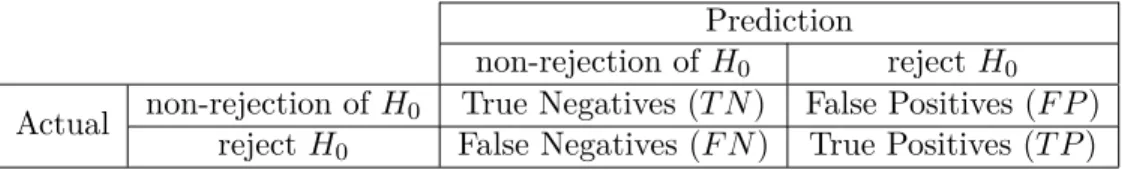
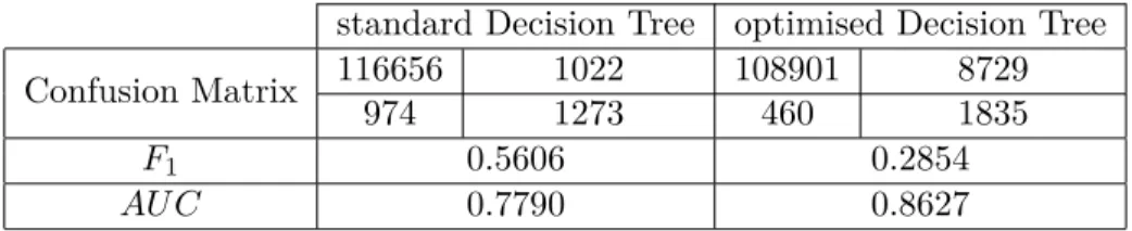
between type-I and type-II error theconfusion matrix is introduced. For a test data set the number

of type-I errors, type-II errors and correct predictions are counted and arranged as in Table 1. Table 1: Confusion matrix for a binary classification problem

Prediction

non-rejection ofH0 rejectH0

Actual non-rejection ofH0 True Negatives (T N) False Positives (F P)

rejectH0 False Negatives (F N) True Positives (T P)

Clearly for a good model the true positives and true negatives should be high while the false positives (type-I errors) and false negatives (type-II errors) ideally are very low. In regards to this

there are two relevant metrics. The first is thesensitivity(orrecall) given by _{T P}T P₊_{F N} which reflects

the proportion of customers that are correctly identify to churn out of all actual “churners” and

the second is thespecificityobtained through _{T N}T N₊_{F P}, i.e. the ratio of customers that are correctly

predicted to stay compared to all actual “stayers”. [8] Both metrics can be used for a quantitative model evaluation. However it is difficult to tell which one is more relevant for a given problem, so ideally there is only one criterion for model selection and assessment.

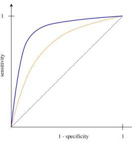
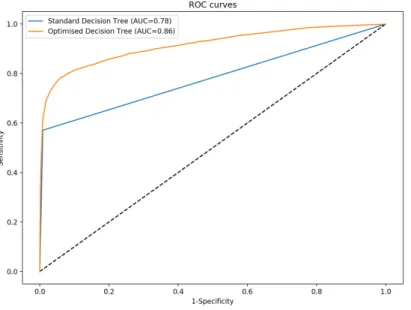
Probably the easiest way to evaluate two metrics at the same time is to plot them against each other. This is done for the sensitivity, also called true positive rate, and false positive rate which

is 1−specificity. A general plot can be seen in Figure 2.

The graph is called Receiver Operating Characteristic curve, or shortROC curve. To draw the

graph the false positive rate and true positive rate are evaluated at different thresholds. The dashed diagonal line represents the “worst” case, i.e. a model with the predictive power as good as random. The closer the ROC curve is to the dashed line, the worse is the performance of the model. Ideally the ROC curve should be close to the top left corner of the figure which represents the perfect case without any misclassifications. This means that the classifier corresponding to the blue curve is more accurate than the orange classifier. ROC analysis is useful for two main reasons. First, it depicts the trade-off between sensitivity and specificity, i.e. as sensitivity increases, specificity decreases and vice versa. And second, the area under the ROC curve, also cleverly abbreviated as

AU C (area under the curve), gives a single measure for the accuracy of the model that accounts for

(18)

Figure 2: ROC curve for two classifiers

of the model, i.e. the percentage of randomly drawn observations that are correctly predicted by the model. [10]

Additionally to specificity and sensitivity there is another measure called precision which is

defined as T P

T P+F P. The precision is thus the proportion of customers that are actually churning

and predicted as such to all predicted churners. This metric is quite similar to the sensitivity, but with the difference that instead of evaluating the proportion of correct predictions to the actual amount, the number of correct predictions versus the whole predicted amount is determined. This adds another metric by which model accuracy can be determined and again, life would be easier with just one metric. But instead of calculating the area under some curve, in this case the harmonic

mean of sensitivity and precision is calculated. This new metric is called theF1-score. In particular,

F1:= 2

S·P S+P

if sensitivity is denoted by S and precision by P. [3]

Unfortunately there is no good way to further combineAU CandF1, because they represent two

quantities that are too different. The AU C-score represents the ability of the model to correctly

predict any observation and theF1-score focuses on the ratio of correctly rejected null hypothesis,

in the churn problem that is the correctly predicted churners. Due to this difference one score might be preferred over the other in some cases. For example as previously mentioned the type-I errors

are of more interest in the churn problem, which is why the F1-score might deserve the greater

focus. However, the AU C-score is not forgotten. For the evaluation of the churn model all three

introduced measures, confusion matrix, F1 and AU C, are used in this thesis.

In this chapter the mathematical backbone of the churn model has been established. In the following text the focus lies on discussing the details of the model formulation.

(19)

3 Tree Based Methods

Step 4 of the modelling process regards the solution of the mathematical problem which is discussed in this chapter. Tree based statistical learning methods have been chosen to find a numerical

approximation of the real relationship between X and Y. This section introduces the ideas and

theory of tree based methods.

The idea can be described quite simply. Namely, the input set X is partitioned and a simple

model such as a constant is used as a prediction in each partition. Consider the following example.

Given a random vector X = [X1, X2] taking values inX ⊂IR2≥0. X can be partitioned into

M = 5 regions R1, . . . , R5 which can be seen in Figure 3a. This partitioning is equivalent to the

Decision Tree seen on the right hand side in 3b. The first split decision X1 ≤s1,1 builds the root

node. If the condition is fulfilled, the left branch is followed, otherwise the next node is formed on

the right branch. The last nodes Rm are called terminal nodes or to follow the tree analogy leaf

nodes and represent the partitions ofX.

(a) The partitioning (b) Corresponding Decision Tree

Figure 3: Partitioning of X into 5 regions

Given such partition, how does the prediction look? It remains to find a classifier f ∈F for a

given set of classifiersF ⊂F_all. A simple model for each regionRm is for example some constant

cm. That is, for each observationx0 that falls into a regionm, a constantcm particular tomserves

as prediction fory0. For anyX this means

Y =f(X) =

5

X

m=1

cmI{X ∈Rm} (2)

whereI is the indicator function,

I =

(

1 , X∈Rm

0 otherwise

In case of a classification problem,cm represents one of the possible labels inY. [11, p. 305f]

There are some questions that arise from this example and it is the task of the following sections to answer these. In particular those questions are

(20)

1. How to determine cm?

2. Which partitioning, i.e. which split conditions to choose? 3. When to stop growing the tree?

3.1 Decision Trees

The process of growing a Decision Tree is calledrecursive binary splitting. Recursive, because each

node can be further split and binary, because the splitting condition requires a binary evaluation, i.e. it is either true (to the left) or false (to the right).

To answer the first of the previously posted questions, how to determine cm in equation (2).

That is, which constant shall serve as the prediction? For a classification problem this has a straight

answer: typically themajority label k(m) of a leaf nodemis used as the prediction. Let theK+ 1

labels be denoted by k= 0, . . . , K, i.e. Y ={0, . . . , K}. Then

cm=k(m) := argmax

k

pmk (3)

wherepmk is the proportion of class k observations in m. Set Nm to be the number of samples in

m, then pmk:= 1 Nm X xi∈Rm I{yi =k} (4)

Choosing the majority label as prediction intuitively seems to be the right choice. In section 3.1.1 an argument that supports this idea is given. For regression settings the average value of all

observations inRm suffices as the predictioncm. [11, p. 307ff] This will, however, not be discussed

in further detail here.

Answering question 2 requires a definition for the best possible split. Giving such definition on the other hand requires defining some measure of the goodness of the split. This is done indirectly by inspecting the resulting nodes that can come from a split. Namely, it is of interest how “pure” the nodes are. Purity here means how homogeneous the labels in a node are. If there is a lot of

data points with the same label, then the node is rather pure, i.e. the node impurity is low. The

latter can be evaluated in three different ways. [11, p. 309] (i) Misclassification error rate,

N IM C(m) := 1

Nm X

i∈Rm

I{yi 6=k(m)}= 1−pmk(m)

Note here that though the terminology is misleading, the misclassification error rate as a node impurity measure does not correspond to the previously mentioned misclassification error as

a loss functionL(Y, f(X)). Since the loss function evaluates a wrong prediction and the node

impurity evaluates the training data, they do not substitute each other. (ii) Gini-index, N IG(m) := K X k=0 pmk(1−pmk)

(21)

(iii) Cross-entropyordeviance, N ID(m) :=− K X k=0 pmklogpmk

For a binary classification problem, i.e. k= 0 or k = 1, those measures of node impurity can

be simplified the following way. For the sake of notation setp=pm1. Thenpm0= 1−p.

(i) N IM C(m) = 1−max(p,1−p)

(ii) N IG(m) =p(1−p) +pm0(1−pm0)

=p(1−p) + (1−p)(1−1 +p)

= 2p(1−p)

(iii) N ID(m) =−(plogp+pm0logpm0)

=−plogp+ (p−1) log(1−p)

With a measure for the goodness of split, it is now possible to define the best possible split.

Given a node impurity measure N I(m) the best binary split is such that the resulting nodes R1

and R2 are purest, i.e. N I(1) and N I(2) are minimised. Finding the best partition then breaks

down to evaluating all possible splits. This is discussed in the following.

3.1.1 Growing a Classification Tree

Suppose a training data set (x1, y1), . . . ,(xN, yN)∈X ×Y withxi = (xi1, . . . , xip) fori= 1, . . . , N

is given. The observation yi takes values in Y ={0, . . . , K} which are the labels. It is the goal to

find a partition ofX intoM regions R1, . . . , RM and for each region to predict an observationy0

by f(x0) = M X m=1 cmI{x0 ∈Rm} (5)

To find the best partition, the node impurity needs to be minimised for each split. Unfortunately,

it is computationally not feasible to consider all possible splits. Instead a greedy approach is used

which means that only the best split at each step (which builds the node) is considered instead of considering all the following splits as well. [6, p. 306]

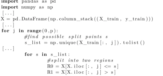
Consider a splitting variable Xj and split points. For simplicity of notation the split point sj

is just be denoted by s. The two resulting regions after the split are denoted by

R1(j, s) ={X|Xj ≤s} and R2(j, s) ={X|Xj > s}

Here the misclassification error N IM C is used. It is possible to use the other two node impurity

measures in equivalent manner. According to the definition of the best split from before, the best

j and sare then the ones that solve the following expression

min j,s min_c 1 N IM C(1) + min_c 2 N IM C(2)

(22)

By the definition of misclassification error this can be expanded to min j,s min_c 1 1−p₁_k₍₁₎+ min c2 1−p₂_k₍₂₎ = min j,s  min c1  1− 1 N1 X xi∈R1(j,s) I{yi =c1}  + min c2  1− 1 N2 X xi∈R2(j,s) I{yi=c2}     (6)

The c1 and c2 that minimise the inner expressions are the majority labels in each region given

by definition (3). With this specification it becomes feasible to iterate over all pairs (j, s) to find

the one that minimises (6). This process is then repeated for all following splits to grow a full classification tree. [11, p. 307ff]

Now that question 2 is answered, it remains to answer question 3. How large should a tree be? Tree size can be seen as the tuning parameter that determines the complexity of the model and should ideally be chosen based on the available data. Tree size is measured by the number of leaf nodes of the fully grown tree. [11, p. 308] In Section 1.3.2 model complexity is introduced by giving the example of fitting an interpolation polynomial to a set of data points. Via the degree of the polynomial the quality of fit can be regulated and that is similar to Decision Trees where

the tree size serves as the tuning parameter. If the tree grows too large the model is overfitted.

That is, it will perform well on the training data, but worse on a previously unseen observation. Consequently if the model is underfitted, i.e. the tree is too small, there is a great chance that important patterns in the data are not detected, which as well results in worse performance. This relates to the Bias-variance trade-off previously mentioned. An overfitted model usually has low bias, but high variance and vice versa for an underfitted model.

There are different methods to influence the size and therefore to control for over- or underfitting. A simple one is to select less features for the dataset and thereby to reduce the amount of possible splits. How to select the right features is discussed in a later chapter.

Another possibility is to stop growing trees at some certain fixed threshold, e.g. when there is a maximum of 5 observations in each terminal node or when the decrease in node impurity for each split is too small. There is problems with this though. First, a split that only decreases the node impurity by a little bit could possibly lead to a more valuable split later on. So a split that decreases the node impurity a lot might not happen, if the previous split was not performed. It is possible to use such threshold, but not optimal. [11, p. 308] Second, to find the optimal number of samples that each region of the partition should have it is necessary to iterate over each number. That includes growing a tree for each different setting and that easily becomes computationally heavy.

Also, typically not only one of these so calledhyper parameters needs to be optimised, but several,

which means optimising over a parameter matrix. Even though this method is computationally

heavy, it can be implemented and is then called agrid search.

An alternative is to grow a very large tree T0 and prune it back to obtain a smaller subtree,

i.e. collapse branches of T0 to “group” regions into one big one. The subtree with the lowest node

impurity in each leaf is then chosen as the best classifier. But again, it is not viable to consider

all possible subtrees, so a selective algorithm is necessary. This algorithm is calledcost complexity

pruning orweakest link pruning. [11, p. 308]

Due to the lack of this functionality in Python, tree pruning is not used here and instead a variation of the grid search is performed which is discussed later.

(23)

3.2 Method Improvements

As stated in chapter 2.3, it is the problem of binary classification to find an optimal classifier, i.e. a classifier whose expected prediction error is as close as possible to the expected prediction error of the Bayes classifier. It is also established that the difference in expected prediction errors depends on the bias and variance of the classifier and that it is therefore the goal to minimise both. By their nature, tree based methods have low bias. The bias could even vanish completely, if the tree is grown large enough. However, they tend to be of high variance. [11, p. 587f] The following sections shall discuss methods to improve predictions by reducing the variance of the classifier.

3.2.1 Bagging

Consider i.i.d. random variables X1, . . . , XN with varianceσ2. The variance of their mean is then

given by Varh¯ Xi= Var " 1 N N X i=1 Xi # = 1 N2Var "_N X i=1 Xi #

Since the random variables are i.i.d.,

Varh¯ Xi= 1 N2 "_N X i=1 VarXi # = 1 N2N σ 2 ₌ σ2 N

Hence, averaging of i.i.d. random variables reduced variance, i.e. Var ¯X <VarXi ∀i.

This idea can be applied to Decision Trees as well. Instead of just growing one tree, several trees

are grown and their predictions are averaged to obtain one bagged classifier. However, it might not

be possible to gather sufficient amounts of data sets from the prototype to grow Decision Trees on each. Instead it is possible to draw distinct sets from the original data set by repeatedly sampling

observations. The sampling is performed with replacement, i.e. the same observation (xi, yi) can

occur multiple times in each sampled data set. This sampling is calledbootstrap. [6, p. 189]

Consider a training data set T = {(x1, y1), . . . ,(xN, yN)} and draw B bootstrap samples Tb

from it withb= 1, . . . , B. For each Tb a Decision Tree is grown following the previously described

method so that a classifierfb is obtained. The bagging estimate fbag is then given by

fbag(x) = 1 B B X b=1 fb(x)

For regression trees the predictionfbag(x) is quite straight forward, i.e. it is simply the average of

all bootstrap predictions. For classification trees however, the average of the majority label does not exist. Iff :X →Y withY ={0, . . . , K}, then instead consider alabel indicatorl(x) = [l0, . . . , lK]

where li =I{f(x) =i}. If f(x) =k, then the label indicator has a one in the kth position and K

zeros otherwise so that the following holds

f(x) = argmax

k

l(x)

This idea is transferred to the bootstrap samplesTb. On thebth sample the label indicator is given

(24)

indicator, i.e. lbag(x) = " 1 B B X b=1 I{fb(x) = 0}, . . . , 1 B B X b=1 I{fb(x) =K} #

Which finally leads to an expression for the bagged classifier,

fbag(x) = argmax k " 1 B B X b=1 I{fb(x) = 0}, . . . , 1 B B X b=1 I{fb(x) =K} #! (7)

This method is described in [11, p. 282f] and the idea is that the variance offbag is lower than the

variance of fb based on the argument in the beginning of this section. However, one big problem

is that the Decision Trees grown on each sample of the training data are not independent. [11, p. 286] There is several methods to reduce the correlation between the trees, one of which is described in the next chapter.

3.2.2 Random Forest

The name “Random Forest” is not just an apt continuation of the tree-analogy of these statistical learning methods, but it also indicates the essential improvement that comes along with it. Namely, the previously mentioned de-correlation of multiple trees. A Random Forest extends the idea of

Bagging by building a set of de-correlated trees on random samples of a training data set T to

further reduce the variance of the classifier.

In the previous section it is mentioned that the mean of random variables has lower variance than the variance of each random variable. However, it was assumed that these random variables are independent which is not the case when growing Decision Trees on random samples of the same

T. Given random variables X1, . . . , XN that are identically distributed with variance σ2, but not

independent, i.e. with pairwise correlation coefficient ρ, then

Var ¯X = Var " 1 N N X i=1 Xi # =ρσ2+1−ρ N σ 2

AsN → ∞, Var ¯X →ρσ2. So the possible reduction in variance depends on the magnitude of the

correlation coefficient, which is why it is the goal here to reduce the correlation between the trees. [11, p. 588]

The method of Random Forests is similar to Bagging. Several Decision Trees are grown on

random samples of T, but in the tree growing process for each split only m ≤ p of the input

variables X1, . . . , Xp are selected as possible split candidates. The intuition is that by reducing

m, the correlation between the trees is decreased as well. [11, p. 589] For classification problems

typicallym=√

pis selected. [11, p. 592] After growing several trees that are less correlated, the

prediction of each is averaged as previously described in Section 3.2.1.

There exist other improvement possibilities of Decision Trees besides Bagging and Random Forest. In light of the scope of this thesis, other improvement methods are not discussed however. Instead the next section focuses on an evaluation of tree based methods.

3.3 Considerations

Categorical features. The problem with categorical features that have q different values

(25)

easily leads to too excessive computations. [11, p. 310] A solution to this problem is to encode

those categorical features into dummy variables by using a similar label indicator as in Section

3.2.1. For example consider a feature X1 that describes an animal type. Suppose there are N = 4

observations, X1 = [“cat”,“dog”,“cat”,“mouse”] with q = 3 different labels. In that case the

computational aspect is of course not that heavy, but examples tend to be simple in order to easily make a point. Now for each label a new “indicator feature” (the dummy variable) is introduced to the data set. This feature takes the value 1 for each observation that carries the corresponding

label. The encoded X1 then looks the following way,

X1encoded=      1 0 0 0 1 0 1 0 0 0 0 1     

The first column (feature) indicates when the animal is a cat, the second if it is a dog and the last if it is a mouse. When the Decision Tree is grown it is not necessary to find possible groupings as each new feature is already binary.

Reason for binary splits. Considering the problem with categorical features, why not allow

for multiway splits instead of only binary splits in the tree growing process? The issue with multiway splits is that they segment the data too quickly. As a result the following split might only have insufficient data available which likely leads to poor performance of the model. Additionally, multiway splits can be achieved by several binary splits in a row. Hence, there is no negative impact of only allowing for binary splits. [11, p. 311]

Imbalanced dataset. It is very common especially for binary classification problems that the

target labels in the dataset are imbalanced, e.g. in the customer data set of One.com there is much more customers that stay than those that leave. This causes a problem when the model is trained, as the class “stay” might be favoured over the class “churn”. To balance the data set it is possible todown- orup-sample it. In the former case observations of the majority class are excluded until

both classes have the same amount of observations and in the latter case, the observations of the minority class are duplicated. These methods have huge drawbacks however, since in the the first case the size of the dataset is decreased and in the latter case patterns might be introduced that

do not exist. A better method to balance the dataset is to introduceclass weights. In particular,

for each classk the weightwk is given by

wk= 1 N N X i=1 I{yi=k} (8)

where N is the number of observations (xi, yi). In the tree growing process the node impurity

measure is then evaluated by the weighted class proportions,

pwmk =

pmkwk PK

k=0pmkwk