NGUYEN, T.T., PHAM,
N.
V., DANG, M.
T.
, LUONG,
A.
V., MCCALL, J. and LIEW, A. W.-C. [2020]. Multi-layer
heterogeneous ensemble with classifier and feature selection. To presented at
2020 Genetic and evolutionary
computation conference (GECCO 2020)
, 8-12 July 2020, Cancun, Mexico. New York: ACM [online], (accepted).
Available from:
https://doi.org/10.1145/3377930.3389832
Multi-layer heterogeneous ensemble with
classifier and feature selection.
NGUYEN, T.T., PHAM,
N.
V., DANG,
M.
T., LUONG,
A.
V., MCCALL, J.
and LIEW, A. W.-C.
2020
This document was downloaded from
https://openair.rgu.ac.uk
© ACM 2020. This is the author's version of the work. It is posted here for your personal use. Not for
redistribution. The definitive Version of Record was published in 2020 Genetic and evolutionary computation
conference (GECCO 2020),
https://doi.org/10.1145/3377930.3389832
Feature Selection
Tien Thanh Nguyen
School of Computing Science and Digital Media, Robert Gordon
University Aberdeen, UK
Nang Van Pham
School of Electrical Engineering, Hanoi University of Science and
Technology Vietnam
Manh Truong Dang
School of Computing Science and Digital Media, Robert Gordon
University Aberdeen, UK
Anh Vu Luong
School of Information and Communication Technology, Griffith
University Australia
John McCall
School of Computing Science and Digital Media, Robert Gordon
University Aberdeen, UK
Alan Wee Chung Liew
School of Information and Communication Technology, Griffith
University Australia
ABSTRACT
Deep Neural Networks have achieved many successes when apply-ing to visual, text, and speech information in various domains. The crucial reasons behind these successes are the multi-layer archi-tecture and the in-model feature transformation of deep learning models. These design principles have inspired other sub-fields of machine learning including ensemble learning. In recent years, there are some deep homogenous ensemble models introduced with a large number of classifiers in each layer. These models, thus, require a costly computational classification. Moreover, the exist-ing deep ensemble models use all classifiers includexist-ing unnecessary ones which can reduce the predictive accuracy of the ensemble. In this study, we propose a multi-layer ensemble learning framework called MUlti-Layer heterogeneous Ensemble System (MULES) to solve the classification problem. The proposed system works with a small number of heterogeneous classifiers to obtain ensemble diver-sity, therefore being efficiency in resource usage. We also propose an Evolutionary Algorithm-based selection method to select the subset of suitable classifiers and features at each layer to enhance the predictive performance of MULES. The selection method uses NSGA-II algorithm to optimize two objectives concerning classifi-cation accuracy and ensemble diversity. Experiments on 33 datasets confirm that MULES is better than a number of well-known bench-mark algorithms.
CCS CONCEPTS
•Computing methodologies→Ensemble methods; • Math-ematics of computing→ Evolutionary Algorithms;
Permissiontomakedigitalorhardcopiesofallorpartofthisworkforpersonalor classroomuseisgrantedwithoutfeeprovidedthatcopiesarenotmadeordistributed forprofitorcommercialadvantageandthatcopiesbearthisnoticeandthefullcitation onthefirstpage.CopyrightsforcomponentsofthisworkownedbyothersthanACM mustbehonored.Abstractingwithcreditispermitted.Tocopyotherwise,orrepublish, topostonserversortoredistributetolists,requirespriorspecificpermissionand/ora [email protected].
GECCO’20,July8–12,2020,Cancún,Mexico
©2020AssociationforComputingMachinery.
KEYWORDS
Ensemblemethod,deeplearning,multipleclassifiers,ensembleof classifiers,featureselection,classifierselection
1
INTRODUCTION
Inrecentyears“deeplearning”hasbecomeoneofthemostpopular termsintheresearchcommunity.DeepNeuralNetworks(DNNs) haveshownoutstandingachievementsinmanysupervised learn-ingtasksforvisual,text,andspeechinformation[13].Incomputer vision,forinstance,ConvolutionalNeuralNetwork(CNN),aDNN, significantlyoutperformstraditionalmachinelearningalgorithms onthelarge-scaleImageNetclassificationtask[11].ZhouandFeng summarizedthreecrucialreasonsforthesuccessofDNNs, includ-inglayer-by-layerprocessing,in-modelfeaturetransformation,and sufficientmodelcomplexity[30].Fromthetrainingdata,DNNs gen-eratesthenewtraininginputateachlayerinwhichthenewtraining featuresreflectthedifferenthigh-levelabstractrepresentationsof theoriginaldata.Thismulti-layerdesignbringsoutdifferent as-pectsoftheoriginaldataincomparisontotheflatnetworksi.e. single-hiddenlayernetworksortraditionalmachinelearning mod-elswhichonlywork ontheoriginaldata.Moreover,DNNsare designedwithmanyhyper-parametersinmanylayers,resultingin highmodelcomplexity.Suchhighcomplexityisneededtoexplore thelargetrainingdata.
DNNsarebuiltbasedonneuralnetworksbyusing backpropa-gationtechniquetotrainmulti-layerwithdifferentiablenonlinear modules.Recently,someeffortsarebeingdonetoextenddeep learn-ingmodelswithmanylayersofensembleofclassifiers[3,21,24,30]. An ensemble is acollection of classifiers whoseprediction are combinedsoastoachievebetterperformancethanitsconstituent members.Thekeysuccessofensemblelearningresultsfromthe diverseexplorationoftheoriginaldatausingdifferenthypothesis i.e.classifiers.Byconstructingdeepensemblemodels,weexpectto
GECCO ’20, July 8–12, 2020, Cancún, Mexico T.T. Nguyen et al.
benefit from both the deep learning and ensemble learning mech-anisms. Although these deep ensemble models achieve superior classification performance on many datasets, the existing ensemble requires a large number of classifiers, resulting in huge memory usage and expensive computation. Moreover, these deep ensemble models do not perform classifier selection for each layer. In fact, the presence of some poor classifiers in each layer could degrade the system performance. We addressed these limitations by designing a multi-layer ensemble model with ensemble selection.
This paper aims to design an effective ensemble-based supervised learning system for classification inspired by the representation learning using layer-by-layer processing of DNNs. To achieve this goal, the objectives below have been specified:
•Design a novel ensemble model involving a multi-layer archi-tecture with diverse classifiers in each layer (called MULES). By combining the advantages of ensemble learning and deep learning, the proposed system is expected to perform well in many classification tasks.
•Investigate an approach to simultaneously select classifiers and the features in each layer. The proposed approach thus can overcome the limitation of existing deep ensemble mod-els by selecting only the subset of suitable classifiers and features for each layer.
•Propose fitness measures for MULES by considering not only classification accuracy but also the ensemble diversity generated by classifiers in each layer.
•Compare the performance of MULES to several existing en-semble methods and deep enen-semble models.
In Section 2, we briefly introduce ensemble learning for classifica-tion and some recent developments in Evoluclassifica-tionary Algorithms for ensemble systems. In Section 3, we give a detail description of the general architecture for the MULES. Experimental studies on a number of datasets are provided in Section 4, followed by conclusions in Section 5.
2
BACKGROUND AND RELATED WORK
2.1
Ensemble Learning
Ensemble learning explores the original data by using different hypothesis, i.e. classifiers. There are two strategies to generate the set of classifiers: heterogeneity or homogeneity [2, 4, 19]. In homo-geneous ensemble, many classifiers are obtained by training one learning algorithm on many different training sets obtained from the original one. Homogeneous ensemble uses many classifiers to ensure that the classification error converges to its asymptotic value. This thus requires huge memory storage for classifiers and high computational budgets for classification. Among many homo-geneous ensemble frameworks, Random Forest and XgBoost are the top-performance methods [4, 8]. The heterogeneous ensemble, in contrast, uses a small number of different learning algorithms on the training data to generate diverse classifiers. The research on hetero-geneous ensemble focuses on designing combining algorithms that effectively combine the predictions of the classifiers. Some examples of combining algorithms are Bayesian-based method with Mixture of Gaussians [16] and Information Granularity-based method [19]. Ensemble methods based on a multi-layer architecture is nowa-days becoming a popular trend in ensemble system design. Such
systems involve more than one layer of ensembles. Some examples of two layers of ensembles are two-layer heterogeneous ensemble [17], and a two-layer ensemble of Random Subspace and Bagging [29]. Viola and John [25] proposed a cascade model as a sequence of binary classifiers. If one classifier outputs positive value, the data is transmitted to the next classifier. A deep ensemble learning model with more than two layers called gcForest was introduced by Zhou and Feng [30] with four random forests in each layer. Utkin et al. [24] optimized gcForest by considering the weights of the trees in the same forest when averaging their predictions. These weights are found by minimizing a loss function on the training data based on the Euclidean distance between the weighted average vector and the crisp distribution vector based on the class labels of the training instances. Qi et al. [21] introduced a deep model with ensemble of SVM classifiers in each layer. The parameters of the models including the kernel functions of SVM classifiers, the number of classifiers, and the weights of features are found by using AdaBoost. In deep ensemble model in [3], the training input forithlayer is formed by concatenating the original training data and all predictions of classifiers from the 1thlayer to the(i−1)th
layer. The optimal hyper-parameters of the proposed model, includ-ing the number of classifiers in each layer, the number of layers, and the parameters for classifiers in each layer, are found by an Evolutionary Algorithm.
2.2
Selection Problem with Evolutionary
Algorithms
In the past years, many applications of Evolutionary Algorithm (EA) have been proposed to select the optimal subset of classifiers or features to improve the ensemble performance. Nguyen et al. [15] proposed the encoding of both the classifiers and six combining methods in a chromosome. The final optimal set of combining methods is combined once again using the OWA operator. Chen et al. [5] used Ant Colony Optimization (ACO) to find the optimal set of classifiers in the ensemble system. A combining algorithm is chosen from a given set of algorithms by using the uniform distribution. Wang et al. [26] used NSGA-II [6] to search for the optimal set of classifiers generated by training a regression tree on 100 new training sets. The new training data was obtained by applying the random subspace and bootstrap resampling techniques on the original training set.
EA is also widely applied to feature selection which aims to re-move redundant and irrelevant attributes to improve predictive per-formance and efficiency [28]. In ensemble learning, some EA-based feature selection methods have been proposed to select features for classifiers or to select predictions of classifiers for the combining algorithms. Kim and Cho [9] encoded the feature selection methods that will be used for each learning algorithm to learn the classi-fiers. The optimal solution is then obtained by using GA. In their extended version, the chromosomes in GA encodes the weight for each feature-classifier pair for the weighted sum combining rule. Ba-causkiene et al. [1] built the homogeneous ensemble system of SVM classifiers in which the parameters of each classifier i.e. the regular-ization constant and the kernel width and the features used by each classifier are encoded via the binary encoding scheme. Nguyen et al. [18] used ACO to simultaneously select the optimum from the
predictions of classifiers and the set of combining algorithms to improve ensemble performance.
Recently, some Evolutionary Algorithms-based approaches have been proposed for DNNs optimization in terms of their topology and hyper-parameters [14]. In [27], Genetic Algorithm was used to optimize the network structures of CNNs. The CNN network was organized in several states including ordered nodes. A binary encoding scheme was used in each stage to encode the connec-tions between the nodes insides. In [23], the three different building blocks: the convolutional layer, the pooling layer, and the fully connected layers in a CNN were encoded in one chromosome for evolution. The individuals are organized in variable-length encod-ing so as to reach the optimal depth of architecture. In [10], the hyper-parameters of DenseNet, a CNN, including the number of blocks, the number of layers in each block, and the growth rate was optimized by considering two objectives, namely computation accuracy and computational cost. The taxonomy of Evolutionary Algorithms to optimize DNNs can be found in [14].
3
PROPOSED SYSTEM
3.1
Deep Heterogeneous Ensemble System
LetD={(xn,yˆn)},|D |=Nbe the training data, wherexn∈ RDis theD-feature vector of the training instance, ˆyn ∈ Y={ym},
|Y | =Mbe its corresponding label that belongs to the label set withMlabels,K={Kk}be the set of learning algorithms|K |=K. In supervised learning (i.e. classification or regression), we aim to learn a hypothesish(i.e., classifier) for the unknown relationshipд:
xn→yˆnand use this hypothesis to assign a label for each unlabeled instance. By using an ensemble system, we train an ensemble of classifiers (EoC) onDto obtain several different hypotheses{hei}for
д. These hypotheses are then combined by a combining algorithm
C:eh=C{hei}for final decision making.
In this study, we propose MULES to solve the classification prob-lems. The proposed system has multiple layers including different classifiers in each layer. The classifiers in the first layer train on the original training data and generate the new input training data for the second layer. The classifiers in the next layer train on the new training data generated by the preceding layer and generate the new training data for the subsequent layer. A layer thus can be viewed as the feature generator which generates features for the next layer. The combining algorithm then trains on the predictions of the classifiers in the last layer for collaborated prediction. In fact, this model is based on the idea of DNNs in which the data is passed through several layers in the learning system. However, it is different from DNNs since the information in the MULES is processed under the feed-forward mechanism in which the infor-mation is only passed from one layer to the next layer and does not involve back-propagation like in neural network methods. More-over, several different learning algorithms will be used in each layer, whereas DNNs only work with layers of neurons. An illustration of MULES with a 3 layer-architecture and several different classifiers in each layer is shown in Figure 1. The outputs of the Decision Tree, Naïve Bayes, and Random Forest classifier in the first layer are combined with the original training data to generate the input for the second layer. A similar scheme is used at the second layer with two classifiers (SVM and Decision Tree) and in the third layer
with two classifiers (LDA and SVM), before the output of the third layer is combined for the final prediction.
Two following questions arise from the proposed MULES:
• How to grow the deep model?
• How to combine the predictions of the last layer to obtain the final prediction?
To grow the deep model of MULES, it is needed to generate the input data for one layer. In this study, we concatenate the original training data with the predictions of classifiers of theithlayer to form the new input data for the(i+1)th layer. We useTi-fold cross-validation on the input data for theithlayer to generate the predictions for the training data. In cross-validation, the input for
ithlayer is divided intoTidisjoint parts in which the cardinality
of each part is nearly similar. The predictions for observation in each part will obtain by using classifiers trained on the other parts. An observation thus will be predicted one time. We obtain the prediction of thekth classifier at theith layer thatxn belongs
to the class labelymdenoted byp((ki),m)(xn). We assume that the
classifiers output the predictions in the form of probability [19]:
M
Õ
m=1 p(i)
k,m(xn)=1;k=1, ...,K;n=1, ...,N (1)
LetLi denotes the new data generated by theithlayer as the input for the(i+1)thlayer(i =1,2, . . .)andL(0)=D. In this study, we propose to generateLi by concatenating the original training data and the prediction of each classifier for each observation. The augmented features, i.e. predictions and original features is expected to improve the discriminative characteristic of the training data [30]. In detail, the predictions for the training set at theithlayer is given as aN× (MK)matrixP(i)(xn)= h p(i) 1,1(xn),p (i) 1,2(xn), ...,p (i) K,M(xn) i
while the original training data is given as aN×Dmatrix. The concatenation operator will generate a new input for the(i+1)th
layer in the form of aN× (D+MK)matrix including the original training features and predictions of all instances arranged in the order as in Eqn. (3). L(i)=hL(i)(x1)...L(i)(xN) iT (2) L(i)(xn)= h xn1, ...,xnD,p1(i,)1(xn),p1(i,)2(xn), ...,pK(i),M(xn) i (3) In ensemble systems, an algorithm is used to combine the pre-dictions of classifiers for the collaborated prediction. In this study, we used the Sum Rule method for combining [10]. Sum Rule sum-marizes the predictions of each instance with regard to each class label and assigns the instance to the class label associated with the maximum value. The combined prediction on an instancexat the
ithlayer is given by:
x∈yt if t=argmaxm=1,...,M K Õ k=1 p(i) k,m(x) (4) The classification process works in a straightforward manner where a test instancexis fed forward through the layers to finally obtain
GECCO ’20, July 8–12, 2020, Cancún, Mexico T.T. Nguyen et al.
Training data Combiner Prediction
Layer (1) Layer (2) Random Forest SVM Naïve Bayes Decision Tree Decision Tree LDA SVM Layer (3)
To keep the figure simple, we do not show the concatenation between training data and the prediction of each classifier to create the input for the next layer. Figure 1: An illustration of the proposed deep heterogeneous ensemble system.
the predictions when reaching the output layer. Once again, the pre-dictions ofKclassifiers atithlayer forx, i.e.Li(x)are concatenated with the original training data in a shape of a(D+MK)-vector (3).
The prediction vector of the last layer is fed into the combiner to generate the predicted label.
3.2
Simultaneous Classifier and Feature
Selection Approach
At each layer of MULES, the original training data is concatenated to the predictions of classifiers to generate the input for the next layer. The prediction of a classifier can be viewed as scaled data from feature domain to probability domain. The new data in the proba-bility domain may have better discriminative characteristics than the original training data in case of correct predictions where obser-vations that belong to the same class will have similar prediction results and stay close together in the probability domain. However, in cases of wrong predictions, the discriminative characteristic of data will be mitigated. Concatenating the original training data and the classifier’s predictions can therefore result in better or worse discriminative characteristics than the original training data. In this work, we develop a simultaneous classifier and feature selection method for each layer of MULES in which the system performance can be improved by either removing some inconsistent classifiers in each layer or selecting the most suitable features for each selected classifier when training on the input data.
We design a two-part encoding representation for the simultane-ous classifier and feature selection method. The first part[h(i)
k ,k=
1, ...,K]of the proposed encodingE(i)in Eqn. (5) is the encoding of theKclassifiers and the second parthfkd(i),k=1, ...,K;d=1, ...,di
i
is the encoding of the features used by each classifier. In both parts, each gene in the encoding get two binary values {0,1} showing which classifiers is absence or presence in each layer (Eqn. (6)) or
which features will be used by a classifier (Eqn. (7)).
E(i)= h(i) 1 . . .h (i) K f(i) 11,f (i) 12, . . . ,f (i) 1di f(i) 21,f (i) 22, . . . ,f (i) 2di . . . f(i) K1,f (i) K2, . . . ,f (i) Kdi (5)
wheredi is the number of training features for layeri
h(i)
k =
(
1, kthclassifier is selected at layer i
0, otherwise (6)
f(i)
kd =
(
1, dthfeature is used bykthclassifier at layer i
0, otherwise (7)
In this study, the model selection is conducted at each layer to obtain the optimal set of classifiers and their features. The purpose of classifiers in all layers except the last one is to generate the input data for the next layer. Thus, the attention on only prediction accu-racy is not enough to ensure the generation of effective input data. Here we consider bi-objective optimization for the model selection problem. The first objective is the accuracy of the classification task on the validation setV:
maxE(i) 1 |V | | V | Õ n=1 Jeh (i)( xn)=yˆnK (8)
whereeh(i)is the combining model using Sum Rule at theithlayer,
| · |denotes the cardinality of a set, andJ·Kis equal 1 if the condition
is true, otherwise equal 0.
The second objective concerns the ensemble diversity generated by classifiers in each layer. It is widely recognized that diversity is an important factor to be considered when designing an ensemble system [12, 20, 30]. Kuncheva et al. [12] studied ten pairwise and non-pairwise diversity measures and examined the relationship between accuracy and diversity. Diversity was considered when designing an evaluation measure for ensemble selection (aka en-semble pruning) [20]. In this study, we measure the diversity of
0.6 0.2 0.1 0.8 0.2 0.0 New features for !" New feature for !#
Predictions of Decision Tree Predictions of Random Forest
$" $% $& 0.1 0.0 0.2 0.2 0.2 0.3 0.6 0.3 0.1 0.0 0.5 0.3 0.2 0.0 0.7 0.1 0.1 0.1 0.9 0.1 0.0 0.0 0.3 0.2 0.3 0.2 0.7 0.3 0.0 0.0
Predictions of Naïve Bayes
$' $" $% $' $& $" $% $' $& … … … … New feature for !% ("" ("% … (%" (%% … (#" (#% … … ("* (%* (#*
Original training data
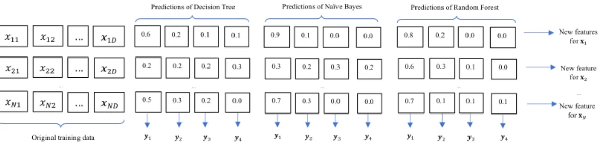
Figure 2 presents an example of the new training data generated by the first layer in Figure 1 for a four class-classification problem. Each of the three groups is the predictions of Decision Tree, Naïve Bayes, or Random Forest which show the probabilities that one instance belongs to the class labels. The new training features are concatenated with the original training data and predictions. For instances, the prediction vector (0.6, 0.2, 0.1, 0.1) in the first group shows the probabilities instance
x1belongs to class labely1,y2,y3, andy4respectively given by the Decision Tree classifier. The new training features ofx1is (x11,x12,...,x1D, 0.6, 0.2, 0.1, 0.1, 0.9,
0.1, 0.0, 0.0, 0.8, 0.2, 0.0, 0.0) will be used as the input training data for the 2ndlayer.
Figure 2: An example of the output data of the first layer in Figure 1.
classifiers in each layer by usingQ-statistic computed on the pre-dictive outcomes of two classifiers [12]:
Qij=NN00N11−N10N01
00N11+N10N01 (9)
in whichN11denotes the number of samples which are correctly
classified by both classifiers,N10denotes the number of samples
correctly classified by theithclassifier but are not correctly classi-fied by thejthclassifier.N00andN01is inversion ofN11andN10,
respectively.
TheQ-statistic diversity of theithlayer is computed by averag-ing the diversity of pairwise of selected classifiers. It is noted that the lower the value of theQ-statistic, the higher the value of the ensemble diversity. The second objective, which aims to maximize the ensemble diversity, is given by:
minE(i) 2 m(m−1) m−1 Õ i=1 m Õ j=i+1 Qij (10)
in whichmis the number of selected classifiers.
3.3
Algorithms
In the training process, MULES receives the inputs including the training dataD, the validation dataV, the learning algorithmsK
and early stopping roundsTstop. In each layer, MULES searches for the optimal subset of classifiers and features using bi-objective op-timization. Among the Evolutionary Algorithms introduced in solv-ing the multi-objective optimization problems, the non-dominated sorting genetic algorithm II (NSGA-II) is one of the most popular and effective methods [26]. NSGA-II was designed with the elitism and diversity preserving characteristics so as to find the Pareto-optimal solution (a set of non-dominated solutions) [6]. In this study, we use NSGA-II in each layer to solve the combinational optimization problem given in (8) and (10) (line 4). Since there is no clear relationship between accuracy and diversity of an ensemble [12], the use of NSGA-II makes these objectives to be considered separately, thus maintaining the richness of both criteria in the evolution process. The final result is still the prediction accuracy
as it is the main objective of interests [22, 26]. Therefore, we sim-ply choose the chromosome with the best accuracy from the last generation of NSGA-II as the final selected individual.
Based on the encoding of the selected individual, we get the set of selected classifiersH(i)and their associated featuresF(i). The selected algorithmsK(i)andF(i)is then used onL(i−1)with the Cross-Validation procedure to generate the predictions for the training instances at theithlayer i.e. aN× (MK)matrixP(i). In line 8,P(i)is concatenated with the original training dataL(0)to form the input training dataL(i)for the(i+1)thlayer.
In this study, we evaluate the predictive performance of MULES onV on each layer to automatically determine the number of layers. In line 9, we used the selectedH(i)and the selected features for each classifierF(i)onVi−1to obtain the predictionsPV(i)
i for
instances in the validation set at theithlayer. As mentioned in (4), we apply Sum Rule onPV(i)
i to obtain the predicted class label Y
(line 10). By comparingY and the ground truth of class labels of the instances inV, we can calculate the classification error rate of the
ithlayer onV(line 11). The predictionsP(i)
V1is also concatenated
with the original validation setVto obtainV(i)for the evaluation at the(i+1)thlayer.
We use a checkpoint to save the current best result and the number of layers when MULES enhances its performance on the validation set (line 13-16). After a specific number of layers, if the classification error on the validation part does not improve, we stop growing new layers and then use the checkpoint to choose the optimal number of layers.
In the testing process, an unlabeled instance is pass through all layers in MULES until reaching the last layer. In theithlayer, by referencingF(i), we can choose the features of the test instance for each selected classifier. The predictions of the selected classifiers for the test instance are concatenated to the original features to form the new training data for the next layer. We use Sum Rule on the predictions of the selected classifiers at the last layer to assign a class label for the test instance.
GECCO ’20, July 8–12, 2020, Cancún, Mexico T.T. Nguyen et al. Algorithm:MULES Input: •Training dataD=[(xn,yˆn),n=1...N] •Validation dataV=[(xi,yˆi),i=1...|V |] •K learning algorithmK
•Early stopping roundsTstop
Output:List of selected classifiers and their associated features at layeri
1 InitizlizeL(0)=D,V0=V,i=0,best_error_model=1.0 ; 2 whileTruedo
3 i++ //Train layeri;
4 Apply NGSA-II with (8) and (10) to obtain optimal
encodingEfor layer (i) ;
5 Get the set of selected classifierH(i)and their
associated featuresF(i)from E ;
6 Get the selected algorithmK(i);
7 P(i)=Cross_V alidation(K(i),F(i),L(i−1)); 8 L(i)=P(i)∪ L(0);
9 P(Vi)
i =predict
(H(i),F(i),V(i−1));
10 Y =Sum_Rule_predict(PV(i)
i)by (4) ;
11 error=Loss_f unction(Y,V);
12 V(i)=P(i)
Vi∪ V0;
13 iferror<best_error_modelthen
14 best_error_model=error;
15 Tlayer =i; 16 end
17 if errordoes not decrease afterTstoplayersthen
18 Break 19 end 20 end 21 Return h H(i)andF(i)i,i=1, ...,Tlayer s;
4
EXPERIMENTAL STUDIES
4.1
Configurations
MULES was constructed with five learning algorithms: K Nearest Neighbor (KNN, K was set to 5), Logistic Regression, Naïve Bayes (Bernoulli distribution was used), Random Forest (with 200 esti-mators), and Decision Tree. All these methods were implemented from the scikit-learn library with default parameters. We followed the experiments in [30] in which 80% of labeled data is used for the training part and the remainder is used for the validation part. We used the 2-fold Cross-Validation in one layer to generate the predic-tions for the training part. The layer growing process is stopped if the classification error rate on the validation part does not improve after 5 layers. For NSGA-II algorithm using in each layer, the maxi-mum number of generations was set to 100 and the population size was set to 50.
We used some well-known benchmark algorithms to evaluate the performance of MULES: Random Forest (with 2000 trees), gcForest
(4 forests and 500 trees in each forest), XgBoost (with 2000 trees), and Multi-Layer Perceptron (MLP). As the performance of MLP significantly depends on the network structure, we performed grid search on different parameters and reported the best result for the comparison. For MLP, we followed the experiments in [30] in which it was constructed with different configurations: input-30-20-output, input-50-30-output, and input-70-50-output.
We used the Friedman test to test the null hypothesis that all methods perform equally on all datasets. If theP-Valueof this test is smaller than a significant threshold e.g. 0.05, we reject the null hypothesis and conduct the Nemenyi post-hoc test for pairwise comparison on all datasets [7]. The experiments were conducted on 33 datasets selected from various sources such as the UCI Machine Learning Repository and OpenML1.
4.2
Experimental Results
Comparison to baselines: The prediction error rates of MULES and five benchmark algorithms are presented in Table 1. Some observations can be made:
• Based on the Friedman test, the null hypothesis was rejected with the P-Value. The Nemenyi test shows that MULES is better than XgBoost, gcForest, and MLP.
• MULES achieves the lowest average rank among all methods (rank value 1.76). On the 33 datasets, MULES ranks first in 16 cases (48.5%) and ranks second in 13 cases (39.4%). Although MULES performs poorly on 4 datasets, i.e. it ranks fourth on the Breast-Cancer and Twonorm datasets and ranks third on the Cleveland and Spambase datasets, the prediction error rates of MULES and the first rank method are not significant differences (0.0488 vs. 0.0244 of gcForest on Breast-Cancer dataset, for example).
• Random Forest and XgBoost rank second and third with average rank value 2.59 and 3.12, respectively. Random For-est ranks first on 9 datasets while XgBoost ranks first on 4 datasets. Random Forest is better than MULES on only two datasets Hayes-Roth (0.1250 vs. 0.1667) and Wine_white (0.3014 vs. 0.3449). In contrast, MULES is better than Random Forest on 6 datasets namely Chess-krvk (about 6% better), Embryonal (more than 10% better), Hill-valley (about 30% better), Madelon (about 10% better), Tic-tac-toe and Vehicle (about 5% better).
• gcForest is worse than MULES in our experiment. One some datasets such as Chess-krvk, Electricity, Hill-valley, and Iso-let, gcForest performs poorly and by far worse than MULES. gcForest ranks first on three datasets namely Breast-Cancer, Marketing, and Cleveland, but the differences in comparison to classification results of MULES are not significant.
• MLP is the poorest method in our experiment. Although MLP was run with different configurations and we reported the best result for comparisons, its performance is by far worse than MULES. On some datasets like Ring, Satimage, and
1The experimental datasets are Biodeg, Breast-Cancer, Breast-Tissue, Chess-krvk, Cleveland, Contraceptive, Electricity, Embryonal, Hayes-roth, Hill-valley, Isolet, Let-ter, Leukemia, Madelon, Magic, Marketing, Musk1, Phoneme, Ring, Satimage, Skin-NonSkin, Spambase, Texture, Tic-tac-toe, Titanic, Twonorm, Vehicle, Vertebral, Wave-form_w_noise, Waveform_wo_noise, Wine, Wine_red, Wine_white. The detail of these datasets can be found in the Supplement Material
Table 1: Classification error rate and ranking of the benchmark algorithms and MULES
gcForest MLP Random Forest XgBoost MULES
Biodeg 0.1325 (4) 0.1073 (1) 0.1230 (2.5) 0.1546 (5) 0.1230 (2.5) Breast-Cancer 0.0244 (1) 0.0488 (4) 0.0439 (2) 0.0488 (4) 0.0488 (4) Breast-Tissue 0.3125 (3.5) 0.3750 (5) 0.2813 (1.5) 0.3125 (3.5) 0.2813 (1.5) Chess-krvk 0.1882 (3) 0.3571 (5) 0.1784 (2) 0.2526 (4) 0.1280 (1) Cleveland 0.4000 (1.5) 0.5000 (5) 0.4000 (1.5) 0.4444 (4) 0.4111 (3) Contraceptive 0.4344 (3) 0.4027 (1) 0.4525 (4) 0.4615 (5) 0.4276 (2) Electricity 0.1989 (5) 0.1950 (4) 0.0937 (3) 0.0926 (2) 0.0674 (1) Embryonal 0.5000 (3.5) 0.3889 (1.5) 0.5556 (5) 0.5000 (3.5) 0.3889 (1.5) Hayes-roth 0.1667 (2.5) 0.2292 (5) 0.1250 (1) 0.1875 (4) 0.1667 (2.5) Hill-valley 0.4148 (5) 0.1058 (2) 0.3407 (4) 0.3214 (3) 0.0234 (1) Isolet 0.1863 (5) 0.0504 (2) 0.0603 (4) 0.0543 (3) 0.0483 (1) Letter 0.0360 (2) 0.0658 (5) 0.0427 (4) 0.0373 (3) 0.0332 (1) Leukemia 0.0909 (4) 0.0909 (4) 0.0455 (1.5) 0.0909 (4) 0.0455 (1.5) Madelon 0.3550 (4) 0.4550 (5) 0.3300 (3) 0.3117 (2) 0.2283 (1) Magic 0.1539 (4) 0.1604 (5) 0.1193 (1) 0.1213 (3) 0.1197 (2) Marketing 0.6418 (1) 0.6597 (3) 0.6709 (4) 0.6733 (5) 0.6563 (2) Musk1 0.1538 (2.5) 0.1748 (5) 0.1538 (2.5) 0.1678 (4) 0.1329 (1) Phoneme 0.1726 (5) 0.1369 (4) 0.0943 (1) 0.1307 (3) 0.0986 (2) Ring 0.0351 (3) 0.1568 (5) 0.0410 (4) 0.0284 (1) 0.0342 (2) Satimage 0.1253 (4) 0.1636 (5) 0.0777 (3) 0.0284 (1) 0.0756 (2)
Skin-NonSkin 1.4350E-02 (5) 8.5693E-04 (4) 5.5769E-04 (3) 4.7607E-04 (2) 4.3500E-04 (1)
Spambase 0.0608 (4) 0.0644 (5) 0.0449 (1) 0.0478 (2) 0.0492 (3) Texture 0.1564 (5) 0.0067 (1) 0.0248 (4) 0.0152 (3) 0.0145 (2) Tic-tac-toe 0.1632 (5) 0.0729 (3) 0.0764 (4) 0.0000 (1) 0.0208 (2) Titanic 0.2466 (2) 0.2496 (4) 0.2496 (4) 0.2496 (4) 0.2284 (1) Twonorm 0.0306 (5) 0.0293 (3.5) 0.0243 (2) 0.0239 (1) 0.0293 (3.5) Vehicle 0.2717 (4) 0.3110 (5) 0.2362 (3) 0.2283 (2) 0.1811 (1) Vertebral 0.2043 (4.5) 0.2043 (4.5) 0.1505 (1) 0.1935 (3) 0.1720 (2) Waveform_w_noise 0.1433 (4) 0.1633 (5) 0.1333 (2) 0.1380 (3) 0.1233 (1) Waveform_wo_noise 0.1567 (3.5) 0.1567 (3.5) 0.1427 (2) 0.1713 (5) 0.1353 (1) Wine 0.0000 (2) 0.6111 (5) 0.0000 (2) 0.0556 (4) 0.0000 (2) Wine_red 0.4146 (4) 0.4354 (5) 0.3354 (2) 0.3604 (3) 0.3250 (1) Wine_white 0.4252 (4) 0.4837 (5) 0.3014 (1) 0.3490 (3) 0.3449 (2) Average Ranking 3.59 3.94 2.59 3.12 1.76
Table 2: An example of the obtained configuration for MULES on Tic-tac-toe dataset
Classifiers Features Encoding
Layer 1
Random Forest (200) 6 original features 011010111 Decision Tree 6 original features 111110100 KNN(5) 5 original features 100100111
Layer 2
Random Forest (200) 5 original features + 1 prediction 100010111 | 000100 Naïve Bayes 7 original features + 5 predictions 001111111 | 111110 KNN(5) 4 original features + 4 predictions 100101100 | 111010 Logistic Regression 6 original features + 2 predictions 011110110 | 010010
Layer 3 KNN(5) 4 original features + 8 predictions 101001100 | 10111111 Logistic Regression 3 original features + 6 predictions 011000100 | 10011111
Layer 4 KNN(5) 3 original features + 2 predictions 001001001 | 1010 Logistic Regression 3 original features + 1 prediction 100010001 | 0010
Vehicle, the classification error rates of MLP are significantly higher than those of MULES.
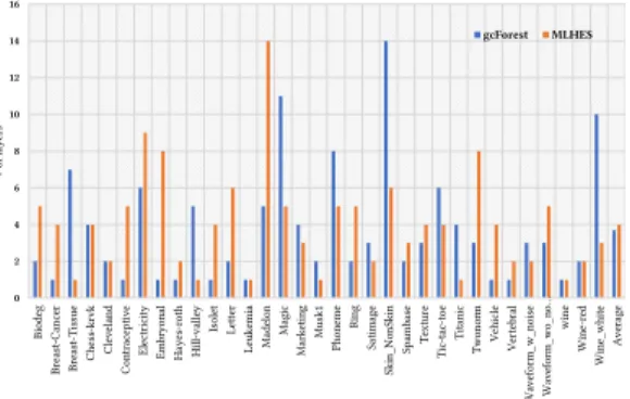
The number of layers and configuration: Figure 4 presents the comparisons between the number of layers generated by gc-Forest and MULES on the experimental datasets. Like gcgc-Forest, MULES can automatically determine the number of layers based on its prediction performance on the validation set. On average, MULES generated 4 layers of ensemble of classifiers. This means going deeply can improve the performance of the deep model on the validation data of some datasets. Moreover, MULES generated
1 2 3 4 CD MULES Random Forest XgBoost gcForest MLP
Figure 3: The Nememyi test result
more number of layers than gcForest, 4 compared to 3.7 on average. Exceptionally, both methods generate only one layer on 9 and 6 datasets. In these cases, going deeply with the new proposed input data does not bring benefits to the ensemble system.
We further analyze the benefits of the multi-layer architecture in MULES. Figure 5 shows the reductions of the prediction error rates on the test data of MULES through layers in the deep model. On Hayes-Roth dataset, for example, where MULES generates the model with 2 layers, the prediction error rate reduces from 0.1875 to 0.1667. On Tic-Tac-Toe dataset, the prediction error rate reduces from 0.1042 to 0.059 from the first layer to second layer, and con-tinue to reduce to 0.0486 at the third layer and to 0.0208 at the fourth layer. This figure demonstrates the advantages of layer-by-layer
GECCO ’20, July 8–12, 2020, Cancún, Mexico T.T. Nguyen et al. 0 2 4 6 8 10 12 14 16 B io deg B rea st -C an ce r B rea st -T is su e C hes s-kr vk C lev ela nd C on tr ac ep ti ve El ec tr ic ity Em br yo na l H ay es -r oth H ill-va lle y Is ole t Let ter Le uk emi a M ad elo n Ma gi c M ar ket in g Mu sk 1 Ph on eme Rin g Sa ti m ag e Sk in _N on Ski n Sp amb as e T ex tu re T ic -ta c-toe Ti ta ni c Tw on or m V eh ic le V er teb ra l W ave fo rm _w _n oi se W ave fo rm _w o_ no … wi ne W in e-re d Wi ne _w hi te A ve ra ge # of la yer s gcForest MLHES
Figure 4: The number of layers obtained by gcForest and MULES. 0,02 0,04 0,06 0,08 0,10 0,12
Layer 1 Layer 2 Layer 3 Layer 4 Layer 5
C la ss if ic at ion E rr or R at e
Ring Satimage Spambase Tic-tac-toe
0,12 0,14 0,16 0,18 0,20
Layer 1 Layer 2 Layer 3 Layer 4 Layer 5
C la ss if ic at ion E rr or R at e
Biodeg Chess-krvk Hayes-roth Vertebral
Figure 5: The changes of classification error rate in each layer.
processing in MULES since the classification system gets better results with deeper layer.
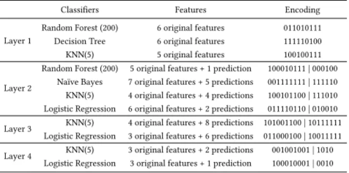
We illustrate an example of the obtained configuration for MULES on the Tic-tac-toe dataset. At each layer, MULES selected the suit-able classifiers and their features to generate the input for the next layer. In detail, on the first layer, MULES chose 3 classifiers: Ran-dom Forest, Decision Tree, and KNN. Each classifier used its own features selected from the original features. In the second layer, classifiers except Decision Tree were selected with different feature sets obtained from the original features and predictions. On the third and fourth layers, two classifiers KNN and Logistic Regression were selected with different feature sets. By selecting the suitable
classifiers in each layer and suitable features for each classifier, MULES can obtain high prediction accuracy and effectiveness in resource usage in terms of memory and computation requirements.
Classification time: Although MULES takes much higher train-ing time than gcForest, the classification time of MULES is lower than gcForest. On Tic-tac-toe dataset, for example, MULES used 3154.86 second for training process compared to only 311.78 of gcForest. Meanwhile, gcForest used 0.62 second to classify all test instances while MULES only used 0.26 second.
MULES obtains a subset of classifiers and their features in each layer. From the obtained configuration for Tic-tac-toe dataset in Table 2, after the evolution process, only 3 and 4 classifiers were kept in the first and second layer. The third and fourth layer only have 2 classifiers. Therefore, only 11 classifiers are maintained in MULES to classify instances on this dataset. That makes MULES takes less time during classification. In contrast, gcForest used 4 Random Forests involving 500 trees in each forest. MLP also takes high computation for the training process as its configuration is somehow problem-dependent that requires a procedure to search for the optimal one. It is noted that like population-based Evolution Algorithms, NSGA-II can be implemented in parallel. This can further reduce the training time of MULES.
5
CONCLUSIONS
In summary, we introduced a Multi-Layer Heterogeneous Ensem-ble System (MULES) inspired by the layer-by-layer processing of DNNs. MULES includes several layers of the ensemble of different classifiers in which the classifiers in one layer train on the new training data generated by the preceding layer. The new training data for one layer is the concatenation of the predictions of the classifiers in the preceding layer and the original training data. We train a combining algorithm on the predictions of classifiers in the last layer for the final collaborated prediction. Since the ensemble in each layer can contain the unnecessary classifiers which increase the prediction error of the ensemble, we propose an Evolutionary Algorithm-based method to select the optimal set of classifiers and their features on each layer. The optimization problem is considered under two objectives concerning the prediction error and ensemble diversity. We used NSGA-II, a popular and effective multi-objective evolutionary algorithm, to solve this optimization problem.
Experiments on 33 datasets confirm that MULES is better than MLP, Random Forest, gcForest, and XgBoost in terms of predictive performance and efficiency.
Two solutions to enhance the performance of MULES could be implemented in the future. First, in this study we concatenated the original training data and the predictions of classifiers in one layer to generate the input data for the next layer. In general, MULES can generate multiple layers and its prediction accuracy becomes better on the deeper layers. The exception occurred on 6 datasets where going deeply does not achieve any improvements for the classification process. A new input data is needed to populate the deep model in these cases. Second, we used NSGA-II to search for the set of classifiers and their features in each layers. Parallel implementation of NSGA-II can be used in MULES to reduce its training time.
REFERENCES
[1] Marija Bacauskiene, Antanas Verikas, Adas Gelzinis, and Donatas Valincius. 2009. A feature selection technique for generation of classification committees and its application to categorization of laryngeal images.Pattern Recognition42, 5 (2009), 645–654.
[2] Leo Breiman. 2001. Random forests.Machine learning45, 1 (2001), 5–32. [3] Boyuan Chen, Harvey Wu, Warren Mo, Ishanu Chattopadhyay, and Hod Lipson.
2018. Autostacker: A compositional evolutionary learning system. InProceedings of the Genetic and Evolutionary Computation Conference. 402–409.
[4] Tianqi Chen and Carlos Guestrin. 2016. Xgboost: A scalable tree boosting system. InProceedings of the 22nd acm sigkdd international conference on knowledge discovery and data mining. 785–794.
[5] Yijun Chen and Man Leung Wong. 2011. Optimizing stacking ensemble by an ant colony optimization approach. InProceedings of the 13th annual conference companion on Genetic and evolutionary computation. 7–8.
[6] Kalyanmoy Deb, Amrit Pratap, Sameer Agarwal, and TAMT Meyarivan. 2002. A fast and elitist multiobjective genetic algorithm: NSGA-II.IEEE transactions on evolutionary computation6, 2 (2002), 182–197.
[7] Janez Demšar. 2006. Statistical comparisons of classifiers over multiple data sets.
Journal of Machine learning research7, Jan (2006), 1–30.
[8] Manuel Fernández-Delgado, Eva Cernadas, Senén Barro, and Dinani Amorim. 2014. Do we need hundreds of classifiers to solve real world classification problems?The journal of machine learning research15, 1 (2014), 3133–3181. [9] Kyung-Joong Kim and Sung-Bae Cho. 2008. An evolutionary algorithm approach
to optimal ensemble classifiers for DNA microarray data analysis.IEEE Transac-tions on Evolutionary Computation12, 3 (2008), 377–388.
[10] Josef Kittler, Mohamad Hatef, Robert PW Duin, and Jiri Matas. 1998. On combin-ing classifiers.IEEE transactions on pattern analysis and machine intelligence20, 3 (1998), 226–239.
[11] Alex Krizhevsky, Ilya Sutskever, and Geoffrey E Hinton. 2012. Imagenet classifica-tion with deep convoluclassifica-tional neural networks. InAdvances in neural information processing systems. 1097–1105.
[12] Ludmila I Kuncheva and Christopher J Whitaker. 2003. Measures of diversity in classifier ensembles and their relationship with the ensemble accuracy.Machine learning51, 2 (2003), 181–207.
[13] Yann LeCun, Yoshua Bengio, and Geoffrey Hinton. 2015. Deep learning.nature
521, 7553 (2015), 436–444.
[14] Pablo Ribalta Lorenzo and Jakub Nalepa. 2018. Memetic evolution of deep neural networks. InProceedings of the Genetic and Evolutionary Computation Conference. 505–512.
[15] Tien Thanh Nguyen, Alan Wee-Chung Liew, Xuan Cuong Pham, and Mai Phuong Nguyen. 2014. Optimization of ensemble classifier system based on multiple objectives genetic algorithm. In2014 International Conference on Machine Learning and Cybernetics, Vol. 1. IEEE, 46–51.
[16] Tien Thanh Nguyen, Alan Wee-Chung Liew, Minh Toan Tran, and Mai Phuong Nguyen. 2014. Combining multi classifiers based on a genetic algorithm–a
gaussian mixture model framework. InInternational Conference on Intelligent Computing. Springer, 56–67.
[17] Tien Thanh Nguyen, Alan Wee-Chung Liew, Minh Toan Tran, Thi Thu Thuy Nguyen, and Mai Phuong Nguyen. 2014. Fusion of classifiers based on a novel 2-stage model. InInternational Conference on Machine Learning and Cybernetics. Springer, 60–68.
[18] Tien Thanh Nguyen, Anh Vu Luong, Thi Minh Van Nguyen, Trong Sy Ha, Alan Wee-Chung Liew, and John McCall. 2019. Simultaneous data and meta-classifier selection in multiple meta-classifier system. InProceedings of the Genetic and Evolutionary Computation Conference. 39–46.
[19] Tien Thanh Nguyen, Mai Phuong Nguyen, Xuan Cuong Pham, Alan Wee-Chung Liew, and Witold Pedrycz. 2018. Combining heterogeneous classifiers via granular prototypes.Applied Soft Computing73 (2018), 795–815.
[20] Ioannis Partalas, Grigorios Tsoumakas, and Ioannis Vlahavas. 2010. An ensemble uncertainty aware measure for directed hill climbing ensemble pruning.Machine Learning81, 3 (2010), 257–282.
[21] Zhiquan Qi, Bo Wang, Yingjie Tian, and Peng Zhang. 2016. When ensemble learn-ing meets deep learnlearn-ing: a new deep support vector machine for classification.
Knowledge-Based Systems107 (2016), 54–60.
[22] Jacob Schrum. 2018. Evolving indirectly encoded convolutional neural networks to play tetris with low-level features. InProceedings of the Genetic and Evolutionary Computation Conference. 205–212.
[23] Yanan Sun, Bing Xue, Mengjie Zhang, and Gary G Yen. 2019. Evolving deep convolutional neural networks for image classification.IEEE Transactions on Evolutionary Computation(2019).
[24] Lev V Utkin, Maxim S Kovalev, and Anna A Meldo. 2019. A deep forest classifier with weights of class probability distribution subsets.Knowledge-Based Systems
173 (2019), 15–27.
[25] Paul Viola and Michael Jones. 2001. Rapid object detection using a boosted cascade of simple features. InProceedings of the 2001 IEEE computer society conference on computer vision and pattern recognition. CVPR 2001, Vol. 1. IEEE, I–I. [26] Yuyan Wang, Dujuan Wang, Na Geng, Yanzhang Wang, Yunqiang Yin, and Yaochu
Jin. 2019. Stacking-based ensemble learning of decision trees for interpretable prostate cancer detection.Applied Soft Computing77 (2019), 188–204. [27] Lingxi Xie and Alan Yuille. 2017. Genetic cnn. InProceedings of the IEEE
interna-tional conference on computer vision. 1379–1388.
[28] Bing Xue, Mengjie Zhang, Will N Browne, and Xin Yao. 2015. A survey on evolutionary computation approaches to feature selection.IEEE Transactions on Evolutionary Computation20, 4 (2015), 606–626.
[29] Zhiwen Yu, Daxing Wang, Jane You, Hau-San Wong, Si Wu, Jun Zhang, and Guoqiang Han. 2016. Progressive subspace ensemble learning.Pattern Recognition
60 (2016), 692–705.
[30] Zhi-Hua Zhou and Ji Feng. 2017. Deep Forest: Towards An Alternative to Deep Neural Networks. InProceedings of the Twenty-Sixth International Joint Conference on Artificial Intelligence, IJCAI-17. 3553–3559. https://doi.org/10.24963/ijcai.2017/ 497