1 2 3 4 5 6 7 8 9 10 11 12 13 14 15 16 17 18 19 20 21 22 23 24 25 26 27 28 29 30 31 32 33 34 35 36 37 38 39 40 41 42 43 44 45 46 47 48 49 50 51 52
ClassiNet – Predicting Missing Features for Short-Text
Classification
∗ C o nsist en Complete*W ellD o cu m en ted *E asy to Re us e * * Ev alu ate d * Po P *Ar AEC P PDANUSHKA BOLLEGALA
†and VINCENT ATANASOV,
University of LiverpoolTAKANORI MAEHARA,
RIKEN Center for Advanced Intelligence ProjectKEN-ICHI KAWARABAYASHI,
National Institute of InformaticsShort and sparse texts such as tweets, search engine snippets, product reviews, chat messages are abundant on the Web. Classifying
such short-texts into a pre-defined set of categories is a common problem that arises in various contexts, such as sentiment classification,
spam detection, and information recommendation. The fundamental problem in short-text classification isfeature sparseness– the
lack of feature overlap between a trained model and a test instance to be classified. We proposeClassiNet– a network of classifiers
trained for predicting missing features in a given instance, to overcome the feature sparseness problem. Using a set of unlabeled
training instances, we first learn binary classifiers as feature predictors for predicting whether a particular feature occurs in a given
instance. Next, each feature predictor is represented as a vertexviin the ClassiNet where a one-to-one correspondence exists between
feature predictors and vertices. The weight of the directed edgeei jconnecting a vertexvito a vertexvjrepresents the conditional
probability that givenviexists in an instance,vjalso exists in the same instance.
We show that ClassiNets generalize word co-occurrence graphs by considering implicit co-occurrences between features. We
extract numerous features from the trained ClassiNet to overcome feature sparseness. In particular, for a given instancex, we find
similar features from ClassiNet that did not appear inx, and append those features in the representation ofx. Moreover, we propose
a method based on graph propagation to find features that are indirectly related to a given short-text. We evaluate ClassiNets on
several benchmark datasets for short-text classification. Our experimental results show that by using ClassiNet, we can statistically
significantly improve the accuracy in short-text classification tasks, without having to use any external resources such as thesauri for
finding related features.
CCS Concepts: •Information systems→Content analysis and feature selection;
Additional Key Words and Phrases: Classifier Networks, Feature Sparseness, Short-Texts, Text Classification
ACM Reference format:
Danushka Bollegala, Vincent Atanasov, Takanori Maehara, and Ken-ichi Kawarabayashi. 2017. ClassiNet – Predicting Missing Features
for Short-Text Classification.ACM Trans. Knowl. Discov. Data.0, 0, Article 0 ( 2017),29pages.
https://doi.org/0000001.0000001
∗
†
The corresponding author
This work is supported by the ERATO Kawarabayashi Large Graph Project from the Japan Science and Technology Agency ( JST)..
Permission to make digital or hard copies of all or part of this work for personal or classroom use is granted without fee provided that copies are not
made or distributed for profit or commercial advantage and that copies bear this notice and the full citation on the first page. Copyrights for components
of this work owned by others than ACM must be honored. Abstracting with credit is permitted. To copy otherwise, or republish, to post on servers or to
redistribute to lists, requires prior specific permission and /or a fee. Request permissions from [email protected].
© 2017 Association for Computing Machinery.
Manuscript submitted to ACM
53 54 55 56 57 58 59 60 61 62 63 64 65 66 67 68 69 70 71 72 73 74 75 76 77 78 79 80 81 82 83 84 85 86 87 88 89 90 91 92 93 94 95 96 97 98 99 100 101 102 103 104 1 INTRODUCTION
Short-texts are abundant on the Web and appear in various different formats. For example, in Twitter, users are
constrained to a 140 character upper limit when posting their tweets [Kwak et al. 2010]. Even when there are no strict
upper limits, users tend to provide brief answers in QA forums, review sites, SMS, email, and chat messages [Cong
et al. 2008;Thelwall et al. 2010]. Unlike lengthy responses that take time to both compose and to read, short responses
have gained popularity particularly in social media contexts. Considering the steady growth of mobile devices that are
physically restricted to compact keyboards, which are suboptimal for entering lengthy text inputs, it is safe to predict
that the amount of short-texts will continue to grow in the future. Considering the importance and the quantity of the
short-texts in various web-related tasks, such as text classification [dos Santos and Gatti 2014;kun Wang et al. 2012],
and event prediction [Sakaki et al. 2010], it is important to be able to accurately represent and classify short-texts.
Compared to performing text mining on longer texts [Guan et al. 2009;Su et al. 2011;Yogatama and Smith 2014], for
which dense and diverse feature representations can be created relatively easily, handling of shorter texts poses several
challenges. First, the number of features that are actually present in a short-text will be a small fraction of the set of all
features that exist in all of the train instances. Although thisfeature sparsenessis problematic even for longer texts, it is critical for shorter texts. In particular, when the diversity of the feature space increases as with longern-gram lexical features, (a) the number of occurrences of a feature in a given instance (i.e., term frequency), as well as (b) the number
of instances in which a particular feature occurs (i.e., document frequency), will be small. Therefore, it is difficult to
reliably estimate the salience of a feature in a particular class in supervised learning tasks.
Second, the shorter length means that there isless redundancyin terms of the features that exist in a short-text. Consequently, most of the related words of a particular word might be missing in a short-text. For example, consider
a review oniPhone 6that says “I liked the larger screen size of iPhone 6 compared to that of its predecessor”. Although iPhone 6 plus, a product similar toiPhone 6, has also a larger screen compared to its predecessors, this information is not included in this short review. On the other hand, we might observe such positive sentiments associated withiPhone 6 plusbut not withiPhone 6in other train instances, which will result in a high positive score foriPhone 6 plusin a classifier trained from those train reviews. Unfortunately, we will not be able to infer that this particular user would
also likely be satisfied withiPhone 6 plus, thereby not recommendingiPhone 6 plusfor this user.
To overcome the above-mentioned challenges encountered when handling short-texts, we propose afeature ex-pansionmethod analogous to the query expansion methods used in information retrieval (IR) [Salton and Buckley 1983] to improve the agreement between search queries input by the users and documents indexed by the search
engine [Carpineto and Romano 2012]. We assume short-texts are already represented using some feature vectors,
which we refer to asinstancesin this paper. Lexical features such as unigrams or bigrams of words, part-of-speech (POS) tag sequences, and dependency relations have been frequently used in prior work on text classification. Our
proposed method does not assume any particular type of features, and can be used with any discrete feature set. First,
we train binary classifiers which we callfeature predictorsfor predicting whether a particular featurevioccurs in a given instancex. For example, given the previously discussed short review, we would like to predict whether iPhone 6 plus is likely to occur in this review.
The training instances required to learn feature predictors are automatically selected from unlabeled texts. Specifically,
given a featurevi, we select texts in whichvioccurs as the positive training instances for learning a feature predictor forvi. On the other hand, negative training instances for learning the feature predictor forvi are randomly sampled from the unlabeled texts, wherevi does not occur. Using those positive and negative training instances we learn a
105 106 107 108 109 110 111 112 113 114 115 116 117 118 119 120 121 122 123 124 125 126 127 128 129 130 131 132 133 134 135 136 137 138 139 140 141 142 143 144 145 146 147 148 149 150 151 152 153 154 155 156
binary classifier to predict whethervioccurs in a given instance. Any binary classification algorithm, such as support vector machines, logistic regression, naive Bayes classifier etc. can be used for this purpose, and it is not limited to
linear classifiers. We defineClassiNetas a directed weighted graphG(V,E,W)of feature predictors, where each vertex vi ∈ Vcorresponds to a feature predictor. The directed edgeei j ∈ Efromvi tovj is assigned the weight 1≥wi j≥0, which is the conditional probability that givenviis predicted for a particular instance,vjis also predicted for the same instance.
It is noteworthy that we obtain both positive and negative instances for learning feature predictors from unlabeled
data, and do not require any labeled data for the target task. For example, consider the case that we are creating a
ClassiNet to find missing features in sentiment classification. In this case, the target task is sentiment classification.
However, we do not require any labeled data for the target task such as sentiment annotated reviews when creating
the ClassiNet that we are subsequently going to use for finding missing features. Therefore, the training of ClassiNets
can be conducted in a purely unsupervised manner, without requiring any manually labeled data for the target task.
Moreover, the decoupling of ClassiNet training from the target task enables us to use the same ClassiNet to expand
feature vectors for different target tasks. As we discuss later in Section3.4, ClassiNets can be seen as a generalized
version of the word co-occurrence graphs that have been well-studied in the NLP community [Mihalcea and Radev
2011]. However, ClassiNets consider both explicit as well as implicit co-occurrences of words in some context, whereas
word co-occurrence graphs are limited to explicit co-occurrences.
Given a ClassiNet created from unlabeled data as described above, we propose several strategies for finding related
features for a given instance that do not occur in the original instance. Specifically, we compare bothlocalfeature expansion methods that consider the nearest neighbours of a particular feature in an instance (Section4.1), as well as
globalfeature expansion methods that propagate the features that exist in an instance over the entire set of vertices in ClassiNet (Section4.2). We evaluate the performance of the proposed feature expansion methods on short-text
classification benchmark datasets. Our experimental results show that the proposed global feature expansion method
significantly outperforms several local feature expansion methods„ and several sentence-level embedding methods on
multiple benchmark datasets proposed for evaluating short-text classification methods. Considering that (a) ClassiNets
can be created using unlabeled data, (b) the same ClassiNet can be used in principle for predicting features for different
target tasks, (c) arbitrary features could be used in the feature predictors, not limited to lexical features, we believe that
ClassiNets can be applied to a broad-range of machine learning tasks, not limited to short-text classification.
Our contributions in this paper can be summarised as follows:
• We propose a method for learning a network of feature predictors that can predict missing features in feature vectors. The proposed network, which we refer to as the ClassiNet, can be learnt in an unsupervised manner,
without requiring any labeled data for the target task in which we are going to apply the ClassiNet to expand
features (Section3.2).
• We propose an efficient method to learn ClassiNets from large datasets. Specifically, we show that the edge-weights of ClassiNets can be computed efficiently using locality sensitive hashing (Section3.3).
• Having proposed ClassiNets, we describe its relationship to word co-occurrence graphs that have a long history in the NLP community. We show that ClassiNets can be considered as a generalised version of word
co-occurrence graphs (Section3.4).
• We propose several methods for finding related features for a given instance using the created ClassiNet. In particular, we consider bothlocal methods(Section4.1) that consider the nearest neighbours in ClassiNet of
157 158 159 160 161 162 163 164 165 166 167 168 169 170 171 172 173 174 175 176 177 178 179 180 181 182 183 184 185 186 187 188 189 190 191 192 193 194 195 196 197 198 199 200 201 202 203 204 205 206 207 208
the features that exist in an instance, as well asglobal methods(Section4.2) that consider all vertices in the ClassiNet.
2 RELATED WORK
Feature sparseness is a common problem that is encountered in various text mining tasks. Two main approaches for
overcoming the feature sparseness problem in short-texts can be identified in the literature: (a) embedding the train/test
instances in a dense, lower-dimensional feature space thereby reducing the number of zero-valued features in the
instances, and (b) predicting the values of the missing features. Next, we discuss prior work that belong to each of those
two approaches.
An effective technique frequently used in prior work on short-texts to overcome the feature sparseness problem is to
represent the texts in some lower-dimensional dense space, thereby reducing the feature sparseness. Several methods
have been used to obtain such lower-dimensional representations such as topic-models [kun Wang et al. 2012;Yan
et al. 2013;Yang et al. 2015], clustering [Dai et al. 2013;Rangrej et al. 2011], and dimensionality reduction [Blitzer et al.
2006;Pan et al. 2010]. Wang et al. [kun Wang et al. 2012] used latent dirichlet allocation (LDA) to identify features that
are useful for identifying a particular class. Higher weights are assigned to the identified features, thereby increasing
their contribution towards the classification decision. However, applying LDA at sentence-level is problematic because
the number of words in a sentence is much smaller than that in a document. Consequently, Yan et al. [Yan et al. 2013]
proposed the bi-term topic model that models the co-occurrence patterns between words accumulated over the entire
corpus. An alternative solution that uses an external knowledge-base in the form of a phrase list is propsed by Yang et
al. [Yang et al. 2015] to overcome the feature sparseness problem when learning topics from short-texts. The phrase list
is automatically extracted from the entire collection of short-texts in a pre-processing step.
Cluster-based methods have been proposed for representing documents to overcome the feature sparseness problem.
First, some clustering algorithm is used to cluster the documents into a group of clusters. Next, each document is
represented by the clusters to which it belongs. Dai et al. [Dai et al. 2013] used a hierarchical clustering algorithm
with purity control to generate a set of clusters, and use the similarity between a document and each of the clusters
as augmented features to enrich the document representation. Their method significantly improves the classification
accuracy for short web snippets in a support vector machine classifier. Feature mismatch is a fundamental problem in
domain adaptation, where we must learn a classifier using labeled data from a source domain and apply it to predict
labels for the test instances in a different target domain. Pan et al. [Pan et al. 2010] proposed Spectral Feature Alignment
(SFA), a method to overcome the feature mismatch problem in cross-domain sentiment classification. They created a
bi-partite graph between domain-specific and domain-independent features, and then used a spectral clustering method
to obtain a domain-independent lower-dimensional embedding.
In structural correspondence learning (SCL) [Blitzer et al. 2007,2006], a set of features that are common to both
source and the target domains, referred to aspivots, is identified using mutual information with the sentiment label. Next, linear classifiers that can predict those pivots are learnt from unlabeled reviews. The weight vectors corresponding
to the learnt linear classifiers are arranged as rows in a matrix, on which subsequently singular value decomposition is
applied to compute a lower-dimensional projection. Feature vectors representing train source reviews are projected
into this lower-dimensional space, in which a binary sentiment classifier is trained. During test time, feature vectors
representing test target reviews are also projected to the same lower-dimensional space and the trained binary classifier
is used to predict the sentiment labels. However, domain adaptation methods such as SCL and SFA require data from at
209 210 211 212 213 214 215 216 217 218 219 220 221 222 223 224 225 226 227 228 229 230 231 232 233 234 235 236 237 238 239 240 241 242 243 244 245 246 247 248 249 250 251 252 253 254 255 256 257 258 259 260
least two (source vs. target) different domains (e.g. reviews on products in different categories) to overcome the missing
feature problem, whereas in this work we assume the availability of data from one domain only.
Instead of representing documents using lexical features, which often results in high-dimensional and sparse feature
vectors, by embedding documents in low-dimensional dense spaces we can effectively overcome the feature sparseness
problem [dos Santos and Gatti 2014;Le and Mikolov 2014;Lu and Li 2013]. These methods jointly learn character-level
or word-level embeddings as well as document-level embeddings [Hill et al. 2016a;Kiros et al. 2015] such that the learnt
embeddings capture the similarity constraints satisfied by a collection of short-texts. First, each word in the vocabulary
is assigned a fixed dimensional word vector. We can initialize the word vectors randomly or using pre-trained word
representations. Next, the word vectors are updated such that we can accurately predict the co-occurrences of words in
some context, such as a window of tokens, a sentence, a paragraph, or a document. Different loss functions encoding
different co-occurrence measures have been proposed for this purpose [Mikolov et al. 2013;Pennington et al. 2014]. As
shown later in Section6.2, ClassiNets perform competitively against sentence-level embedding methods on several
short-text classification tasks.
A single word can have multiple senses. For example, the wordbankcould mean afinancial institutionor ariver bank. Therefore, it is inadequate to represent different senses of a word using a single embedding [Camacho-Collados et al.
2015;Hu et al. 2016;Iacobacci et al. 2015a;Johansson and Nieto Piña 2015;Li and Jurafsky 2015;Reisinger and Mooney
2010;Song et al. 2016]. Several solutions have been proposed in the literature to overcome this limitation and learnsense embeddings, which capture the sense related information of words. For example,Reisinger and Mooney[2010] proposed a method for learning sense-specific high dimensional distributional vector representations of words, which was later
extended byHuang et al.[2012] using global and local context to learn multiple sense embeddings for an ambiguous
word.Neelakantan et al.[2014] proposed a multi sense skip-gram (MSSG), an online cluster-based sense-specific word
representations learning method, by extending Skip-Gram with Negative Sampling (SGNG) [Mikolov et al. 2013]. Unlike
SGNG, which updates the gradient of the word vector according to the context, MSSG predicts the nearest sense first,
and then updates the gradient of the sense vector.
Aforementioned methods apply a form of word sense discrimination by clustering a word contexts, before learning
sense-specific word embeddings based on the induced clusters to learn a fixed number of sense embeddings for each
word. In contrast, a nonparametric version of MSSG (NP-MSSG) [Neelakantan et al. 2014] estimates the number of
senses per word and learn the corresponding sense embeddings. On the other hand,Iacobacci et al.[2015b] used a Word
Sense Disambiguation (WSD) tool to sense annotate a large text corpus and then used an existing prediction-based word
embeddings learning method to learn sense and word embeddings with the help of sense information obtained from the
BabelNet [Iacobacci et al. 2015b] sense inventory. Similarly,Camacho-Collados et al.[2015] used the knowledge in two
different lexical resources: WordNet [Miller 1995] and Wikipedia. They use the contextual information of a particular
concept from Wikipedia and WordNet synsets prior to learning two separate vector representations for each concept.
A single word can be related to multiple different topics, without necessarily corresponding to different senses of
the word. Revisiting our previous example, we might have a collection of documents aboutretail banks,commercial banks,investment banksandcentral banks. All these different banks are related to the financial sense of the word bank. However, in a particular task (eg. classifying documents related to the different types of financial banks), we might
require different embeddings for the different topics in which the word bank appears.Liu et al.[2015a] proposed three
methods for learningtopical word embeddings, where they first cluster words into different topics using LDA [Blei et al. 2003] and then learn word embeddings using SGNS.Liu et al.[2015b] modelled the interactions among topics,
261 262 263 264 265 266 267 268 269 270 271 272 273 274 275 276 277 278 279 280 281 282 283 284 285 286 287 288 289 290 291 292 293 294 295 296 297 298 299 300 301 302 303 304 305 306 307 308 309 310 311 312
contexts and words using a tensor and obtained topical word embeddings via tensor factorisation. Instead of clustering
words prior to embedding learning,Shi et al.[2017] proposed a method to jointly learn both words and topics, thereby
considering the correlations between multiple senses of different words that occur in different topics. TopicVec [Li et al.
2016a] learns vector representations for topics in a document by modelling the co-occurrence between a target word
and a context word considering both words’ word embeddings as well as the topic embedding of the context word.
Our proposed methods for feature expansion using ClassiNet can be seen as anexplicitfeature prediction method, whereas methods that learn lower-dimensional dense embeddings of texts can be seen asimplicitfeature prediction methods. For example, if we use lexical features such as unigrams or bigrams to create a ClassiNet, then the features
predicted by that ClassiNet will also be lexicalised features, which are easier to interpret than dimensions in a latent
embedded space. Although for text classification purposes it is sufficient to represent short-texts in implicit feature
spaces, there are numerous tasks that require explicit interpretable predictions such as query suggestion in information
retrieval [Carpineto and Romano 2012], reverse dictionary mapping [Hill et al. 2016b], and hashtag suggestion in social
media [Weston et al. 2014]. Therefore, the potential applications of ClassiNets as an explicit feature expansion method
goes beyond short-text classificaion. It would be an interesting future research direction to combine implicit and explicit
feature expansion methods to construct better representations for texts.
Recently there has been several methods proposed for learning embeddings (lower-dimensional implicit feature
representations) for the vertices of undirected or directed (and weighted) graphs [Li et al. 2016b;Perozzi et al. 2014;
Tang et al. 2015]. For example, inlanguage graphs[Tang et al. 2015], the vertices can correspond to words and the weight of the edge between two vertices represent the strength of the co-occurrences between two words in a corpus.
Alternatively, in aco-author network, the vertices correspond to authors and the edges represent the number of papers two people have co-authored. DeepWalk [Perozzi et al. 2014] performs a random walk over an undirected graph
to generate a pseudo-corpus, which is then used to learn word (vertex) embeddings using skip-gram with negative
sampling (SGNS) [Mikolov et al. 2013]. Li et al. [Li et al. 2016b] proposed a discriminative version of DeepWalk by
including a discriminative supervised loss that evaluates how well the learnt vertex embeddings perform on some
supervised tasks. Tang et al. [Tang et al. 2015] used both first-order and second-order co-occurrences in a graph to learn
separate vertex embeddings, which were subsequently concatenated to create a single vertex embedding. Although in
this paper we consider graphs where vertices correspond to words, the objective of creating ClassiNets is fundamentally
different from the above-mentioned vertex embedding methods. In graph (vertex) embedding, we are given a graph and
a goal is to learn embeddings for the vertices such that structural information of the graph is preserved in the learnt
embeddings. On the other hand, in ClassiNets, we learn feature predictors which can be used to predict whether a
particular feature is missing in a given context. The connection between co-occurrence graphs and ClassiNets is further
discussed in Section3.4. Moreover, in Section4, we propose and evaluate several methods for expanding feature vectors
using the ClassiNets we create, which is not relevant for vertex embedding methods.
3 CLASSINETS
3.1 Overview
Our proposed method for classifying short-texts consists of two steps. First, we create a network of classifiers which
we refer to as theClassiNetin this paper. In Section3.2, we describe the details of the method we propose to create ClassiNets. In Section4, we describe several methods for using the learnt ClassiNet to expand feature vectors to
overcome the feature sparseness problem.
313 314 315 316 317 318 319 320 321 322 323 324 325 326 327 328 329 330 331 332 333 334 335 336 337 338 339 340 341 342 343 344 345 346 347 348 349 350 351 352 353 354 355 356 357 358 359 360 361 362 363 364
Definition 3.1. We define a ClassiNet as a directed weighted graphG(V,E,W), in which a vertexvi ∈ V =
{v1, . . . ,vn}corresponds to a binary classifier (feature predictor)hi that predicts the occurrence of a featurevi
in an instance. We assume that each train/test instancex is already represented by ad-dimensional vectorx =
(x1,x2, . . . ,xd)⊤, in which thei-th dimension corresponds to the valuexiof thei-th feature representing the instance
x. The label predicted byhifor an instancexis denoted byhi(x)∈ {0,1}. The weightwi jassociated with the edgeei j connecting the vertexvitovj represents the conditional probability,p(hj(x)=1|hi(x)=1), thatvj is predicted to occur inx, given thatviis also predicted to occur inx.
Several remarks can be made about the ClassiNets. First, there is a one-to-one correspondence between the vertices viin the ClassiNet and the feature predictorshi. Therefore, a ClassiNet can be seen as a network of binary classifiers, as is implied by its name. In general, the set of featuresSthat we use for representing instancesx(hence for learning feature predictors), and the set of verticesVin ClassiNet need not be the same. As we discuss later, vertices in the ClassiNet are used as expansion features to augment instancesx, thereby overcoming the feature sparseness problem in short-text classification. Therefore, we are free to select a subset of features from all the features used for representing
instances as the vertices in ClassiNet. For example, we might use the most frequent features in the train data as vertices
in ClassiNet thereby settingV ⊂ S(n<d). Alternatively, we could use all the features in the feature space of the instances as vertices in the ClassiNet, where we haveV=S(andn=d). In the remainder of the paper, we consider the general case where we haveV ⊆ S(n≤d).
Second, as we discuss later in Section3.2, wedo notrequire labeled data for the target task when creating ClassiNets. For example, let us consider binary sentiment classification of product reviews as the target task. We might have
both sentiment rated reviews (labeled instances), and reviews without sentiment ratings (unlabeled instances) at our
disposal. We can use both those types of reviews, and ignore the label information when computing the ClassiNet. This
is particularly attractive for two reasons: (a) obtaining unlabeled instances is often easier for most tasks compared
to obtaining labeled instances, (b) because a ClassiNet created from a particular corpus is independent of the label
information unique to a target task, in principle, the same ClassiNet can be used to expand features for different target
tasks. The second property is attractive in multi-task learning settings, where we must perform different tasks on
the same data. For example, consider the two tasks: (a) predicting whether a given tweet is positive or negative in
sentiment, and (b) predicting whether a given tweet would get favorited or not. Both those tasks can be seen as binary
classification tasks. We could learn two binary classifiers – one for predicting the sentiment and the other for predicting
whether a tweet would get favorited. However, to overcome the feature sparseness problem in both those tasks, we can
use the same ClassiNet.
As long as an instance (for example a sentence or a document) is represented using any bag-of-features (unigrams,
bigrams, trigrams, dependency paths, syntactic paths, POS sequences, semantic roles, frames etc.) we can use the
proposed method to create a ClassiNet. The first step in creating a ClassiNet is to learn feature predictors (Section3.2).
The feature predictors use the features available in an instance to as features to train a binary classifier. Therefore, it
does not matter whether these features aren-grams or more complex types of features as listed above. The remainder of the steps in the proposed method (measuring the correlations between feature predictors to build the ClassiNet,
applying feature expansion) use only the learnt feature predictors. Therefore, our proposed method can be used with
anyfeature representation of instances, not limiting to lexical n-gram features.
365 366 367 368 369 370 371 372 373 374 375 376 377 378 379 380 381 382 383 384 385 386 387 388 389 390 391 392 393 394 395 396 397 398 399 400 401 402 403 404 405 406 407 408 409 410 411 412 413 414 415 416
Table 1. Confusion matrix for the labels predicted by the feature predictors learnt for two featuresviandvj.
hj(x)=1 hj(x)=0 hi(x)=1 M11 M10 hi(x)=0 M01 M00
3.2 Learning ClassiNets
Let us assume that we are given a setDu ={x(k)}N k=1
of unlabeled feature vectorsx(k) ∈RdrepresentingNshort-texts. GivenDuwe construct a ClassiNet in two steps: (a) learn feature predictorshifor each vertexvi ∈ V, and (b) compute the conditional probabilitiesp(hj(x)=1|hi(x)=1)using the labels predicted by the feature predictorshiandhjfor an instancex. As positive training instances for learning a binary feature predictor for a featurevi, we randomly select a setD(+)
i ⊂ DuofNi(+)instances wherevioccurs, and removevifrom those selected instances. Likewise, we randomly select a setD(−)
i ⊂ DuofN
(−)
i instances wherevidoes not occur. Instances that have few features are not informative for learning accurate feature predictors. Therefore, we select instances that have more non-zero features than the
average number of non-zero features in an instance inDu. We found that, on average, there are ca. 15 features in an instance.
Compared to the number of instances containing a particular featureviin the dataset, the number of instances that do not containvi is significantly larger. Considering that we are randomly sampling negative instances from a larger set of instances, it is likely that those selected negative instances are not very informative about whyviis missing in a given instance. In other words, the randomly sampled negative instances might already be further from the decision
hyperplane, therefore do not provide sufficient specialization in the hypothesis space. Consequently, it has shown in
prior work that use pseudo-negative instances for training classifiers [Bollegala et al. 2007] that it is effective to select
a larger number of pseudo-negative instances than that of positive instances (i.e.,N(+) i <N
(−)
i ). We note that it is possible to set the number of positive and negative train instances dynamically for each featurevi. For example, some features might be popular in the dataset resulting in a larger positive sample than the others. For simplicity, in this
paper, we select all instances in which a particular feature occurs as the positive training instances for that feature, and
select twice that number of negative instances from the remainder of the instances (i.e.,N(−)
i =2N(+)). An extensive study of different sampling methods andN(−)
i /N
(+)
i ratios is beyond the scope of the current paper. Once we have selectedD(+)
i , andD
(−)
i as described above, we train a binary classifier to predict whethervioccurs in a given instance. We note that any binary classification algorithm, not limited to linear classifiers, can be used for
this purpose. In our experiments, we useℓ2regularized logistic regression for its simplicity. We tune the regularization coefficient in each feature predictor using 5-fold cross-validation. Being a probabilistic discriminative classifier, it is
possible to obtain not only the predicted labels but also the class conditional probabilities from the trained logistic
regression classifier. However, we only require the predicted labels for constructing the edge weights in ClassiNets as
we describe next. Therefore, in theory, we can use even binary classifiers that do not produce confidence scores for
creating ClassiNets, which extends the applicability of ClassiNets to wider contexts.
Let us denote the label predicted by the feature predictorhi for an instancexbyhi(x)∈ {0,1}. For two features vi andvj, we compute the confusion matrixMshown in Table1. Here,M
abdenotes the number of instancesxfor whichhi(x)=aandhj(x)=b. In particular,M11is the number of instances where bothvi andvjare predicted to be
co-occurring by the learnt feature predictors.
417 418 419 420 421 422 423 424 425 426 427 428 429 430 431 432 433 434 435 436 437 438 439 440 441 442 443 444 445 446 447 448 449 450 451 452 453 454 455 456 457 458 459 460 461 462 463 464 465 466 467 468
Given the counts in Table1,wi jis computed as follows: wi j= M11
M11+M10
(1)
Several practical issues must be considered when estimating the edge-weights using (1). First, the set of instances we
use for predicting labels when computing the confusion matrix in Table1must contain at least some instances in which viorvjoccur (i.e.,M11+M10>0, andM11+M01>0). Otherwise, even if the feature predictorshi,hjare accurately
learnt, we will still get unreliable sparse counts forM11andM10. Therefore, we randomly sample a set of instances
D(i,j) ⊆ Du such that there exist equal numbers of instances containingvi, andvj. Let the total number of elements inD(
i,j) bed′. We use thosed′instances when computing the values in the confusion matrix shown in Table1. We ensure that there is no overlap between the test instancesD(i,j)and the train instances we use to learn feature predictors. This is important because if the feature predictors are overfitting we will
not get accurate predictions using the ClassiNet during test time. Using non-overlapping train and test instance sets,
we can check whether the learnt feature predictors are overfitting. Although we use a ratio of one-third when sampling
D(i,j)above, we can use different ratios for sampling as long as bothvi andvj are sufficiently represented inD(i,j).
3.3 Efficient Computation of ClassiNets
ClassiNets can be learnt offline during the training stage, prior to expanding test instances. Therefore, we are allowed
to perform more computationally intensive processing steps compared to what we are allowed at test time, which is
required to be real-time for most tasks that involve short-texts such as tweet classification. Nevertheless, we propose
several methods to speed-up the the construction process when the number of verticesnin the ClassiNet grows. Compared to learning feature predictors for the vertices we use in the ClassiNet, which is linear in the number of
verticesnin the ClassiNet, to compute weightswi jwe must consider all pairwise combinations between the vertices in the ClassiNet. If we assume that the cost of learning a binary classifier for a vertex to be a constantcand is independent of the feature, then the overall computational complexity of creating a ClassiNet can be estimated asO(cn+Nn2d). The first term is simply the complexity of computingnfeature predictors at the constant cost ofc. This operation can be easily parallelised because each feature predictor can be learnt independently of the others. Moreover, it is linear in
the number of vertices in ClassiNet. Therefore, the first term can be ignored in most practical scenarios.
In cases where computational cost of the linear predictors is non-negligible, we can use several techniques to speed
up this computation. First, we could resort to more computationally efficient liner classifiers such as the perceptron.
Perceptrons can be trained in an online manner, without having to load the entire training dataset to the memory.
Second, note that only the featuresvjthat co-occur with a particular vertexvi in any train instance will be useful for predicting the occurrence ofvi. Therefore, we can limit the features that we use in the predictor forvito be the set of featuresvjthat occur at least once in the training data. We can efficiently compute such feature co-occurrences by building an inverted search index. We can further speed up this computation by resorting to approximate methods
where we require a context featurevjto co-occur a predefined minimum number of times with the target featurevifor which we must compute a predictor. Setting this cut-off threshold to higher values will result in smaller, sparser and
less noisier feature spaces and speed up the predictor computation. However, larger cut-off thresholds are likely to
remove important contextual features, thereby decreasing the accuracy of the feature predictors. The optimal cut-off
threshold could be determined using cross-validation or held-out data.
469 470 471 472 473 474 475 476 477 478 479 480 481 482 483 484 485 486 487 488 489 490 491 492 493 494 495 496 497 498 499 500 501 502 503 504 505 506 507 508 509 510 511 512 513 514 515 516 517 518 519 520
On the other hand, the second term corresponds to learning edge-weights, and involves three factors: (a)n2, the number of pairwise comparisons we must perform between thenvertices in the ClassiNet, (b)N, the maximum number of instances for which we must predict labels for each pair of feature predictors when we compute the confusion
matrices as shown in Table1, and (c)d, the number of features we must consider when computing the label of a predictor. For example, if we use linear classifiers as feature predictors, during test time we must compute the inner-product
between the weight vector of the classifier and the feature vector of the instance to be classified, both of which are d-dimensional. The dimensionalitydof the vectors that represent instances will depend on the type of features we use. For example, if we limit to lexical features from the short-text, then the number of non-zero features in any given
instance will be small. However, if we use dense features such as word embeddings, then the number of non-zero
features in an instance might be large.
However, the factors (a) and (b) require careful consideration. First, we must compare all pairs of predictors, which
is quadratic in the number of vertices in the ClassiNet. Second, to obtain the label for an instance we must classify
that instance using the learnt prediction model. For example, in the case of linear classifiers we must compute the
inner-product between twod-dimensional vectors: feature vector representing the instance to be classified, and the weight vector corresponding to the feature predictor. For nonliner classifiers such as the ones that use polynomial
kernels, the number of feature combinations can grow exponentially resulting in slower prediction times for large
batches of test instances.
As a solution to this problem, we first represent each feature predictorhiby ad′(<d)dimensional vectorhi(D(i,j)), where each element corresponds to the label predicted for a particular instancex ∈ D(
i,j). We randomly sample
D(i,j)⊆ Du following the procedure detailed in Section3.2, where we include equal numbers of instances that contain vi,vj, and neither of those two. Therefore,hi(D(
i,j))∈Id′andI
d′is thed′-dimensional simplex. We namehi(D( i,j)) as thelabel vectorbecause it is a vector of predicted labels for all the instances inD(i,j)byhi, the feature predictor learnt for the featurevi. We can explicitly compute the label vector for thei-th feature predictor as follows:
hi(D(i,j))=(hi(x1), . . . ,hi(xd′))
⊤
(2)
In practice,d′≪ N because only a small number of instances inDu will containvi, orvj, and we select equal proportions of instances that do not contain both instances. The following theorem states the relationship between
neighbouring feature predictors in the originald-dimensional space and the projectedd′-dimensional space.
Theorem 3.2. Consider two (possibly nonlinear) feature predictorshi(x)=σ(µi⊤x), andhj(x)=σ(µj⊤x), parametrized byµi,µj ∈Rd, and a transformation functionσ(·)∈ {1,0}. Letθ(µi,µj)be the angle betweenµi andµj. The following relation holds betweenθ(µi,µj)and the probability of agreementp
hi(D(i,j))=hj(D(i,j)), θ(µi,µj)=π 1−p hi(D(i,j))=hj(D(i,j)) 1/d′ .
The proof of Theorem3.2is given below, and follows from the properties of locality sensitive hashing (LSH) [Andoni
and Indyk 2008;He and Niyogi 2003;Indyk and Motwani 1998].
Proof of Theorem 1
Let us consider the agreement of the feature predictorshiandhjon thek-th instancex
k∈ D(i,j). The probability of agreement can be written as,
p hi(xk)=hj(xk) =1−p hi(xk),hj(xk) . (3)
521 522 523 524 525 526 527 528 529 530 531 532 533 534 535 536 537 538 539 540 541 542 543 544 545 546 547 548 549 550 551 552 553 554 555 556 557 558 559 560 561 562 563 564 565 566 567 568 569 570 571 572
From the symmetry in the half-plane, the disagreement probability on the right side in (3) can be written as twice the
probability of one parameter vector being projected positive and the other negative, given by:
p hi(xk),hj(xk) =2p µi⊤xk≥0,µj⊤x k<0 (4)
However, the vectorxkmust exist inside the dyhedral angleθ(µi,µj)formed by the intersection of the two half-panes spanned byµi andµj. Therefore, the probability in (4) can be estimated as the ratio between angles given by,
p µi⊤xk ≥0,µj⊤xk <0 =θ(µi,µj) 2π . (5)
From (3), (4), and (5), we obtain,
p hi(xk)=hj(xk) =1− θ(µi,µj) π . (6)
If we assume that the instances inD(
i,j)are i.i.d., then the agreement of the entire twod′-dimensional label vectors can be computed as the product of agreement probabilities of each dimension, given by,
p hi(D(i,j))=hj(D(i,j)) = d′ Y k=1 p hi(xk)=hj(xk) = 1− θ(µi,µj) π !d′ . (7)
From (7) it follows that,
θ(µi,µj)=π 1−p hi(D(i,j))=hj(D(i,j)) 1/d′ □
Theorem3.2states that we can measure the agreement between labels predicted by two feature predictors using the
angle between their corresponding parameter vectors. More importantly, Theorem3.2provides us with a heuristic to
approximately find the nearest neighbours of each vertex without having to compute the confusion matrices for all
pairs of vertices in the ClassiNet. We compute the nearest neighbours for each feature predictor in thed′-dimensional space. Computation ofp
hi(D(i,j))=hj(D(i,j))
is closely related to the calculation of hamming distance between the
label vectorshi(D(
i,j))andhj(D(
i,j)). The Point Location in Equal Balls (PLEB) algorithm [Indyk and Motwani 1998] can be used to compute the hamming distance in an efficient manner. This algorithm considers random permutations
of the bit streams and their sorting to find the vector with the closest hamming distance [Charikar 2002]. We use the
variant of this algorithm proposed by Ravichandran and Hovy [Ravichandran et al. 2005] that extends the original
algorithm to find thek-nearest neighbours. Specifically, we use this algorithm to find thek-nearest neighbours for each featurevi, and compute edge-weightswi jfor eachviand its nearest neighboursvjusing the contingency table. Note that although we find the nearest neighbours using the approximate method described above, the edge-weights
computed between the selected neighbours are precise because they are based on the confusion matrix.
To estimate the size of the neighbourhoodkthat we must select in order to obtain a reliable approximation of the neighbours that we would have in the originald-dimensional space, we use the following procedure. First, we randomly select a small numberα(≪N)of vertices from the trained ClassiNet, and compute the confusion matrices with each of thoseαvertices and the remainder of the vertices in the ClassiNet. We then compute the weightswi jof the edges that connect the selectedαvertices to the rest of the vertices in the ClassiNet. Following this procedure we compute the nearest neighbours of each vertex inαwithout using the projection trick described above. Second, we apply the projection method described above for all the vertices in the ClassiNet, and compute the nearest neighbours of theα vertices that we selected. We then compare the overlap between the two sets of neighbourhoods. In our preliminary
573 574 575 576 577 578 579 580 581 582 583 584 585 586 587 588 589 590 591 592 593 594 595 596 597 598 599 600 601 602 603 604 605 606 607 608 609 610 611 612 613 614 615 616 617 618 619 620 621 622 623 624
experiments, we found that setting the neighbourhood sizek=10 to be an admissible trade-off between the accuracy of the neighbourhood computation and the speed. Therefore, all experiments described in the paper use edge-weights
computed with thiskvalue.
3.4 ClassiNets vs. Co-occurrence Graphs
Before we describe how to use the trained ClassiNets to classify short-texts, it is worth discussing the connection
between word co-occurrence graphs and ClassiNets. Representing the association between words using co-occurrence
graphs has a long history in NLP [Mihalcea and Radev 2011]. Word co-occurrences could be measured using symmetric
measures, such as the Pointwise Mutual Information (PMI), Log-Likelihood Ratio (LLR), or asymmetric measures such
as KL-divergence, or conditional probability [Manning and Schutze 1999]. In a co-occurrence graph, vertices correspond
to words, and the weight of the edge connecting two vertices represents the strength of association between the
corresponding two words. However, in a co-occurrence graph, two wordsvi andvj to be connected by an edge,vi and vj must explicitly co-occur within the same context.
On the other hand, in ClassiNets, we have edges between vertices not only for the words that co-occur within the
same context, but also if they are predicted for the same instance even though none of those features might actually be
occurring in that instance. For example, for an instancexwherexi =xj =0, we might still havehi(x)=hj(x)=1. Therefore, ClassiNets consider implicit occurrences of features which would not be captured by co-occurrence graphs. In
fact, ClassiNets can be thought to be a generalized version of co-occurrence graphs that subsumes explicit co-occurrences.
To see this, let us define feature predictorshiandhj as follows:
hi(x)=1[xi ,0] (8)
hj(x)=1[xj,0] (9)
Here,1is the indicator function defined as follows:
1(δ)= 1 δ =TRUE 0 δ =FALSE (10)
Then,M11in Table1can be written as,
M11=
X
x∈ D(i,j)
1[xi ,0]1[xj ,0], (11)
which is the number of instances in which both featuresvi andvjwould co-occur. Therefore, ClassiNet reduces to co-occurrence graphs when the feature predictor is simply the indicator function for a single feature. However, in
general, feature predictors would consider not just a single feature but a combination (potentially non-linear) of multiple
features, thereby capturing broader information than in a word co-occurrence graph.
4 FEATURE EXPANSION
In this Section, we describe several methods to use the ClassiNets created in Section3for predicting missing features in
instances, thereby overcoming the feature sparseness problem. We refer to this operation asfeature expansion. Given a train or a test instancex=(x1, . . . ,xd)⊤, we use the non-zero features,xi ,0 inxand find similar verticesvj ∈ V
from the created ClassiNet. In Section4.1, we describelocal feature expansionmethods that consider only the nearest neighbours of the vertices in the ClassiNet that correspond to non-zero features in an instance, whereas in Section4.2
625 626 627 628 629 630 631 632 633 634 635 636 637 638 639 640 641 642 643 644 645 646 647 648 649 650 651 652 653 654 655 656 657 658 659 660 661 662 663 664 665 666 667 668 669 670 671 672 673 674 675 676
we propose aglobal feature expansionmethod that propagates the original features across the ClassiNet to predict the related features.
4.1 Local Feature Expansion
Given a ClassiNet, we propose several feature expansion methods that consider the local neighbourhood of the non-zero
features that occur in an instance. We refer to such methods collectively aslocal feature expansionmethods.
4.1.1 Independent Expansion.The first local feature expansion method we propose expands each feature in an instance independently of the others. Specifically, we predict whethervioccurs in a given instancexusing the feature predictorhiwe trained from the unlabeled instances. Ifhi(x)=1, then we appendvi as an expansion feature tox, otherwise we ignorevi. We repeat this process for all the verticesvi ∈ Vand append the positively predicted vertices to the original instancex. If thei-th featurexi already appears inxand also predicted byhi(x)then we set its feature value toxi +hi(x). In the case where we have binary feature representations we will havexi ∈ {0,1}. Therefore, in the binary feature setting if a feature that already exists in an instance is predicted, then it will result in doubling the
feature weight (∵xi +hi(x)=1+1=2). Moreover, instead of predicting the label, in a probabilistic classifier, such as the logistic regression, we can use the posterior probability instead of the predicted label ashi(x)to compute feature values for the expansion features.
4.1.2 Local Path Expansion. This method extends the independent expansion method described in Section4.1.1
by including all the vertices along the shortest paths that connect predicted features to the original features over the
ClassiNet. For example, let us assume that a featurexi =0 in an instancex. Ifhi(x)=1, we will appendvias well as all the vertices along the shortest paths that connectvi to each featurexj ,0 that exists in the instancex. Because all expanded features are connected to the original non-zero features that exist in the instance via some local path, we
refer to this approach as thelocal path expansion. By construction, the set of expansion candidates produced by the local path expansion method subsumes that of the independent expansion method.
4.1.3 All Neighbour Expansion.In this expansion method, first, we use edge-weights to find thek-nearest neighbours of each vertexvi, and connect all the neighbours for each vertex to create ak-nearest neighbour graph from the trained ClassiNet. Thek-nearest neighbour graph that we create from the ClassiNet in this manner is a subgraph of the ClassiNet. Two verticesviandvjare connected by an edge in thisk-nearest neighbour graph if and only ifviis among the topkmost similar vertices tovjas well asvjis among the topkmost similar vertices tovi. The weights of all the edges in thisk-nearest neighbour graph are set to 1.
Next, for each non-zero feature in an instancex, we use its nearest neighbours as expansion features. This method ignores the absolute values of the edge-weights in the ClassiNet, and considers only their relative strengths. If we
increase the value ofk, we will have a larger set of candidate expansion features. However, it will also result in considering less relevant features to the original features. Therefore, there exists a trade-off between the number of
expansion candidates we can use for feature vector expansion, and the relevancy of the expansion features to the
original features. Using development data, we constructedk-nearest neighbour graphs for varyingkvalues, and found thatk>4 settings often result in noisy neighbourhoods. Consequently, when using neighbour expansion, we setk=4.
4.1.4 Mutual Neighbour Expansion.The mutual neighbour expansion method also uses the samek-nearest neighbour graph as used by the all neighbour expansion method described in Section4.1.3. The mutual neighbour expansion
677 678 679 680 681 682 683 684 685 686 687 688 689 690 691 692 693 694 695 696 697 698 699 700 701 702 703 704 705 706 707 708 709 710 711 712 713 714 715 716 717 718 719 720 721 722 723 724 725 726 727 728
method selects a vertexvj in ClassiNet as an expansion candidate, if there exists at least two distinct verticesvi,v kin the ClassiNet for whichxi ,0, andxk,0 in the instancexto be expanded. This method can be seen as a conservative version of the all neighbour expansion method described in Section4.1.3because, we would ignore verticesvjthat are nearest neighbours of only a single feature in the original feature vector. The mutual neighbour expansion method
addresses the issue associated with previously proposed local feature expansion methods, which select expansion
candidates separately for each non-zero feature in the feature vector to be expanded, ignoring the fact that the feature
vector represents a single coherent short-text. However, this conservative expansion candidate selection strategy of the
mutual neighbour expansion method means that we will have a smaller set of expansion candidates in comparison to,
for example, the all neighbour expansion method.
4.2 Global Feature Expansion
The local feature expansion methods described in Section4.1consider only the vertices in the ClassiNet that aredirectly connectedto a feature in an instance as expansion candidates. Even in the case of local path expansion (Section4.1.2), the expansion candidates are limited to the local neighbours of the original features and the predicted features. Considering
that ClassiNet is a directed graph, we can perform label propagation on ClassiNet to find features that are not directly
connected nor appearing in the local neighbourhood of a feature in a short-text but still relevant.
For example, assume thatGoogleandMicrosoftare not local neighbours in a ClassiNet. Consequently none of the local neighbour expansion methods will be able to predictMicrosoftas a relevant feature for expanding a short-text containingGoogle. However, ifBing, a Web search engine similar toGoogle, appears in the local neighbourhood of Googlein the ClassiNet, and if we can propagate fromBingto its parent companyMicrosoftvia the ClassiNet, then we will be able to predictMicrosoftas a relevant feature forGoogle. The propagation might be over multiple hops, thereby reaching beyond the local neighbourhood of a feature.
Propagation over ClassiNet can also help to reduce the ambiguity in feature expansion. For example, consider
the sentence “Microsoft and Apple are competing for the tablet computer market.”. If we do not perform word sense disambiguation prior to feature expansion, and we expand each feature independently of the others, then it is likely that
we might incorrectly expandappleby other types of fruits such asbananaororange. Such phenomena are observed in prior work on set expansion and is referred to assemantic drift[Kozareva and Hovy 2010]. However, if we find the expansion candidates jointly, such that they are relevant to all the features (words) in the sentence, then they must be
relevant to bothMicrosoftas well asApple, which encourages other IT companies, such asGoogleorYahoofor example. All local feature expansion methods described in Section4.1except the independent expansion method address this
issue by ranking expansion candidates depending on how well they are related to all the features in a short-text. Label
propagation can solve this ambiguity problem in a more systematic manner by converging multiple random walks
initiated at different features that exist in a short text. Next, we describe aglobal feature expansionmethod based on propagation over ClassiNet.
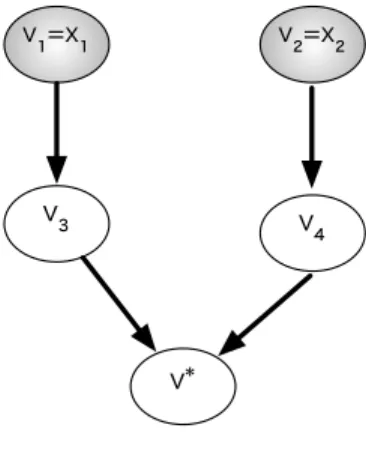
First, let us describe the proposed global feature expansion method using the ClassiNet shown in Figure6. Here, we
consider expanding an instancex=(x1,x2)⊤with two non-zero featuresv1=x1andv2=x2(x1,0, andx2,0). We
would like to compute the likelihoodp(v∗|x)of a vertexv∗as an expansion candidate for the instancex. From Figure6
we see that there are two possible paths reachingv∗starting from the original featuresx1andx2. Assuming that the
two paths are independent, we computep(v∗|x)as follows: p(v∗|x)=p(x 1)p(v3|x1)p(v ∗|v 3)+p(x2)p(v4|x2)p(v ∗|v 4) (12)
729 730 731 732 733 734 735 736 737 738 739 740 741 742 743 744 745 746 747 748 749 750 751 752 753 754 755 756 757 758 759 760 761 762 763 764 765 766 767 768 769 770 771 772 773 774 775 776 777 778 779 780 v₁=x₁ v₂=x₂ v₃ v₄ v*
Fig. 1. Computing the feature value of an expansion featurev∗for an instance that hasv1=x1andv2=x2as non-zero features.
The computation described in Figure6can be generalized for an arbitrary ClassiNetG(V,E,W), and an instance
x=(x1, . . . ,xd)⊤. For this purpose, let us define the set of non-cyclic paths connecting two verticesvi,vjinGto be
Γ(vi,vj). For the example shown in Figure6we have the two pathsx1→v3→v
∗
, andx2→v4→v
∗
. We compute
the likelihoodp(v∗|x)of a vertexv∗∈ Vbeing an expansion candidate ofxas follows: p(v∗|x)= d X k=1 * . , xkp(xk=vk) Y (a,b)∈Γ(xk,v∗) p(b|a)+ / -(13)
If a featurexk=0, then the likelihoods corresponding to paths starting fromxkwill be ignored in the computation of (13). The prior probabilities of featuresp(x
k)can be estimated from train data by dividing the number of instances that containxkby the total number of instances. Alternatively, we could set a uniform prior forp(xk)thereby considering all the words that occur in an instance equally. We follow the latter approach in our experiments.
The sum-product computation over paths can be efficiently computed by observing that it can be modeled as a label
propagation problem over a directed weighted graph, where an instancexis the initial state vector and the transition probabilities are given by the weight matrixW. Vertices that can be reached afterqhops are given byPq
i=1W
ix. Neighbours that are distantly located in the ClassiNet are less reliable as expansion candidates. To reduce the noise due
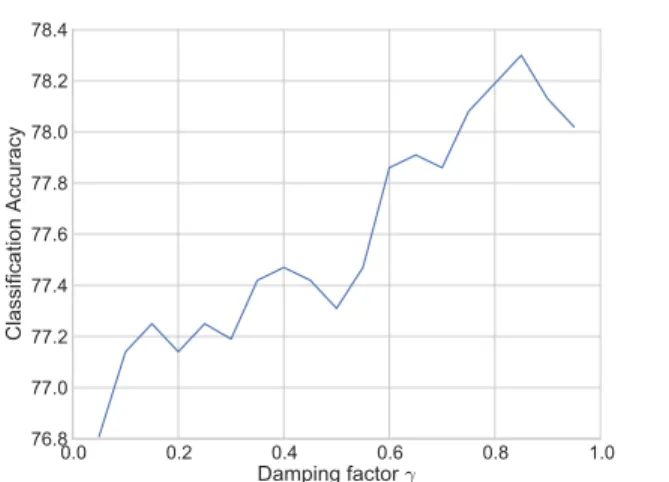
to distant (and potentially irrelevant) vertices during the propagation, we introduce a damping factor 0<γ ≤1 in the summation,Pq
i=1γ
iWix. In Section6.4, we experimentally study the effect of the level of damping on the classification accuracy of short-text classification.
The feature expansion methods we described above are used to predict missing features for both train and test
instances. We expand feature vectors representing the train/test instances, and assign unique identifiers to the expansion
features, thereby distinguishing between the original features and the expanded features. For example, given the positive
sentiment labeled train sentence “I love dogs”, we can represent it using the feature vector, [(I, 1), (love, 1), (dog, 1)]. Here, we assume that lemmatization has been conducted on the input and the featuredogshas been converted to its singular formdog. Let us further assume that from the trained ClassiNet we were able to predict thatcatis a related feature for dog, and the candidate scorep(cat|doд)=0.8. Next, we add the feature (EXP=cat, 0.8) to the feature vector representing this train instance, where the prefixEXP=indicates that it is a feature introduced by the expansion method and not a feature that existed in the original train instance. Distinguishing original vs. expansion features is useful when we
781 782 783 784 785 786 787 788 789 790 791 792 793 794 795 796 797 798 799 800 801 802 803 804 805 806 807 808 809 810 811 812 813 814 815 816 817 818 819 820 821 822 823 824 825 826 827 828 829 830 831 832
would like to learn different weights for the same feature depending on whether it is expanded or not. For example, if
a particular feature is not very useful as an expansion feature, it will be assigned a lower weight thereby effectively
pruning that feature out from the model learnt by the classifier.
The first step of learning a ClassiNet is learning the feature predictors. In this regard, any word embedding learning
method can be used for the purpose of learning feature predictors. Once the feature predictors are learnt, we can create
a ClassiNet in the same manner as we propose in this paper and use the ClassiNet created to perform feature expansion
using local/global feature expansion methods we propose in the paper. This view of ClassiNets illustrates the general
applicability of the proposed method.
5 A THEORETICAL ANALYSIS OF CLASSINETS
Before we empirically evaluate the performance of the proposed ClassiNets for feature expansion in short-text
classi-fication, let us analyze some interesting properties of ClassiNets. To simplify the analysis, let us assume that we are
using a ClassiNet for learning a linear classifierϕ∈Rdfor a binary classification task. Specifically, let us assume that we are given a train dataset{(x(k),y(k))}N
k=1
consisting ofNinstances, where each train instancekis represented by a feature vectorx(k)∈Rd. The binary target label assigned to thek-th train instance is denoted byy(k)∈ {1,−1}. For correctly classified train instancesx(k)we have,y(k)ϕ⊤x(k)>0.
We use the trained linear classifierϕ, and predict the label ˆyof an unseen test instance ˆxas follows:
ˆ y= 1 ifϕ⊤xˆ>0 −1 otherwise (14)
Let us assume that we have learnt a feature predictorhi that predicts whether thei-th feature exists in a given instance. As described in Section3.1, we can use any classification algorithm to learn the feature predictors. However,
as a concrete case, let us consider linear classifiers in this analysis. In the case of linear classifiers, we can represent the
feature predictor learnt for thei-th feature by the vectorµi. Following the notation introduced in Section3.1, we can write the feature predictorhi as follows:
hi(x)= 1 ifµi⊤x >0 −1 otherwise (15)
In the ClassiNets described in the paper so far, we used the predicted discrete labels as the values of the predicted
features during feature expansion. However, in this analysis let us consider the more general case where we use the
actual prediction score,µi⊤xas the contribution of the feature expansion towards thei-th feature.
We can construct the expanded feature vector,x∗∈Rd, of the feature vectorx∈Rdconsidering the inner-product betweenxand each of the feature predictorsµi as in (16).
x∗=
[(x1+µi
⊤x), . . . ,(x
i+µi⊤x), . . . ,(xd+µd⊤x)]⊤ (16)
Here, we denote thei-th dimension of the feature vectorxbyxi. We can transform the given train dataset{(x(k),y(k))}N k=1
by expanding each feature vector separately using (16), and use the expanded feature vectors to train a binary linear
classifierϕ∗. Following (14), we can useϕ∗to predict the label for a test instancex∗based on the prediction score given
833 834 835 836 837 838 839 840 841 842 843 844 845 846 847 848 849 850 851 852 853 854 855 856 857 858 859 860 861 862 863 864 865 866 867 868 869 870 871 872 873 874 875 876 877 878 879 880 881 882 883 884 by ϕ∗⊤x∗ = d X i=1 ϕ∗ i xi+µi⊤x = d X i=1 ϕ∗ ixi+ d X i=1 ϕ∗ iµi ⊤x = ϕ∗⊤x+ϕ∗⊤ Lx (17) = ϕ∗⊤( I+L)x (18)
Here,I∈Rd×dis a unit matrix, andL∈Rd×dis the matrix formed by arranging the feature predictorsµiin rows. In other words,L=[µ1. . .µd]⊤.
The first term in (17) corresponds to classifying the non-expanded (original) instancexusing the classifier trained using the expanded train dataset. The second term in (17) represents the prediction score due to feature expansion.
From (18) we see that performing feature expansion on a feature vectorxis equivalent to multiplying the matrix(I+L) intox. Therefore, local feature expansion methods described in Section4.1can be seen as projecting the train feature vectors into the samed-dimensional feature space spanned by the features that exist in the train instances. As a special case, we see that when we do not learn feature predictors we haveL=0, for which (17) reduces to the prediction score
ϕ∗⊤xof the binary linear classifier trained using non-expanded train instances.
5.1 Edge weights of ClassiNets
Recall that,wi jthe weight of the edge connecting the vertexito vertexjin a ClassiNet was defined by (1). In the case of binary linear feature predictorsµiandµjwe considered in the previous section, let us estimate the value ofwi j. Using the indicator function1defined by (10), we computeM11and(M11+M10)in (1) as follows:
M11= N X k=1 1[(y(k)x(k)⊤µi>0)∧(y(k)x(k)⊤µj>0)] (19) M11+M10= N X k=1 1[(y(k)x(k)⊤µi >0)] (20)
Let us assume that we sample instancesxfrom the train dataset randomly according to the distributionp(x). Then the expected counts inMˆ11andMˆ10in (19) and (20) can be expressed using the expected number of the correct classifications made by the feature predictorsµiandµj as follows:
ˆ M11=Ep(x) f 1[(yx⊤µi >0)∧(yx⊤µj>0)] g (21) ˆ M11+M10ˆ = Ep(x)f1[(yx⊤µi >0)] g (22)
Using the expected counts given by (21) and (22) we can compute the approximate value of the edge weightwi jˆ as follows: ˆ wi j= Ep(x) f 1[(yx⊤µi >0)∧(yx⊤µj >0)] g Ep(x)[1[(yx⊤µi >0)]] (23)
If we have a sufficiently large train dataset, then (23) provides an alternative procedure for estimating the edge
weights. We could randomly select samples from the train dataset, predict the featuresiandjfor those samples, and compute the expectations as ratio counts. We can repeat this procedure many times to obtain better approximations for
the edge weights. Although this is a theoretically feasible procedure for approximately computing the edge weights, it
885 886 887 888 889 890 891 892 893 894 895 896 897 898 899 900 901 902 903 904 905 906 907 908 909 910 911 912 913 914 915 916 917 918 919 920 921 922 923 924 925 926 927 928 929 930 931 932 933 934 935 936
can be slow in practice and might require many samples before we obtain a reliable approximation for the edge weights.
Therefore, the edge weight computation method described in Section3.3is more appropriate for practical purposes.
5.2 Analysis of the Global Feature Expansion Method
We already showed in (18) that local feature expansion methods can be considered as feature vector transformation
methods by a matrix(I+L). However, an important strength of ClassiNet is that we can propagate the predicted features over the network using the global feature expansion method described in Section4.2.
Let us denote the edge-weight matrix of the ClassiNetGbyW. The(i,j)-th element ofWis denoted bywi j. The connection between edge weightswi j and the feature predictorsµi andµj is given by (23). In the global feature expansion method, we repeatedly propagate the predicted features across the network, which can be seen as a repeated
multiplication usingγW, whereγ is the damping factor described in Section4.2. Observing this connection, we can derive the prediction score under the global feature expansion method similar to (18) as follows:
ϕ∗⊤x∗ = ϕ∗⊤ I+γW+. . .+γqWqx = ϕ∗⊤(I−γW)−1( I−γ(q+1) W(q+1))x (24)
For the summation shown in (24) to hold, and the matrix(I−γW)to be invertible, for all eigenvaluesλr ofWwe requireγ|λr|<1. This requirement can be met in practice by a sufficiently small damping factor. For example, we could setγ =1/(1+|λmax||), where|λmax|is the eigenvalue ofWwith the maximum absolute value.
As a special case where we propagate the features without truncating, we haveq→ ∞, for which we obtain the prediction score given in (25).
ϕ∗⊤x∗=ϕ∗⊤(
I−γW)−1
x (25)
From (25), we see that, similar to the local feature expansion methods, the global feature expansion method can also be
seen as projecting the input feature vectorxusing the matrix(I−γW)−1.
6 EXPERIMENTS
We create a ClassiNet using 257,306 unlabeled sentences from the Large Movie Review dataset1. Each word in this dataset
is uniquely represented by a vertex in the ClassiNet. We learn linear predictor for each feature using automatically
selected positive (reviews where the target feature appears) and negative (reviews where the target feature does not
appear) training instances. The ClassiNet created from this dataset contains 489,000 vertices. This ClassiNet is used in all the experiments described in the remainder of this paper.
For evaluation purposes we use four binary classification datasets: the Stanford sentiment treebank (TR)2(903 positive test instances and 903 negative test instances), movie reviews dataset (MR) [Pang and Lee 2005] (5331 positive instances and 5331 negative instances), customer reviews dataset (CR) [Hu and Liu 2004] (925 positive instances and 569 negative instances), and subjectivity dataset (SUBJ) [Pang and Lee 2004] (5000 positive instances and 5000 negative instances). We perform five-fold cross-validation in all datasets, except in the Stanford sentiment treebank where there
exists a pre-defined test and train split. In each dataset, we use the train portion to learn a binary classifier. Next, we use
the trained ClassiNet to expand the feature vectors for the test instances. We then measure the classification accuracy
1
http://ai.stanford.edu/~amaas/data/sentiment/
2
http://nlp.stanford.edu/sentiment/treebank.html